Decomposed Iterative Optimal Power Flow with Automatic Regionalization


Abstract
1. Introduction
- (i)
- Optimality: the OPF is non-convex in both its objective function and constraints, and hence finding the global optimum is not guaranteed.
- (ii)
- Scalability: OPF is an NP-hard problem and the complexity usually grows exponentially with the size of the system. It is quite possible that a proposed solution works well for small systems, but fails to converge to a solution for large systems.
- (i)
- The decomposition is achieved manually in an ad hoc manner without any guidance. To date, there has been no reported effort to utilize the topology and property of the original system to conduct better regionalization such that the distributed OPF can achieve improved computational efficiency and optimality.
- (ii)
- Limited interactions among subsystems are involved during the optimization process. The obtained solutions are ad hoc combinations of the optimal solutions for local subsystems, which compromise the optimality for the whole system.
- (iii)
- Only one decomposition is studied, which means that the optimization is made for the decomposed local parts without a global consideration of the entire system.
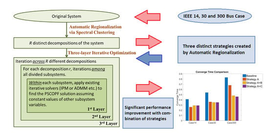
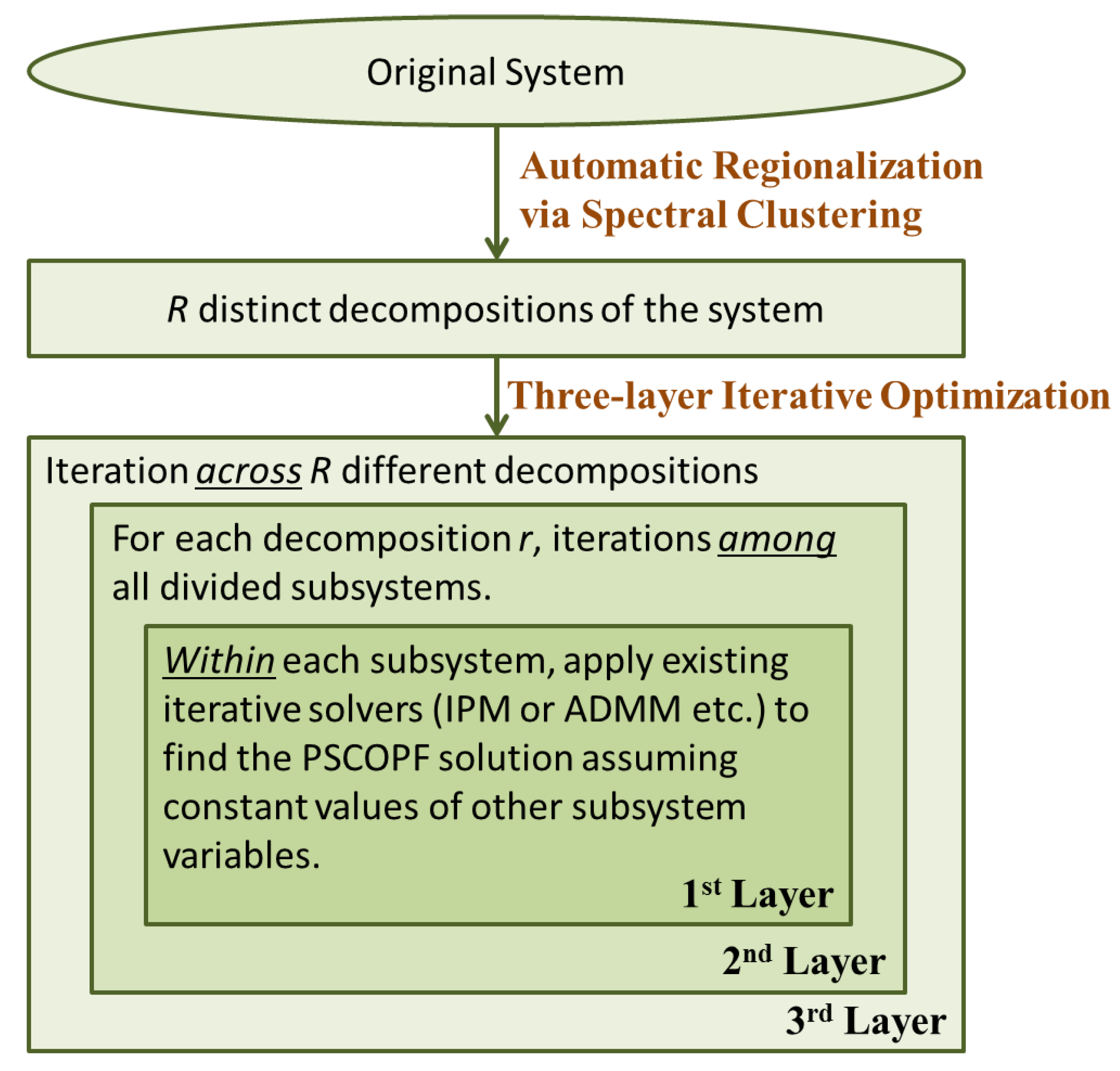
- Automatic: an automatic regionalization technique is proposed to decompose the original large system into smaller subsystems, which will balance the computational loads of the resultant subsystems and achieve the maximum independence of the variables in different subsystems to accelerate the convergence speed in iterative optimization.
- General: at the first level, many existing OPF problems or general optimization tools can be applied. We first adopt the two most popular OPF tools, one based on the interior-point method (IPM) and the other based upon ADMM.
- Global: the proposed three-layer framework, especially the added third layer of iteration among different decompositions, will greatly increase the extensiveness of the dimensions the algorithm searches and make the optimization results global in view.
2. Problem Statement
2.1. Standard OPF Formulation
2.2. Decomposed OPF Formulation
3. Automatic Regionalization Based OPF (AR-OPF)
3.1. Overview of the Algorithm
3.2. Automatic Regionalization via Spectral Clustering
- (1)
- Topology Based Similarity (TBS): The simplest method is utilizing the topology of the system directly to define the similarity which results in creating a weighted adjacency matrix with 1 s representing a transmission line connects the buses and 0s for otherwise.
- (2)
- Measurement-Based Similarity (MBS): The states of a bus can only affect its neighbors during operation, which means that there is an available measurement that both buses are involved simultaneously. More specifically, the similarity considers whether there is at least one power flow measurement available on a transmission line, or one power injection measurement available at either one of the buses connected to the line.
- (3)
- Weighted Measurement-Based Similarity (WMBS): In fact, no two of the buses have the same amount of measurements involved, and not all measurements have the same amount of effect in coupling those involved buses. Under certain circumstances, it will be more favorable to cluster two strongly coupled buses into one region and divide two weakly coupled buses into different regions. Therefore WMBS is considering not only the availability of the measurements, but also the amount and impact of the measurements.
3.3. Cross-Subsystem Variable Update
3.3.1. Subsystem Variable Update
| Algorithm 1: Decomposed OPF. |
| 1 Initialization: Set and initialize and |
| 2 Private variable update: Set and . Each bus updates locally, where we let be the primal and dual (possibly) optimal variables achieved for the following problem: |
| 3 Net variable update: We denote as the solution to the problem minimize |
| 4 Dual variable update: Each bus updates its dual variable as |
| 5 Stopping criterion check: set . If the stopping criterion is not reached, go to step 2, otherwise stop and return . |
3.3.2. Cross-Subsystem
4. Simulation and Results
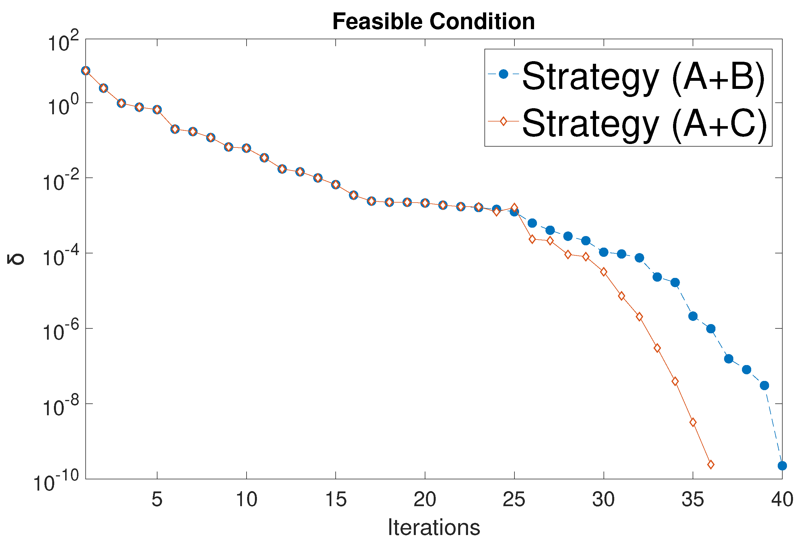
4.1. Simulation Result Analysis
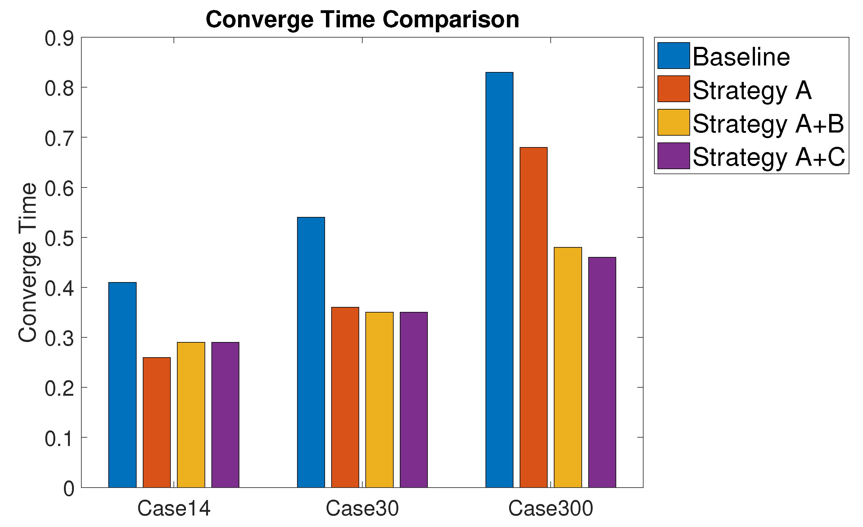
4.2. Time Efficiency and Scalability
5. Conclusions
Author Contributions
Funding
Acknowledgments
Conflicts of Interest
References
- Carpentier, J. Contribution a l’etude du dispatching economique. Bull. De La Soc. Fr. Des Electr. 1962, 3, 431–447. [Google Scholar]
- Frank Stephen, S.I.; Steffen, R. Optimal power flow: A bibliographic survey I. Energy Syst. 2012, 221–258. [Google Scholar] [CrossRef]
- Frank, S.; Steponavice, I.; Rebennack, S. Optimal power flow: A bibliographic survey II. Energy Syst. 2012, 259–289. [Google Scholar] [CrossRef]
- Wang, Y.; Bai, X.; Wei, H.; Fujisawa, K. Semidefinite programming for optimal power flow problems. Int. J. Electr. Power Energy Syst. 2008, 30, 383–392. [Google Scholar]
- Cavoukian, A.; Polonetsky, J.; Wolf, C. Smartprivacy for the smart grid: Embedding privacy into the design of electricity conservation. Identity Inf. Soc. 2010, 3, 275–294. [Google Scholar] [CrossRef]
- Andersen, M.S.; Hansson, A.; Vandenberghe, L. Reduced-Complexity Semidefinite Relaxations of Optimal Power Flow Problems. IEEE Trans. Power Syst. 2014, 29, 1855–1863. [Google Scholar] [CrossRef]
- Madani, R.; Ashraphijuo, M.; Lavaei, J. Promises of Conic Relaxation for Contingency-Constrained Optimal Power Flow Problem. IEEE Trans. Power Syst. 2016, 31, 1297–1307. [Google Scholar] [CrossRef]
- Kocuk, B.; Dey, S.S.; Sun, X.A. Inexactness of SDP Relaxation and Valid Inequalities for Optimal Power Flow. IEEE Trans. Power Syst. 2016, 31, 642–651. [Google Scholar] [CrossRef]
- Huang, S.; Wu, Q.; Wang, J.; Zhao, H. A Sufficient Condition on Convex Relaxation of AC Optimal Power Flow in Distribution Networks. IEEE Trans. Power Syst. 2017, 32, 1359–1368. [Google Scholar] [CrossRef]
- Coffrin, C.; Hijazi, H.L.; Hentenryck, P.V. Strengthening the SDP Relaxation of AC Power Flows With Convex Envelopes, Bound Tightening, and Valid Inequalities. IEEE Trans. Power Syst. 2017, 32, 3549–3558. [Google Scholar] [CrossRef]
- Kocuk, B.; Dey, S.S.; Sun, X.A. New Formulation and Strong MISOCP Relaxations for AC Optimal Transmission Switching Problem. IEEE Trans. Power Syst. 2017, 32, 4161–4170. [Google Scholar] [CrossRef]
- Bahrami, S.; Therrien, F.; Wong, V.W.S.; Jatskevich, J. Semidefinite Relaxation of Optimal Power Flow for AC DC Grids. IEEE Trans. Power Syst. 2017, 32, 289–304. [Google Scholar] [CrossRef]
- Lorca, A.; Sun, X.A. The Adaptive Robust Multi-Period Alternating Current Optimal Power Flow Problem. IEEE Trans. Power Syst. 2018, 33, 1993–2003. [Google Scholar] [CrossRef]
- Venzke, A.; Halilbasic, L.; Markovic, U.; Hug, G.; Chatzivasileiadis, S. Convex Relaxations of Chance Constrained AC Optimal Power Flow. IEEE Trans. Power Syst. 2018, 33, 2829–2841. [Google Scholar] [CrossRef]
- Baldick, R.; Kim, B.H.; Chase, C.; Luo, Y. A fast distributed implementation of optimal power flow. IEEE Trans. Power Syst. 1999, 14, 858–864. [Google Scholar] [CrossRef]
- Kim, B.H.; Baldick, R. A comparison of distributed optimal power flow algorithms. IEEE Trans. Power Syst. 2000, 15, 599–604. [Google Scholar] [CrossRef]
- Nogales, F.J.; Prieto, F.J.; Conejo, A.J. A Decomposition Methodology Applied to the Multi-Area Optimal Power Flow Problem. Ann. Oper. Res. 2003, 99–116. [Google Scholar] [CrossRef]
- Lam, A.Y.S.; Zhang, B.; Tse, D.N. Distributed algorithms for optimal power flow problem. In Proceedings of the 2012 IEEE 51st IEEE Conference on Decision and Control (CDC), Maui, HI, USA, 10–13 December 2012; pp. 430–437. [Google Scholar]
- Erseghe, T. Distributed Optimal Power Flow Using ADMM. IEEE Trans. Power Syst. 2014, 29, 2370–2380. [Google Scholar] [CrossRef]
- Magnson, S.; Weeraddana, P.C.; Fischione, C. A Distributed Approach for the Optimal Power-Flow Problem Based on ADMM and Sequential Convex Approximations. IEEE Trans. Control Netw. Syst. 2015, 2, 238–253. [Google Scholar] [CrossRef]
- Carpentier, J. Optimal power flows. Int. J. Electr. Power Energy Syst. 1979, 1, 3–15. [Google Scholar] [CrossRef]
- Wang, D.; Yang, L.; Florita, A.; Alam, S.M.S.; Elgindy, T.; Hodge, B. Automatic regionalization algorithm for distributed state estimation in power systems. In Proceedings of the 2016 IEEE Global Conference on Signal and Information Processing (GlobalSIP), Washington, DC, USA, 7–9 December 2016; pp. 787–790. [Google Scholar]
- Shi, J.; Malik, J. Normalized Cuts and Image Segmentation. IEEE Trans. Pattern Anal. Mach. Intell. 2000, 22, 888–905. [Google Scholar]
- Wang, H.; Murillo-Sanchez, C.E.; Zimmerman, R.D.; Thomas, R.J. On Computational Issues of Market-Based Optimal Power Flow. IEEE Trans. Power Syst. 2007, 22, 1185–1193. [Google Scholar] [CrossRef]
- Zimmerman, R.D.; Murillo-Sanchez, C.E.; Thomas, R.J. MATPOWER: Steady-State Operations, Planning, and Analysis Tools for Power Systems Research and Education. IEEE Trans. Power Syst. 2011, 26, 12–19. [Google Scholar] [CrossRef]
- Zimmerman, R.D.; Murillo-Sanchez, C.E. MATPOWER. Version 7.0. Available online: https://matpower.org/dld/1244/ (accessed on 18 September 2020).
- Zimmerman, R.D.; Murillo-Sanchez, C.E. MATPOWER User’s Manual Version 7.0. Available online: https://matpower.org/docs/manual.pdf (accessed on 18 September 2020).
- The Mathworks, Inc. MATLAB Version 9.3.0.713579 (R2017b); The Mathworks, Inc.: Natick, MA, USA, 2017. [Google Scholar]
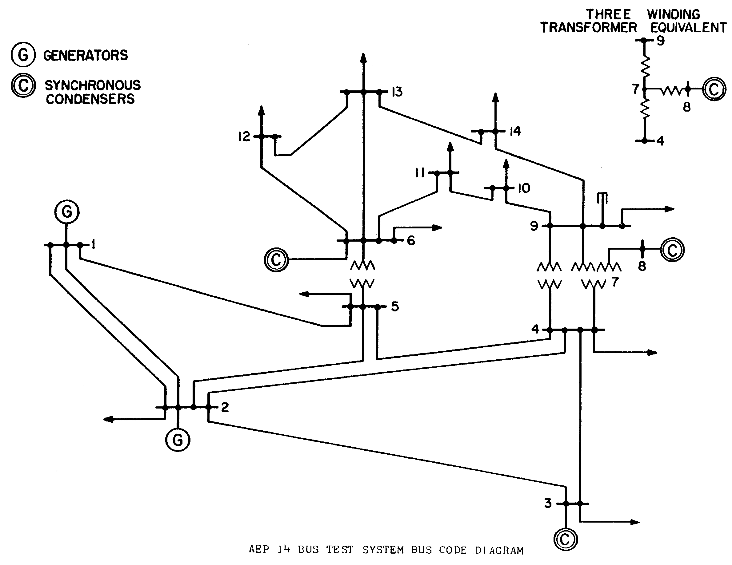
- Christie, R. 14 Bus Power Flow Test Case. Available online: http://labs.ece.uw.edu/pstca/pf14/pg_tca14bus.htm (accessed on 15 September 2020).


| Regionalization | Region 1 | Region 2 | Region 3 | Region 4 |
|---|---|---|---|---|
| Manual Case 1 | 1, 2, 5 | 3, 4, 7, 8, 9 | 10, 11, 14 | 6, 12, 13 |
| Manual Case 2 | 1, 2, 5 | 3, 4, 7, 8 | 9, 10, 14 | 6, 11, 12, 13 |
| TBS-AR (A) | 1, 2, 3, 4, 5 | 7, 8, 9 | 10, 11 | 6, 12, 13, 14 |
| MBS-AR (B) | 1, 2,3,5 | 4, 7, 8, 9 | 10, 11 | 6, 12, 13, 14 |
| WMBS-AR (C) | 1, 2, 3, 5 | 4, 7, 8, 9, 14 | 10, 11 | 6, 12, 13 |
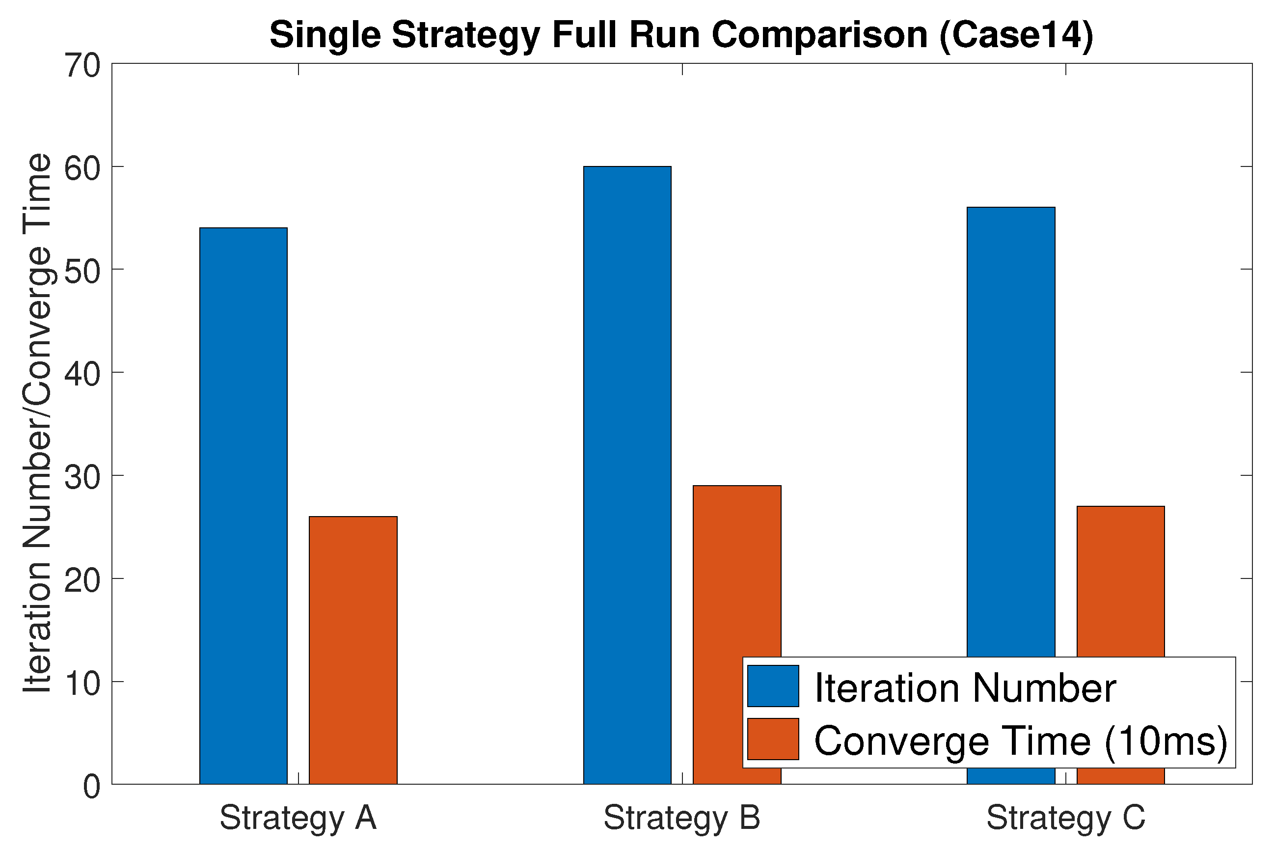
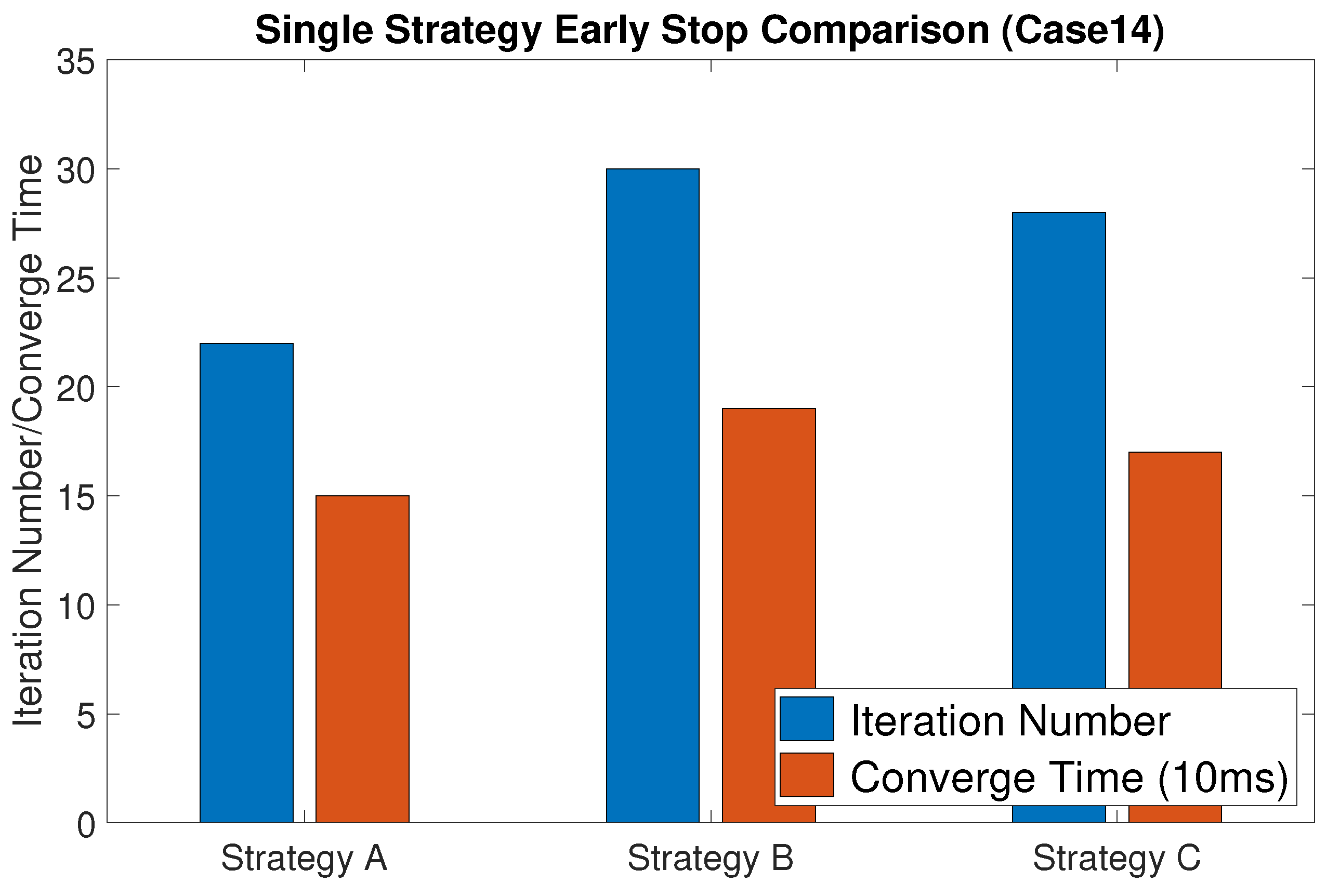
| Results | Original | Strategy A | Strategy B | Strategy C |
|---|---|---|---|---|
| Converge Time (s) | 0.41 | 0.26 | 0.29 | 0.27 |
| Iteration numbers | 12 | 54 | 60 | 56 |
| Objfcn Value ($/h) | 8081.53 | 8081.53 | 8081.53 | 8081.53 |
| Total Gen P (MW) | 268.29 | 268.29 | 268.29 | 268.29 |
| Total Gen Q (MVar) | 67.63 | 67.63 | 67.63 | 67.63 |
| Branch Loss P (MW) | 9.287 | 9.287 | 9.287 | 9.287 |
| Branch Loss Q (MVar) | 39.16 | 39.16 | 39.16 | 39.16 |
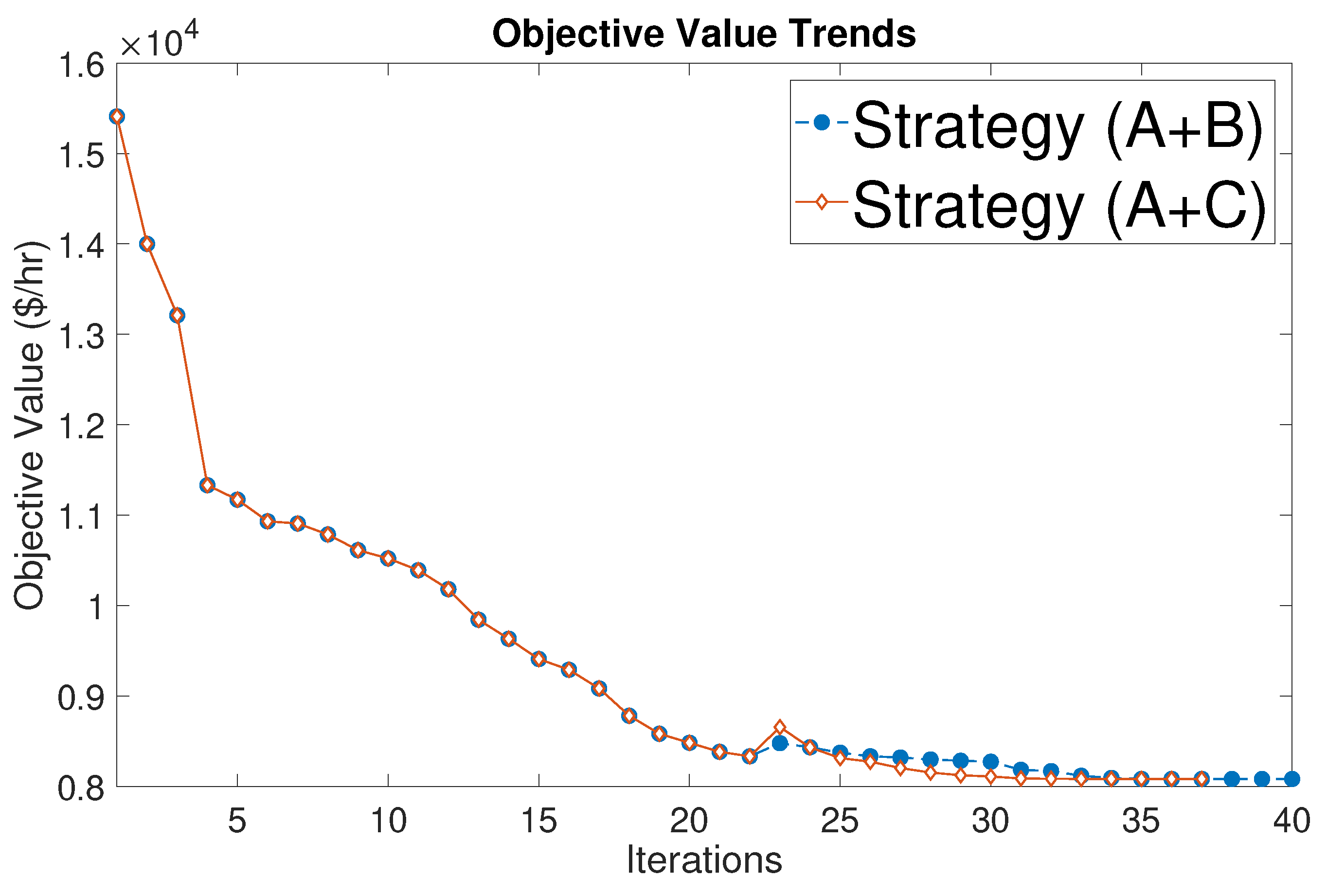
| Results | Original | AROPF (A+B) | AROPF (A+C) |
|---|---|---|---|
| Converge Time (s) | 0.41 | 0.29 | 0.29 |
| Iteration numbers | 12 | 40 (22+18) | 36 (22+14) |
| Objfcn Value ($/h) | 8081.53 | 8081.53 | 8081.53 |
| Total Gen P (MW) | 268.29 | 268.29 | 268.29 |
| Total Gen Q (MVar) | 67.63 | 67.63 | 67.63 |
| Branch Loss P (MW) | 9.287 | 9.287 | 9.287 |
| Branch Loss Q (MVar) | 39.16 | 39.16 | 39.16 |
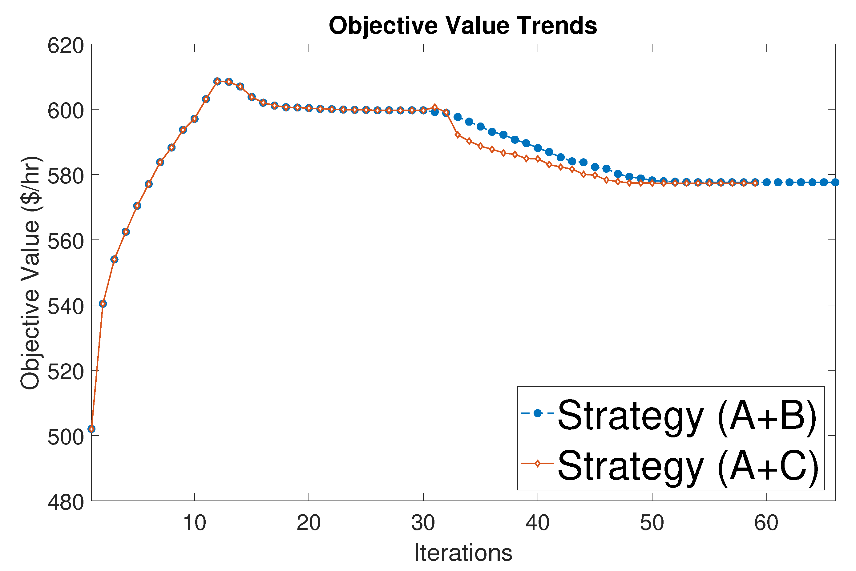
| Results | Original | AROPF (A+B) | AROPF (A+C) |
|---|---|---|---|
| Converge Time (s) | 0.54 | 0.35 | 0.35 |
| Iteration numbers | 15 | 66 (33+33) | 59 (33+26) |
| Objfcn Value ($/h) | 576.89 | 577.63 | 577.39 |
| Total Gen P (MW) | 192.06 | 192.81 | 192.34 |
| Total Gen Q (MVar) | 105.08 | 106.58 | 106.21 |
| Branch Loss P (MW) | 2.860 | 2.772 | 2.825 |
| Branch Loss Q (MVar) | 13.33 | 12.66 | 12.75 |
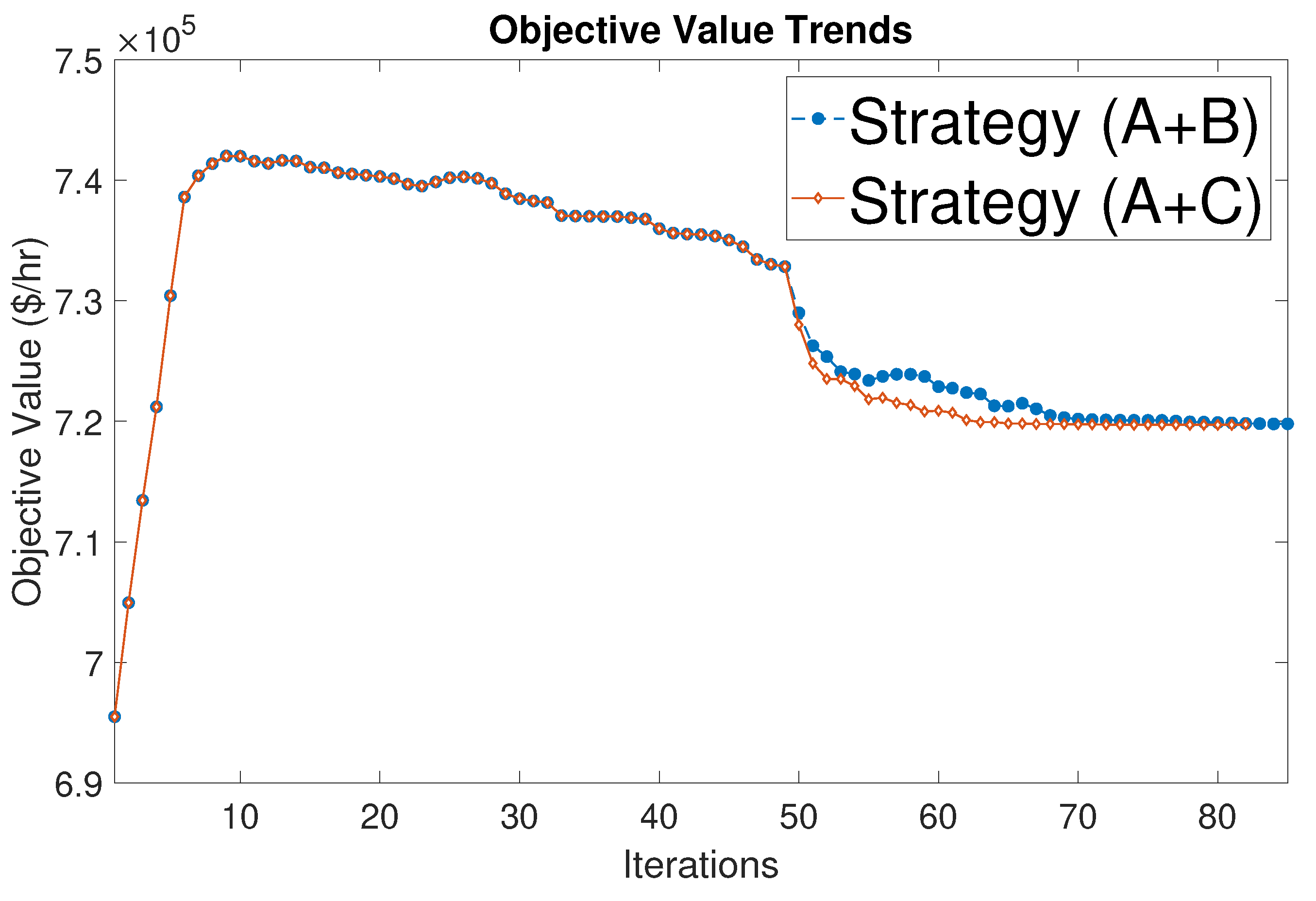
| Results | Original | AROPF (A+B) | AROPF (A+C) |
|---|---|---|---|
| Converge Time (s) | 0.83 | 0.48 | 0.46 |
| Iteration numbers | 19 | 85 (49+36) | 82 (49+33) |
| Objfcn Value ($/h) | 719,725.11 | 719,790.85 | 719,727.16 |
| Total Gen P (MW) | 32,678.4 | 32,682.1 | 32,680.7 |
| Total Gen Q (MVar) | −9240.1 to 14,090.2 | −9239.7 to 14,093.1 | −9239.9 to 14,091.2 |
| Branch Loss P (MW) | 302.78 | 303.16 | 302.88 |
| Branch Loss Q (MVar) | 4599.97 | 4600.89 | 4600.11 |
© 2020 by the authors. Licensee MDPI, Basel, Switzerland. This article is an open access article distributed under the terms and conditions of the Creative Commons Attribution (CC BY) license (http://creativecommons.org/licenses/by/4.0/).
Share and Cite
Zheng, X.; Duan, D.; Yang, L.; Wang, H. Decomposed Iterative Optimal Power Flow with Automatic Regionalization. Energies 2020, 13, 4987. https://doi.org/10.3390/en13184987
Zheng X, Duan D, Yang L, Wang H. Decomposed Iterative Optimal Power Flow with Automatic Regionalization. Energies. 2020; 13(18):4987. https://doi.org/10.3390/en13184987
Chicago/Turabian StyleZheng, Xinhu, Dongliang Duan, Liuqing Yang, and Haonan Wang. 2020. "Decomposed Iterative Optimal Power Flow with Automatic Regionalization" Energies 13, no. 18: 4987. https://doi.org/10.3390/en13184987
APA StyleZheng, X., Duan, D., Yang, L., & Wang, H. (2020). Decomposed Iterative Optimal Power Flow with Automatic Regionalization. Energies, 13(18), 4987. https://doi.org/10.3390/en13184987