Article

Recognition of Variable-Speed Equipment in an Air-Conditioning System Using Numerical Analysis of Energy-Consumption Data

1
Department of Building Science, Tsinghua University, Beijing 100084, China
2
School of Mechanical Engineering, Southwest Jiaotong University, Chengdu 610031, China
3
State Key Laboratory of Air-conditioning Equipment and System Energy Conservation, Zhuhai 519070, China
4
Gree Electric Appliances, Inc. of Zhuhai, Zhuhai 519070, China
*
Author to whom correspondence should be addressed.
Energies 2020, 13(18), 4975; https://doi.org/10.3390/en13184975
Submission received: 30 July 2020 / Revised: 13 September 2020 / Accepted: 18 September 2020 / Published: 22 September 2020
(This article belongs to the Special Issue Data-Driven Energy-Cost Analysis of HVAC System for Buildings)

Abstract

:
Motor-driven equipment (ME) is one of the key components in an air-conditioning system, which contributes to the vast majority of the total energy consumption by air-conditioning systems. Distinguishing variable- and constant-speed equipment is important since the energy simulation models of the two types differ. Traditionally, types of ME are known in advance, and energy consumption data are consequently analyzed. However, in the application scenarios of energy consumption data mining, precedent information on the ME type could be missing. Thus, this study applies this process in reverse, providing new insight into energy consumption data of ME to recognize variable-speed ME in an air-conditioning system. The energy consumption data of ME in an air-conditioning system implemented in a commercial building were collected and numerically analyzed. A proposed simple parameter, coefficient of the median, and several numerical parameters were calculated and used to distinguish variable- from constant-speed ME. Results showed that the energy consumption data distributions of the two types of ME differed. The proposed coefficient of the median could successfully distinguish variable- from constant-speed ME, and it could be applied as an important step in energy consumption data mining of air-conditioning systems.

Graphical Abstract

1. Introduction

Air-conditioning systems are major sources of energy consumption in buildings [1,2]. Therefore, energy conservation for air-conditioning systems is of primary importance in building energy saving. In an air-conditioning system, the operation of various types of equipment is driven by motors, such as electric chillers, fans, and pumps. Therefore, motor-driven equipment (ME) is a key component in air-conditioning systems, especially in fluid transport subsystems. These subsystems transport refrigerant, cooled/heated air, chilled water, condensing water, or even a glycol solution to ensure the working cycle of the system. The energy consumed by ME makes up the vast majority of the total energy consumption of air-conditioning systems [3]. Thus, reducing the energy costs of ME may be an important approach to energy conservation for air-conditioning systems. Variable-speed ME has been used in air-conditioning systems for more than 40 years [4]. By changing the working frequency corresponding to flow-rate variations, variable-speed ME can generally cost less energy than constant-speed ME under the same conditions [5,6,7].
For air-conditioning systems equipped with both variable- and constant-speed ME, recognition of each equipment type is vital for energy-consumption analysis, particularly for energy simulations of ME, since the models of variable- and constant-speed ME are different [8,9,10]. In previous studies, the type of ME was known in advance, and the energy consumption data of the ME were then analyzed on the basis of known conditions [11,12,13]. For instance, several studies focused on the significant benefits brought about by the application of variable-speed drive technology to various types of ME of air-conditioning systems. For example, studies achieved comparative analyses of the energy performance of variable-speed compressors [4,14], pumps [15,16,17], fans [18,19], chiller plants [20,21,22], and even entire systems [23,24] against the performance of on/off-controlled constant-speed ME. However, what about going in reverse?
Normally, variable/constant-speed ME of an air-conditioning system is clarified by the designer during its design process. However, with the development of information technology and easy access to operating data, data-mining research through the use of actual operating data is now an important and effective tool for energy-saving diagnosis and operational optimization for air-conditioning systems [25]. In the context of automatic data mining of massive energy consumption data for energy-saving diagnosis [26,27,28], the codes normally have no such precedent information [29]. Instead, all the information is expected to come from the data-mining analysis of actual energy consumption data. It is, therefore, of great interest to investigate whether the energy consumption data of ME can reveal the characteristics and thus determine the type of ME. In addition, if the type of ME is already known, such an investigation could also check whether the variable-speed ME is working properly. Studies previously demonstrated the feasibility of using the intrinsic correlations of operational data to infer the operating state of air-conditioning systems [30]. However, more studies focused on the diagnosis of system faults using different methods, such as neural networks [31,32], wavelet analysis [33,34], principal component analysis [35,36], and combinatorial methods [37,38], or on making predictions related to future data by using existing data [39,40]. The few analyses of variable-speed systems were also based on the premise that it is known in advance whether it is a variable-speed device or not [41,42]. The paucity of literature examining the above issue prompted us to carry out this study.
This study aims to provide new insights into energy consumption data of ME, applied to the recognition of variable-speed ME in an air-conditioning system. The energy-consumption data of ME in an air-conditioning system operating in a commercial building were collected and numerically analyzed. A simple indicator parameter proposed by the study, coefficient of the median, and several numerical parameters were calculated and used to distinguish variable- from constant-speed ME. The results deepen our understanding of energy consumption characteristics related to the ME, and they provide insight into an important aspect of energy consumption-data mining in air-conditioning systems.

2. Methodology

2.1. ME in the Studied Air-Conditioning System

The studied air-conditioning system was installed in a five-story commercial building with an area of 30,000 m2 located in Shenzhen, China. The system was coupled with an ice-storage system in order to take advantage of the lower electricity price at night. As shown in Figure 1, the system included two constant-speed chillers (Ch-1 and Ch-2) of the same brand and model, five sets of variable-speed air-handling units (AHUs; AHU-1, AHU-2, AHU-3, AHU-4, and AHU-5) of the same brand but different models, and nine pumps of the same brand but different models. The chillers, AHUs, and pumps were each of different brands, all of which were newly set up in the same year and operated properly for three years up to the time of data collection for this study. Furthermore, the nine pumps included three condensing-water pumps (CWP-1, CWP-2, and CWP-3) to achieve a condensing-water circle between chiller and cooling tower, three chilled-water pumps (ChWP-1, ChWP-2, and ChWP-3) to guarantee a chilled-water loop between heat exchanger and air-handling units at the terminal, and three glycol water pumps (GWP-1, GWP-2, and GWP-3) to transport the glycol solution between any two or all three of the chiller, the ice-storage tank, and the heat exchanger. Four of the nine pumps could operate with variable speed, while the other five worked with constant speed. However, before this study, the authors were not aware of which pumps were variable-speed ME. This was later established on the basis of energy consumption data mining.

2.2. Collection and Processing of ME Energy Consumption Data

A comprehensive energy consumption monitoring platform was established for the air-conditioning system to monitor the electricity consumption of each component of the system. However, due to logistics and other constraints, the energy consumption of cooling towers was not available in the present case. Therefore, a follow-up study was employed to determine the energy consumption data of the remaining ME, including the aforementioned nine pumps, five AHUs, and two chillers. As it was expected that this study would be a true reflection of the use of the ME, data collection was conducted without any planned interventions or controls. For the involved ME, the electricity consumption of each device was recorded every hour from 19 May to 20 August 2013. Lastly, 2262 electricity consumption items were obtained for each device.
The raw data of electricity consumption of the ME and the corresponding time downloaded from the platform were then processed before numerical analysis. First, data with zero electricity consumption were eliminated since they demonstrated that the ME was turned off at the time. Second, data with duplicated time records were deleted to avoid repeated counts. Lastly, a processed electricity consumption data list with a time record was obtained for each device.

2.3. Numerical Analysis of Energy Consumption Data

Data distribution analysis can reveal the characteristics of energy consumption data. Nevertheless, using data distribution fitting can lead to extremely heavy computational loads, particularly with massive amounts of data. Instead, the numerical characteristics of data are important for data statistics, as they can intuitively reveal the data distribution and can easily be obtained. In this study, some commonly used parameters were introduced, including dimensional parameters such as maximal value Emax, minimal value Emin, range Erange, mean value Emean, median value Emedian, mode Emode, variance Evar, and standard deviation Esd, and dimensionless parameters, including coefficient of variation Cv, coefficient of skewness Cs, and coefficient of kurtosis Ck.
Specifically, coefficient of variation Cv is defined as the ratio of standard deviation to the mean value of data [43], calculated using Equation (1).
C v = E s d E m e a n .
Coefficient of skewness Cs indicates the asymmetry of data distribution [44], calculated using Equation (2).
C s = 1 n i = 1 n ( E i E m e a n ) 3 E v a r 3 / 2 ,
where n represents the data quantity, and Ei represents the electricity consumption of i.
Coefficient of kurtosis Ck reveals the existence of extreme values in the data list [45], calculated using Equation (3).
C k = 1 n i = 1 n ( E i E m e a n ) 4 E v a r 2 3 ,
where the parameters are the same as those in Equation (2).
Additionally, a simple dimensionless parameter, coefficient of the median Cm, is proposed in the present study, defined as the ratio of the difference between the maximum and median to the range, calculated using Equation (4). The theoretical and practical flow underlying the proposition of Cm is discussed in Section 4.2.
C m = E m a x E m e d i a n E r a n g e .
The parameters mentioned above were calculated or recorded to understand the numerical characteristics of energy consumption for each device. Afterward, the parameters were compared to determine if their disparities could be used to directly recognize the variable-speed ME.

3. Results

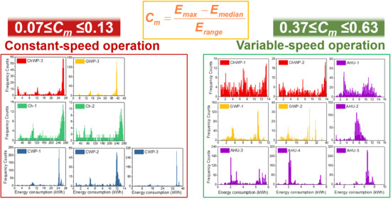
3.1. ME Energy Consumption Distributions

The energy consumption distributions of the 16 ME items are shown in Figure 2. Some obvious differences could be witnessed among the devices. Taking the nine pumps as an example, some of the pumps consumed as much as >40 kWh electricity, such as GWP-3, while some consumed much less electricity, e.g., ChWP-1 and CWP-2. From the perspective of distribution, for some pumps, such as ChWP-3 and CWP-3, most of the energy consumption data were grouped near the maximal value. The high-energy-consumption data appeared hundreds of times more often than low-energy-consumption data did. In comparison, for other pumps, such as ChWP-1 and ChWP-2, energy consumption data were distributed more uniformly, while for GWP-1 and GWP-2, several different peaks could be seen in the distribution. The differences in energy consumption distribution among the ME items may provide inspiration for the recognition of variable-speed equipment. More detailed information on numerical analysis can be found in Section 3.2.

3.2. Numerical Characteristics of Energy Consumption Data

The numerical parameters of the energy consumption data for each ME item were calculated, and they are listed in Table 1. As seen, most dimensional parameters of the AHUs were generally the lowest among all the ME, while the two chillers presented most of the highest dimensional parameters. Additionally, sorting the devices on the basis of these dimensional parameters resulted in individual differences. When referring to dimensionless parameters, the lowest Cs and Cv and the highest Ck were found for AHU-5, indicating that the energy consumption data were highly concentrated near the maximal value. In comparison, for ChWP-1, ChWP-2, GWP-1, GWP-2, AHU-1, and AHU-3, Cs and Cv were much higher, while Ck was much lower, implying more uniform distributions.

3.3. Recognition of Variable-Speed ME

3.3.1. Recognition of Variable-Speed Pumps

As seen in Table 1, the values of Cv and Cm allowed for dividing the pumps into two groups: one with comparatively high Cv and Cm, including ChWP-1, ChWP-2, GWP-1, and GWP-2, and another with comparatively low Cm and Cv, consisting of ChWP-3, CWP-1, CWP-2, CWP-3, and GWP-3. To highlight the two groups, a scatter matrix based on numerical parameters is shown in Figure 3.
Figure 3 clearly shows that the nine pumps were divided into two groups, as shown in row 9 and column 5. The four red points in the top-right corner represent ChWP-1, ChWP-2, GWP-1, and GWP-2. This high value indicated that the energy consumption data of the four pumps were not concentrated at the extrema but were distributed fairly uniformly, which was in accordance with the operation characteristics of variable-speed pumps. Therefore, it was assumed that ChWP-1, ChWP-2, GWP-1, and GWP-2 were variable-speed ME, while the five other pumps were constant-speed ME.
With the information transmitted from the field, the assumption was then validated, indicating the successful recognition of variable-speed pumps by this study.
Cm and Cs could be used to individually distinguish the two groups of pumps, as seen in row 4 combined with column 5 and row 9, respectively, while other numerical parameters failed. However, the calculation of Cm was much easier than that of Cs. Therefore, Cm may be a good parameter to be used as an indicator in the recognition of variable-speed pumps.

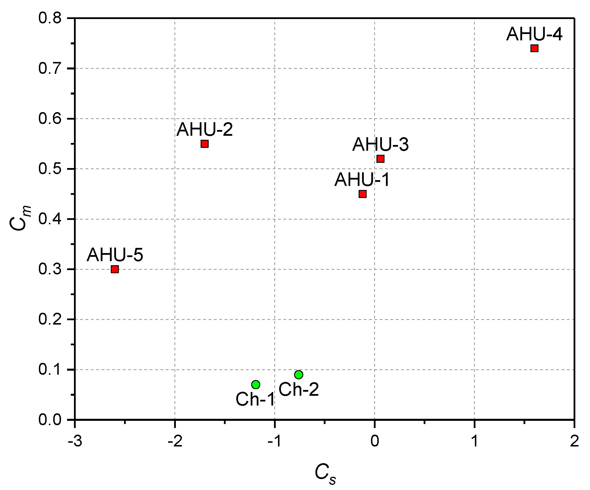
3.3.2. Verifiable Recognition of Variable-Speed AHUs and Constant-Speed Chillers

From the information transmitted on site, the five AHUs were operated with variable speed, while the two chillers worked with constant speed. Therefore, the recognition of AHUs and chillers could be further investigated to verify the applicability of the two indicators of Cm and Cs. The values of Cm and Cs of each of the seven devices are visually compared in Figure 4. Interestingly, Cm could be used to distinguish variable-speed AHUs and constant-speed chillers by using a single threshold (0.09–0.30), whereas Cs failed to facilitate recognition despite its applicability for pumps. The possible reason for this is discussed in Section 4.2.
The results presented thus far support the idea that proposed parameter Cm could be a good indicator in the recognition of variable-speed equipment.

4. Discussions

4.1. Feature Selection of Numerical Characteristics of Energy Consumption Data

The above-mentioned results demonstrated that Cm, a numerical characteristic of the energy consumption data of an air-conditioning system, can be used to recognize whether pumps, chillers, and AHUs operate with variable speed. To verify and assess its effectiveness, feature selection was performed to compare the relevance of different numerical characteristics to determine whether the equipment worked with variable speed.
The feature selection method was originally based on a set of criteria or calculation methods to filter out feature fields for removal; then, the effectiveness of the remaining features was ranked relative to a specific target [46]. In this article, none of the 10 numerical characteristics mentioned above were removed. Instead, feature selection was used to find the most meaningful feature for the recognition and prediction of the target attribute from the 10 numerical characteristics of the energy consumption data. The feature selection considered one numerical parameter at a time to verify the performance of each parameter in recognizing and predicting the target attribute. The effectiveness value of each characteristic was calculated as (1 − p), where p is the p-value of an appropriate statistical test of association between the candidate characteristic and the target attribute. In this investigation, all numerical characteristics were continuous variables, while the target attributes were categorical variables. Therefore, the numerical characteristics were set as observation variables, target attributes were set as control variables, and p-values based on the F-statistic were used. The idea was to perform a one-way analysis-of-variance (ANOVA) F-test for each characteristic to test whether the different categories of Y (representing the control variables) had the same means as the different categories of X (representing the observation variables). The p-value based on the F-statistic was calculated as p-value = Prob{F(J − 1, NJ) > F}, where F(J − 1, NJ) is a random variable that follows F-distribution with degrees of freedom J − 1 and NJ, respectively; N is the total number of cases; J is the number of target-attribute categories, and
F = j = 1 J N j ( x ¯ j x ¯ ¯ ) 2 / ( J 1 ) j = 1 J ( N j 1 ) s j 2 / ( N J ) ,
where Nj represents the number of cases with Y = j; x ¯ j represents the sample mean of characteristic X for target class Y = j; x ¯ ¯ represents the grand mean of characteristic X; x ¯ ¯ = j = 1 J N j x ¯ j / N , and s j 2 represents the sample variance of characteristic X for target category Y = j. If the denominator in Equation (5) for a characteristic was zero, the p-value was set as 0 for that characteristic.
If the calculation result of (1 − p) was larger than 0.95, denoting that the observation variable had strong correlation with the control variable, the tested numerical parameter was deemed effective for the recognition and prediction of the target attribute, and vice versa.
Table 2 lists the calculated ANOVA F-test p-values for the ten numerical characteristics ranked by their effectiveness relative to the attribute of variable-speed operations. The (1 − p) values of Cm, Emedian, Emean, Emode, Erange, and Esd reached or exceeded the threshold for “effective” (0.95). However, Emedian, Emean, Emode, Erange, and Esd were dimensional characteristics; thus, the value strongly depended on the equipment and/or the system. For example, we could not infer or predict that equipment with different types, models, or specifications had the same target attribute only on the basis of the same values of Emedian, Emean, Emode, Erange, or Esd for energy consumption data. Therefore, the remaining dimensionless characteristic, Cm, was the only valid indicator that could be used for the recognition of variable- and constant-speed operation for different types of equipment in the present study.
With the above results and discussion, the effective applicability of proposed characteristic Cm was confirmed both practically and mathematically.

4.2. Construction Process of Cm

Initially, we also attempted to address the issue of recognition by using theoretical reasoning by implementing the intrinsic correlations of operational data. Variable-speed ME can better adjust to state changes than constant-speed ME can, thus making its operation more energy-efficient. However, for actual air-conditioning systems, it is not possible to simply use energy consumption data to determine that the comparatively low-energy-consumption ME is running at variable speed, or the comparatively high-energy-consumption ME is running at constant speed. Even if there are two identical devices used in parallel, it is possible that constant-speed ME may simply run for a shorter time than other ME through on–off control, resulting in lower energy consumption. Similarly, variable-speed ME may simply run longer, resulting in higher energy consumption. Furthermore, the energy consumption comparison across different brands, types, and models of ME is much more complex. It is also the case in real air-conditioning systems that the same type of ME consumes the same amount of energy, which obviously makes it impossible to distinguish between constant- and variable-speed operating states by using a comparison of their energy consumption. In addition, due to different resistance or loads in the system (or in the loop within the system), coupled with the fact that the operation of ME may be influenced by the different thermal, vibration, and electromagnetic environments, as well as by the power quality at the workplace, it is difficult to use energy consumption data to determine constant- or variable-speed ME via theoretical reasoning. Therefore, this study attempted to address this issue by investigating the distribution of energy consumption data.
Theoretically, there are at least three typical scenarios for the distribution of energy consumption data. The first scenario is symmetrical distribution, such as standard normal distribution that rarely occurs in real data. Instead, energy consumption data in real air-conditioning systems are either positively skewed (i.e., with a positive value of Cs) or negatively skewed (i.e., with a negative value of Cs).
Apparently, the energy consumption distributions of constant-speed operating equipment (i.e., ChWP-3, CWP-1, CWP-2, CWP-3, GWP-3, Ch-1, and Ch-2) in Figure 2 typically presented a negative skew; thus, their Cs values were negative, as listed in Table 1. However, it can also be seen from Table 1 that some variable-speed operating equipment (i.e., ChWP-1, ChWP-2, GWP-1, AHU-1, AHU-2, and AHU-5) had negative Cs values. Thus, Cs cannot easily and effectively distinguish variable- from constant-speed ME. Cs essentially measures the symmetry of distribution [47] or, more generally, characterizes the relationship between Emean and Emedian [48]. A positive Cs indicates that Emean is larger than Emedian, while a negative Cs implies the opposite. Additionally, a close-to-zero Cs reflects the relative closeness of Emean and Emedian. Since all pumps were equipped on system-circulation loops, they tended to receive the same or similar linkage-control strategies/commands for operation to meet the system’s flow-rate demands. Therefore, during the running period, the relationships between Emean and Emedian fell into two distinct groups according to variable- and constant-speed operations. This difference could be precisely captured by Cs. Nevertheless, other ME, especially terminals such as the AHUs in this study, are mainly regulated on the basis of the cooling demands of specific spaces. Compared with pumps, AHUs are generally not controlled in linkage; thus, the relationships between Emean and Emedian are intricate and difficult to characterize using Cs. This explains the disparity between the capability of Cs in distinguishing variable- from constant-speed operations for pumps and other ME (AHUs and chillers).
As demonstrated in Figure 2, the energy consumption of equipment working with a constant speed was generally fixed, and the distribution of energy consumption was thus concentrated near maximal value Emax over the running period. On the contrary, the distribution of energy consumption for variable-speed equipment was dispersed rather than focused around Emax. Therefore, the difference between maximal value Emax and the measure of central tendency, which was a simpler and more intuitive parameter, could compensate for the above shortcomings of Cs. Furthermore, with respect to the selection of the indicator of central tendency, among the three options of mode, Emode, median Emedian, and mean Emean, actual energy consumption may have multiple modes, while the mean is sensitive to extremes (including outliers). Therefore, median Emedian, a better measure for skewed data like energy consumption data, was chosen to eliminate these adverse effects. Then, considering the different numerical scales of energy consumption for different types, models, or specifications of equipment, the previous EmaxEmedian was divided by the range Erange of energy consumption data to obtain dimensionless parameter Cm. The process described so far is exactly what was investigated at the theoretical and practical level when proposing the coefficient of the median Cm in the present study.

4.3. Scope of Application of Cm and Contributions of This Study

The contributions of this research and applicability of Cm are summarized as follows:
  • The successful recognition of variable- and constant-speed ME using the proposed Cm in this paper addresses the research gap related to the reverse identification of equipment type through mining the energy consumption data of air-conditioning systems.
  • The involved ME in this study had diverse components and brands and thus exhibited different distributions and scales of energy consumption data. Nevertheless, since differences in energy consumption scales were eliminated and made dimensionless in the development of parameter Cm, the method and results were not expected to be influenced by the specific brands, types, models, or power ratings of ME. Consequently, the proposed Cm is supposed to have versatility in general air-conditioning systems other than the specific example of this study.
  • In addition, even if the constant- or variable-speed nature of the ME is already known, such an investigation could also diagnose if the variable-speed ME is working properly. In terms of diagnosis, by calculating the actual Cm value for a certain period of time and comparing it with the Cm value of the corresponding design conditions, it is possible to determine whether the operation of the ME is in accordance with the original design or to reflect on whether the design scheme is reasonable.
  • The distinguishing results can provide essential information for the subsequent analysis of energy/cost saving potential by optimizing algorithms for different types of ME under their respective practical constraints. Moreover, the proposed Cm can also be of potential use to enhance the automatic processing of data, to reduce the direct involvement of field professionals, and to fundamentally support the automatic computer processing of massive amounts of air-conditioning system energy consumption data.

4.4. Limitations

However, this pilot study has the following limitations:
  • The data involved in this study came from the case system’s energy consumption monitoring platform. Therefore, there were no corresponding data available on the platform, such as the water flow rate of pumps, air volume of AHUs, cooling capacity of chillers, or related frequency data of inverters, which could be employed to verify the recognition results of the present case. In addition, energy consumption data were collected at an interval of 1 h, which seemed somewhat long for analysis in this paper, since constant-speed ME might accomplish several on/off cycles or the variable-speed ME might change its speed of rotation several times. This was due to the local preferential tariff for the ice-storage air-conditioning system, where the minimal interval between two adjustments for the ME was 1 h, including on/off control or changes in operating speed related to changes in energy consumption [49]. Therefore, the above limitations had negligible impact on our study, as the probed results demonstrated the effectiveness of the proposed indicator parameter in the recognition of variable-speed ME.
  • The proposed coefficient of the median Cm could effectively recognize variable- and constant-speed operation modes for ME in the current study. Theoretically, the value of Cm ranges from 0 to 1. However, as stated in Section 4.2, the operation of real-world ME is influenced by the device and by the system to which it belongs, as well as by the thermal, vibration, and electromagnetic environments and the power quality of the environment in which it is located; hence, it is difficult to theoretically conclude a threshold value for recognition. On the basis of results to date, the confidence interval of the Cm value for ME running at constant speed ranged from 0.07 to 0.13 with 99% confidence, while the confidence interval of the Cm value for ME operating at variable speed ranged from 0.37 to 0.63 in this pilot study. Further study is warranted to collect more energy consumption data from different ME types and to theoretically investigate factors influencing Cm so as to give a more precise threshold value.

5. Conclusions

This study collected the energy consumption data of ME in an air-conditioning system in a commercial building. Numerical analysis was conducted to investigate the data characteristics of different ME types and to recognize variable-speed components. An indicator parameter, coefficient of the median Cm, was introduced. Results showed that the energy consumption data distributions of variable- and constant-speed ME were quite different. Coefficients of skewness Cs and of the median Cm could be used to distinguish variable- from constant-speed pumps. However, only proposed characteristic Cm could be used to successfully distinguish all different types of ME in terms of constant- and variable-speed operation. Moreover, the effective applicability of Cm was further mathematically confirmed by using a feature selection method.
Regardless of the small sample size of this study, the successful recognition of variable- and constant-speed ME using the proposed characteristic in this paper addresses the research gap related to the reverse identification of equipment type. The results are also of potential use for enhancing the automatic processing of data, reducing the direct involvement of field professionals, and supporting the foundation for the automatic computer processing of massive amounts of air-conditioning system energy consumption data.

Author Contributions

Conceptualization and project administration, R.M.; methodology and data analysis, R.M. and S.Y.; academic guidance, resources, and supervision, X.W., N.Y., and M.S.; writing—original draft, R.M. and S.Y.; writing—review and editing, X.W., M.S., N.Y., and S.Y.; funding acquisition, R.M. and M.S. All authors have read and agreed to the published version of the manuscript.

Funding

This study was supported by the State Key Laboratory of Air-Conditioning Equipment and System Energy Conservation (ACSKL2018KT1201), the National Science and Technology Pillar Program during the Thirteenth Five-Year Plan Period (2018YFD1100702), and the Beijing Science and Technology Program (Z181100005418005).

Acknowledgments

The authors would like to thank Yuyang Feng of Energy Solution Development (Shenzhen) Company Limited for providing the case data for this study.

Conflicts of Interest

The authors declare no conflict of interest.

References

  1. Pérez-Lombard, L.; Ortiz, J.; Pout, C. A review on buildings energy consumption information. Energy Build. 2008, 40, 394–398. [Google Scholar] [CrossRef]
  2. Afram, A.; Janabi-Sharifi, F. Theory and applications of HVAC control systems—A review of model predictive control (MPC). Build. Environ. 2014, 72, 343–355. [Google Scholar] [CrossRef]
  3. Fong, K.F.; Hanby, V.I.; Chow, T.T. HVAC system optimization for energy management by evolutionary programming. Energy Build. 2006, 38, 220–231. [Google Scholar] [CrossRef]
  4. Qureshi, T.Q.; Tassou, S.A. Variable-speed capacity control in refrigeration systems. Appl. Eng. 1996, 16, 103–113. [Google Scholar] [CrossRef]
  5. Khalid, N. Efficient energy management: Is variable frequency drives the solution. Procedia Soc. Behav. Sci. 2014, 145, 371–376. [Google Scholar] [CrossRef] [Green Version]
  6. Bose, B.K. Global energy scenario and impact of power electronics in 21st century. IEEE Trans. Ind. Electron. 2013, 60, 2638–2651. [Google Scholar] [CrossRef]
  7. Bernier, M.A.; Bourret, B. Pumping energy and variable frequency drives. Ashrae J. 1999, 41, 37–40. [Google Scholar]
  8. Zhou, Y.P.; Wu, J.Y.; Wang, R.Z.; Shiochi, S. Energy simulation in the variable refrigerant flow air-conditioning system under cooling conditions. Energy Build. 2007, 39, 212–220. [Google Scholar] [CrossRef]
  9. Ma, Z.; Wang, S. Energy efficient control of variable speed pumps in complex building central air-conditioning systems. Energy Build. 2009, 41, 197–205. [Google Scholar] [CrossRef]
  10. Roulet, C.A. Indoor environment quality in buildings and its impact on outdoor environment. Energy Build. 2001, 33, 183–191. [Google Scholar] [CrossRef]
  11. Wang, S.; Jin, X. Model-based optimal control of VAV air-conditioning system using genetic algorithm. Build. Environ. 2000, 35, 471–487. [Google Scholar] [CrossRef]
  12. Kusiak, A.; Li, M.; Tang, F. Modeling and optimization of HVAC energy consumption. Appl. Energy 2010, 87, 3092–3102. [Google Scholar] [CrossRef]
  13. Lu, L.; Cai, W.; Soh, Y.C.; Xie, L.; Li, S. HVAC system optimization-Condenser water loop. Energy Convers. Manag. 2004, 45, 613–630. [Google Scholar] [CrossRef]
  14. Shao, S.; Shi, W.; Li, X.; Chen, H. Performance representation of variable-speed compressor for inverter air conditioners based on experimental data. Int. J. Refrig. 2004, 27, 805–815. [Google Scholar] [CrossRef]
  15. Kaya, D.; Yagmur, E.A.; Yigit, K.S.; Kilic, F.C.; Eren, A.S.; Celik, C. Energy efficiency in pumps. Energy Convers. Manag. 2008, 49, 1662–1673. [Google Scholar] [CrossRef]
  16. Lönnberg, M. Variable Speed Drives for energy savings in hospitals. World Pumps 2007, 2007, 20–24. [Google Scholar] [CrossRef]
  17. Montagud, C.; Corberán, J.M.; Montero, A. In situ optimization methodology for the water circulation pumps frequency of ground source heat pump systems. Energy Build. 2014, 68, 42–53. [Google Scholar] [CrossRef]
  18. Teitel, M.; Levi, A.; Zhao, Y.; Barak, M.; Bar-lev, E.; Shmuel, D. Energy saving in agricultural buildings through fan motor control by variable frequency drives. Energy Build. 2008, 40, 953–960. [Google Scholar] [CrossRef]
  19. Schibuola, L.; Scarpa, M.; Tambani, C. Variable speed drive (VSD) technology applied to HVAC systems for energy saving: An experimental investigation. Energy Procedia 2018, 148, 806–813. [Google Scholar] [CrossRef]
  20. Yu, F.W.; Chan, K.T. Environmental performance and economic analysis of all-variable speed chiller systems with load-based speed control. Appl. Eng. 2009, 29, 1721–1729. [Google Scholar] [CrossRef]
  21. Hartman, T. All-variable speed centrifugal chiller plants. Ashrae J. 2001, 43, 43–53. [Google Scholar]
  22. Wang, F.J.; Chang, T.B.; Chen, M.T. Energy conservation for chiller plants by implementation of variable speed driven approach in an industrial building. Energy Procedia 2014, 61, 2537–2540. [Google Scholar] [CrossRef] [Green Version]
  23. Del Col, D.; Azzolin, M.; Benassi, G.; Mantovan, M. Energy efficiency in a ground source heat pump with variable speed drives. Energy Build. 2015, 91, 105–114. [Google Scholar] [CrossRef]
  24. Lee, C.K. Dynamic performance of ground-source heat pumps fitted with frequency inverters for part-load control. Appl. Energy 2010, 87, 3507–3513. [Google Scholar] [CrossRef]
  25. Yu, Z.; Haghighat, F.; Fung, B.C.M.; Zhou, L. A novel methodology for knowledge discovery through mining associations between building operational data. Energy Build. 2012, 47, 430–440. [Google Scholar] [CrossRef]
  26. Ahmed, A.; Korres, N.E.; Ploennigs, J.; Elhadi, H.; Menzel, K. Mining building performance data for energy-efficient operation. Adv. Eng. Inform. 2011, 25, 341–354. [Google Scholar] [CrossRef]
  27. Kim, H.; Stumpf, A.; Kim, W. Analysis of an energy efficient building design through data mining approach. Autom. Constr. 2011, 20, 37–43. [Google Scholar] [CrossRef]
  28. Zhao, Y.; Zhang, C.; Zhang, Y.; Wang, Z.; Li, J. A review of data mining technologies in building energy systems: Load prediction, pattern identification, fault detection and diagnosis. Energy Built Environ. 2020, 1, 149–164. [Google Scholar] [CrossRef]
  29. Ma, R.; Yu, N. A New Route for Energy Efficiency Diagnosis and Potential Analysis of Energy Consumption from Air-Conditioning System. In Proceedings of the 14th International Conference for Enhanced Building Operations (ICEBO2014), Beijing, China, 14–17 September 2014. [Google Scholar]
  30. Du, Z.; Fan, B.; Jin, X.; Chi, J. Fault detection and diagnosis for buildings and HVAC systems using combined neural networks and subtractive clustering analysis. Build. Environ. 2014, 73, 1–11. [Google Scholar] [CrossRef]
  31. Du, Z.; Jin, X.; Yang, Y. Fault diagnosis for temperature, flow rate and pressure sensors in VAV systems using wavelet neural network. Appl. Energy 2009, 86, 1624–1631. [Google Scholar] [CrossRef]
  32. Lee, W.-Y.; House, J.M.; Kyong, N.-H. Subsystem level fault diagnosis of a building’s air-handling unit using general regression neural networks. Appl. Energy 2004, 77, 153–170. [Google Scholar] [CrossRef]
  33. Chen, Y.; Hao, X.; Zhang, G.; Wang, S. Flow meter fault isolation in building central chilling systems using wavelet analysis. Energy Convers. Manag. 2006, 47, 1700–1710. [Google Scholar] [CrossRef]
  34. Yang, X.; Du, Z.; Jin, X.; Fan, B.; Guo, Y.; Yang, Y. Wavelet Packet and Neural Network Methods for Fixed Bias Fault Diagnosis for Air Handling Unit Sensors. In Proceedings of the 6th International Symposium on Heating, Ventilating and Air Conditioning, ISHVAC 2009, Nanjing, China, 6–9 November 2009. [Google Scholar]
  35. Wang, S.; Cui, J. Sensor-fault detection, diagnosis and estimation for centrifugal chiller systems using principal-component analysis method. Appl. Energy 2005, 82, 197–213. [Google Scholar] [CrossRef]
  36. Jin, X.; Du, Z. Fault tolerant control of outdoor air and AHU supply air temperature in VAV air conditioning systems using PCA method. Appl. Eng. 2006, 26, 1226–1237. [Google Scholar] [CrossRef]
  37. Du, Z.; Jin, X.; Yang, Y. Wavelet Neural Network-Based Fault Diagnosis in Air-Handling Units. HvacR Res. 2008, 14, 959–973. [Google Scholar] [CrossRef]
  38. Zhu, Y.; Jin, X.; Du, Z. Fault diagnosis for sensors in air handling unit based on neural network pre-processed by wavelet and fractal. Energy Build. 2012, 44, 7–16. [Google Scholar] [CrossRef]
  39. Idowu, S.; Saguna, S.; Ahlund, C. Applied machine learning: Forecasting heat load in district heating system. Energy Build. 2016, 133, 478–488. [Google Scholar] [CrossRef]
  40. Zhao, D.; Zhong, M.; Zhang, X.; Su, X. Energy consumption predicting model of VRV (Variable refrigerant volume) system in office buildings based on data mining. Energy 2016, 102, 660–668. [Google Scholar] [CrossRef]
  41. Liu, J.; Wang, J.; Li, G.; Chen, H.; Shen, L.; Xing, L. Evaluation of the energy performance of variable refrigerant flow systems using dynamic energy benchmarks based on data mining techniques. Appl. Energy 2017, 208, 522–539. [Google Scholar] [CrossRef]
  42. Li, G.; Hu, Y.; Chen, H.; Li, H.; Hu, M.; Guo, Y.; Liu, J.; Sun, S.; Sun, M. Data partitioning and association mining for identifying VRF energy consumption patterns under various part loads and refrigerant charge conditions. Appl. Energy 2017, 185, 846–861. [Google Scholar] [CrossRef]
  43. Brown, C.E. Applied Multivariate Statistics in Geohydrology and Related Sciences; Springer: Berlin/Heidelberg, Germany, 1998; ISBN 978-3-642-80330-7. [Google Scholar]
  44. Groeneveld, R.A.; Meeden, G. Measuring Skewness and Kurtosis. Statistics 1984, 33, 391–399. [Google Scholar] [CrossRef]
  45. Joanes, D.N.; Gill, C.A. Comparing measures of sample skewness and kurtosis. J. R. Stat. Soc. Ser. D Stat. 1998, 47, 183–189. [Google Scholar] [CrossRef]
  46. Guyon, I.; Elisseeff, A. An introduction to variable and feature selection. J. Mach. Learn. Res. 2003, 3, 1157–1182. [Google Scholar]
  47. Newton, R.R.; Rudestam, K.E. Your Statistical Consultant: Answers to Your Data Analysis Questions; SAGE Publications, Ltd.: London, UK, 2013; ISBN 9781412997591. [Google Scholar]
  48. Lewis-Beck, M.; Bryman, A.; Futing Liao, T. The SAGE Encyclopedia of Social Science Research Methods; Sage Publications, Inc.: Thousand Oaks, CA, USA, 2004; ISBN 9780761923633. [Google Scholar]
  49. Ma, R. The study of Energy Efficiency Diagnosis Methodology for Air-Conditioning Systems with the Actual Operating Data. Ph.D. Thesis, Southwest Jiaotong University, Chengdu, China, 2014. [Google Scholar]
Figure 1. Schematic of studied air-conditioning system.
Energies 13 04975 g001
Figure 2. Energy consumption data distributions of 16 motor-driven equipment (ME) items in the case study.
Energies 13 04975 g002
Figure 3. Scatter matrix based on numerical parameters of energy consumption data of nine pumps. Four red points in each scatter were recognized as variable-speed pumps, while five green points were recognized as constant-speed pumps.
Energies 13 04975 g003
Figure 4. Values of Cm versus Cs for five AHUs and two chillers.
Energies 13 04975 g004
Table 1. Numerical characteristics of energy consumption distribution of 16 ME items in the case study. ChWP, chilled-water pump; CWP, condensing-water pump; GWP, glycol water pump; Ch, chiller; AHU, air-handling unit.
Equipment No.ErangeEmeanEsdEvarCsCkEmedianEmodeCvCm
ChWP-112.807.453.9315.47−0.03−1.217.206.900.530.49
ChWP-213.107.724.3719.12−0.07−1.377.5013.500.570.48
ChWP-325.9019.978.2367.80−0.99−0.4524.6026.300.410.10
CWP-125.2019.697.1450.91−1.00−0.5524.2024.300.360.10
CWP-212.609.703.5812.84−1.15−0.1311.8012.000.370.12
CWP-336.5028.1210.64113.23−1.01−0.5535.0035.000.380.10
GWP-110.806.373.029.15−0.14−1.616.709.500.470.44
GWP-234.4018.269.5691.410.03−1.4917.9526.400.520.53
GWP-344.0033.6411.02121.38−1.250.1640.3040.700.330.14
Ch-1258.00216.0871.665135.15−1.19−0.09255.70264.500.330.07
Ch-2259.80193.1786.767527.56−0.76−1.09249.60258.500.450.09
AHU-114.107.743.5812.80−0.12−1.358.5010.800.460.45
AHU-214.907.111.783.17−1.704.507.307.000.250.55
AHU-37.504.442.234.950.06−1.653.902.000.500.52
AHU-47.302.971.732.991.601.152.202.200.580.74
AHU-58.806.261.472.17−2.606.796.606.500.240.30
Table 2. Feature selection of numerical characteristics of energy consumption data in terms of recognizing constant/variable-speed ME.
RankNumerical CharacteristicEffectiveness 1(1 − p) Value
1CmEffective1.000
2EmedianEffective0.963
3EmeanEffective0.959
4EmodeEffective0.959
5ErangeEffective0.952
6EsdEffective0.950
7EvarMarginal0.904
8CvIneffective0.872
9CsIneffective0.864
10CkIneffective0.485
1 Numerical characteristics labeled as effective, marginal, or ineffective on the basis of (1 − p) value: (1 − p) ≥ 0.95, effective; 0.95 > (1 − p) ≥ 0.9, marginal; 0.9 > (1 − p), ineffective.

