Abstract
In this paper the magnetic nanoparticle aggregation procedure in a microchannel in the presence of external magnetic field is investigated. The main goal of the work was to establish a numerical model, capable of predicting the shape of the nanoparticle aggregate in a magnetic field without extreme computational demands. To that end, a specialized two-phase CFD model and solver has been created with the open source CFD software OpenFOAM. The model relies on the supposed microstucture of the aggregate consisting of particle chains parallel to the magnetic field. First, the microstructure was investigated with a micro-domain model. Based on the theoretical model of the particle chain and the results of the micro-domain model, a two-phase CFD model and solver were created. After this, the nanoparticle aggregation in a microchannel in the field of a magnet was modeled with the solver at different flow rates. Measurements with a microfluidic device were performed to verify the simulation results. The impact of the aggregate on the channel heat transfer was also investigated.
1. Introduction
Magnetic nanoparticles (MNPs) are magnetizable nanosized (1–500 ) objects with various shapes. These particles are utilized broadly in biomedical applications, including drug delivery; hyperthermia treatment; MRI as contrast agents; chemical reaction enhancement with microreactors; contaminant removal for sewage treatment; and microfluidic cooling. These applications utilize various advantageous features of the MNPs, e.g., the high surface-to-volume ratio, the controllability with external magnetic field, the non-toxicity of the coating and the selective heat absorption against the alternating magnetic field. In this section, we briefly review the most relevant applications and summarize the problems we are facing during the modeling of systems using MNPs.
One of the most promising applications of MNPs is to enhance organic chemical reactions. In this case, catalyst is attached to the coated MNP. Due to the huge surface-to-volume ratio, high reaction rates can be achieved, while thanks to the MNP’s magnetic core, the catalyst remains on the surface of the MNP and can be recovered [1]. In other applications the catalyst coated MNP is magnetically anchored in a flow-through reactor [2,3,4]. In this setting the chemical reaction is continuous; therefore, it can be parallelized and scaled according to demands. While in the former application, the reaction happens similarly to a traditional chemical reaction, in the flow-through reactor unexpected effects are observed. The most interesting among them is the catalytic reaction rate dependency on the flow rate [4]. In [5] it is presented that when the microreactor is not fully packed with MNPs, the flow goes around the chemically active aggregate, which creates a bypass for the reagents outside the MNP aggregated phase. This is an undesired effect, as only a part of the reagents participate in the reaction.
To design and apply such MNP-based flow-through reactors, a modeling method is required, as the shape and the quantity of the anchored MNP aggregate matters while the reaction rates are calculated. The simulation cannot be done by modeling the motion of each particle, because of their prohibitively high number for computing (the estimated number of particles can be in the range of – even in a microreactor). Consequently, we need to find a way to simulate the MNP aggregate in macro scale, as a continuous phase. If we can determine the shape and the size of the MNP aggregate, we are able to also create temperature control on the reaction (with distant heating through a magnetic field), which is a key to realizing complex reactions such as PCR (polymerase chain reaction) in flow-through MNP reactors [6].
Although the MNPs are very useful for creating drugs or diagnosing diseases trough chemical reactions, they can be also used inside the body for diagnostic purposes or for therapy. The MNPs are most commonly used in the MRI (magnetic resonance imaging) diagnostic tool as contrast agents [7]. The functionalized MNPs can accumulate in specific tissues, creating a great contrast on the MRI results. From the clinical research and practice the MNP seems to be a good candidate for drug delivery too, as in a small dose it is non-toxic, and the degradation time is long enough [8].
Another biomedical application evolves when the MNPs are aggregated in blood vessels with the help of an external magnetic field. The aggregate blocks the blood flow; therefore, no oxygen and nutrients can go through. This is important in cancer treatment, where the malignant cells should be killed. The method can be combined with heating with alternating magnetic field; that is called hyperthermia therapy. Using magnetic nanoparticles for hyperthermia cancer treatment is in pre-clinical state [9].
In these applications the accumulation in flow and the thermal effects have key importance. The thermal behaviour of the MNP suspension is also influenced by the magnetic field. The MNPs are arranged into chains in a magnetic field and the heat conductivity of the suspension depends on the lengths of these evolved particle chains. On the other hand, the aggregate changes the flow path; therefore, a higher wall-to-middle heat transfer occurs, which may elevate the Nusselt number. Moreover, according to the attracting force on the MNP, the heat transported by the nanoparticles from the suspension to the aggregate is also important [10]. This leads to a heat transfer system, where the heat transfer coefficient can be influenced by an external magnetic field. Reports on elevated Nusselt numbers with the magnetic field intensity were published in [11,12], where slight elevation was observed in the alternating and constant magnetic field, but others reported lower local Nusselt numbers [13]; they presumed it was because of the increased viscosity. As these examples show, calculating the energy transport in a MNP suspension is very challenging. To design a cooler, hyperthermia treatment or temperature controlled MNP microreactor a model is needed, wherein the MNPs are handled as being continuous, and not individually.
Numerical investigations of the magnetized particles in a fluid are presented in several works in the literature. In [14,15] the individual particles are modeled separately, which offers a detailed view of the particle aggregation in a micro-scale. The disadvantage of this particle-based method is its high computational demand, which was discussed above. In other papers the nanoparticle aggregation is investigated with continuum-based approaches, enabling one to simulate the particle suspensions [16,17]. It should be noted that in these continuum-based works, although the force of the external magnetic field on the particles is taken into account, the particle–particle magnetic interactions are not investigated, which can be a relevant phenomenon during the MNP aggregation.
In this article we present a new two-phase CFD (computational fluid dynamics) model capable of predicting the shape of the magnetic nanoparticle aggregate in case of a given fluid flow and a magnetic field. The details of this model and the micro-structure of the aggregate are the main topics of this paper. Our model’s novelty with respect to the similar works in the literature is that it relies on the suspected micro-structure of the aggregate in which the particle–particle interactions are included. This is relevant, as it will be shown that these interactions play a major role in the aggregation of the nanoparticles in fluid flow. The balance between the particle–particle forces, the drag force and the external magnetic force determines the shape of the formed aggregate in the magnetic field.
The structure of the paper is as follows. First the theoretical model of the nanoparticle aggregate in the case of the magnetic field is presented. Then the specialized two-phase CFD model and solver are discussed, which relies on the micro-domain model. After the theoretical section, the experimental results are presented. A microfluidic chip containing a straight channel was prepared in order to investigate the nanoparticle aggregation in the field of a neodymium magnet. Besides the observation of the aggregation, thermal measurements were also performed. Finally the numerical results are presented. First the particle aggregates were investigated in a micro-domain at different particle concentrations, which were needed to establish the two-phase model. Then the nanoparticle aggregation in the channel was simulated with the two-phase solver at the different flow rates. The simulated and measured results are compared.
2. Micro-Domain Model
In this section the theoretical model for the magnetic nanoparticle dynamics is presented briefly. This model is not the main scope of the paper, but its description is necessary to understand the build-up of the two-phase model. A detailed discussion of the micro-domain model is going to be published in another paper.
In this model each magnetic nanoparticle is considered separately (discrete particle method). Detailed description and material parameters of the MNP can be found in the experimental section. Here we only summarize the details necessary for the modeling. The nanoparticles have a magnetite core with , and the core is coated with a 20 thick silica shell. The particle size therefore is . The core is treated as a linear magnetic material with the magnetic susceptibility of .
2.1. Magnetization
Suppose that we place one particle in a uniform magnetic field . Therefore, the particle’s magnetite core will be magnetized. The magnetization of the spherical core is
where is the magnetic susceptibility of the magnetite core [18]. This means that the magnetic moment of the core will be
i.e., . The spherical magnetic core has its own magnetic field, which is the field of a dipole
where is the position vector from the particle center (and ), and is the unit vector in that direction, [18].
When two particles are close, they modify each other’s magnetic moment. This means that Equation (2) should be modified to take into account the effect of the surrounding particles. The corrected magnetic moment for the particle i is
where notes the field of the surrounding particles j.
2.2. Forces Effecting the Particle
Suppose now that the particle is placed in the fluid flow in a microchannel. The fluid is water and its relative permeability is assumed to be 1. Next we put a neodymium magnet over the channel. The non-homogeneous field of the magnet acts with a force on the particle:
where is the vacuum permeability. The equality of the last two phrases in Equation (5) can be done, as .
The drag force on the particle is the Stokes force:
where is the dynamic viscosity of the fluid, is the particle radius and the last term is the velocity difference between the fluid and the particle. Besides this, if the particle rotates in the fluid, a stopping torque from the viscous fluid appears
where is the particle’s angular velocity [19].
If two particles are close, a magnetic force appears, as one particle is at the other particle’s non-uniform magnetic dipole field. The magnetic force between the close particles i and j is
where and are the magnetic moment’s of the particles, is the distance between their centers and is the unit vector of the distance [14]. This force is assumed to be the main reason for the aggregation. It causes the particles to arrange into chains; the direction of these is parallel to the main magnetic field. The particles in the chain are attracted each other. It can be shown that in the field of the neodymium magnet, which is presented in the numerical results section, the attractive force between two magnetized particles in the chain is approximately three orders of magnitude higher than the force of the neodymium magnet on the particle. If the chain is bent as a result of other forces, it tries to rotate back to be parallel with the magnetic field.
The gravitational and buoyancy forces at this size range are negligible compared to the magnitude of the previously discussed forces.
2.3. Chain Formulation
As was mentioned in the previous section, in a magnetic field the magnetic nanoparticles are magnetized and due to the magnetic force between the particles they aggregate into a chain, which is parallel to the magnetic field. The chain formulation of the magnetized particles was also observed experimentally; see, e.g., [20]. The chain formulation is also widely investigated in magnetorheological (MR) fluids [21].
In the following we focus on the particle chain which is placed in a fluid flow with homogeneous strain rate. The idea originated from the electrorheological (ER) particle chain investigations in [22]. Our goal was to find the net impact of the magnetic interactions of the particles on the fluid dynamics.
The arrangement is shown in Figure 1a. The fluid flows to the direction x, and has a homogeneous strain rate of ; i.e., . The magnetic field is vertical and uniform, noted as , which causes the particles to arrange into a vertically oriented chain.
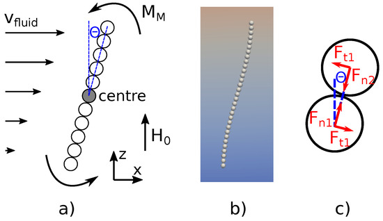
Figure 1.
(a) Linear particle chain model in a fluid flow with homogeneous strain rate . (b) Simulation result of the same problem with our OpenFOAM based solver. (c) Magnetic force between two neighboring particles on the bent chain.
Suppose that initially the chain is vertical and the particles have zero velocity. The fluid then starts to move the chain to the direction x due to the drag force. However, as the fluid has a strain rate, the drag force at the top of the chain is higher than at the bottom section, which causes the chain to start to rotate. As the chain rotates, a counter magnetic torque between the neighboring particle pairs appears due to the magnetic particle–particle interaction. This can be seen more clearly if Equation (8) is rewritten with its tangential and normal components:
where is the angle between the magnetic field and the particle-pair direction; see Figure 1c. The magnetic moments can be expressed with the magnetic field. Based on Equation (4) the moments are proportional to the magnetic field; therefore, the pair force is .
An excellent description of this force and the angle-dependency is presented in [14]. Here only the main consequences are collected based on [14]:
- The normal force between the particles is attractive until . This attractive force is the main reason for the chain formulation.
- The tangential force is 0 at , and it approximately linearly increases with the increasing at small angles.
The chain rotates in the non-homogeneous flow until the torque from the magnetic forces counter-balances the torque of the fluid. Finding the exact rotated shape which is shown in Figure 1b is complicated; therefore, in the follow the chain is considered linear, similarly to a model in [22]. Now the torque of the flow is calculated on the linear chain. First consider the case when the number of particles in the chain is odd. In this case the axis is fixed to the center particle; see Figure 1. We will concentrate to the effect of the upper section of the particles on the center particle. The torque of the ith particle’s drag from the center particle is:
where as all particles have the same velocity, which is equal to the fluid velocity at the center due to the symmetry. In other words, the relative velocity between the particle and the fluid phase is zero at the center. The total torque of the fluid on the chain based on the last two equations is:
The multiplication by 2 has to be done as the bottom section of the chain is also rotated.
The counter torque from the magnetic pair interactions between the neighboring particles can be calculated with Equation (9). For one particle pair the torque is caused by the tangential magnetic force pair, which is shown in Figure 1c. As there are pairs in the chain, the total magnetic torque is:
In the steady rotated chain the net torque is zero; therefore, . By comparing Equation (11) with Equation (12) the tangent of the angle of the steady chain can be calculated as:
The presented equation shows that an increasing strain rate increases the angle. Increasing the magnetic field in turn decreases the angle, as , and in this case the magnetic counter torque becomes higher. Longer chains have a higher rotation angle.
If N is even, i.e., there is no center particle, the torque of the drag in Equation (11) slightly changes, and the summation for i changes to . This has to be applied also for Equation (13). It should be noted that the long chains can be broken over a critical angle; that problem is presented in detail in [22]. In the current work this phenomenon is not investigated.
Using the approximation of , in Equation (13) the magnetic torque for the chain can be rewritten as:
when N is odd, and for the even case, the summation should be changed as described above. This equation shows that we can determine the magnetic torque of the chain from the chain length. The equation can be used to calculate the increased viscosity of the magnetic nanoparticle phase (see later). It can be noted that because of with the increasing chain length, the steady-state magnetic torque is increasing rapidly.
Finally, we also investigated the case when the chain is close to a horizontal wall and one of the chain ends is fixed to it. The fluid velocity is parallel to the wall and its profile is , where z is the distance from the wall. The chain becomes bent due to the drag and the total magnetic torque can be identified with a similar derivation, which is shown above. In this case the total magnetic torque is approximately four times higher for a chain with N particles compared to Equation (14).
3. The Two-Phase CFD Model
A two-phase CFD model was elaborated to handle the nanoparticle aggregation procedure in the magnetic field. The main scope of the work was to create an Euler–Euler-based model, which is able to predict the shape of a macroscopic-sized nanoparticle aggregate in the magnetic field in a fluid flow.
The Euler–Euler-based model considers two-phases: the fluid (phase b) and the nanoparticle phase (phase a). The main issue is the presented micro-chain structure of the nanoparticles, i.e., how the particle–particle magnetic interactions can be treated in a continuous model. Our solution relies on the idea that the effect of the rotated chains in a non-homogeneous flow can be managed as an increased viscosity of the nanoparticle phase. The idea originated from [22]. It should be emphasized that the macroscopic treatment of the micro-chain structure is relevant, as the chain formulation plays the major role in the aggregation. Neglecting the particle–particle interaction in the two-phase model would mean that we do not see any aggregation in the simulation at all, or only at really slow flow rates. In the following section this novel model is presented in detail.
3.1. Governing Equations
The created numerical model is based on the twoPhaseEulerFoam solver in the open source CFD software OpenFOAM v5x [23]. The background of an earlier version of the solver is presented in [24].
In the model, each phase in a computational cell has its own volumetric fraction: and , i.e., in every cell. The volumetric conservation equation for the mixture is
The conservation of the momentum for the fluid is:
where p is the pressure, is the stress tensor, represents the momentum transfer from the other phase and denotes any other source terms. For the particle phase a similar equation can be applied. The stress tensor for the fluid is
where is the identity matrix. For the particle phase a similar form of the stress tensor is applied; however, the value of will be set by a specialized viscosity model considering the effect of the particle chains (see later).
The momentum transfer between the phases is based on the Wen–Yu drag model [25]. This model can be found originally in OpenFOAM for the Eulerian–Lagrangian libraries as a drag model for the particles. The drag force on one particle is calculated as
where is the particle volume; is the Reynolds-number which is calculated as and the function . As in our case , the term in Equation (18) will be approximately 24. It should be noted that the force is equal to the Stokes force when . Converting the particle force to a volumetric force density is done using the simplifications above:
which represents the momentum transfer between the two phases. The magnetic force density of the neodymium magnet on the aggregate phase can be determined from the particle magnetic force, which was shown in Equation (5). Based on this equation and the magnetic moment formula in Equation (2) the magnetic force density is
where the term is caused by the fact that only the core of the particle can be magnetized.
Finally, the phase fraction field is updated by solving the following equation:
and [24].
3.2. Viscosity Model
In the micro-domain model, the rotated chains represent a magnetic torque-density in the aggregate. This phenomenon can be handled as an increased viscosity of the nanoparticle phase. To calculate the viscosity increase, first the magnetic torque density should be determined in the domain. For one chain, the sum of the magnetic torque was presented in Equation (12). The formula can be approximated by Equation (14). The latter provides the magnetic torque if the chain length is known. The problem is that in the two-phase model only the volumetric fraction of the nanoparticle phase is known; i.e., there is no information about the chain lengths in the aggregate. It can be assumed that the chain length distribution depends on the volume fraction of the particles, and also on the magnetic field H. To overcome this problem, several micro-domain simulations were prepared with different nanoparticle concentrations in a given homogeneous magnetic field. In these simulations the particles initially were placed randomly, and then the self-aggregation appeared in the simulations due to the magnetic particle–particle forces. As a result of each simulation, the chain length distribution could be identified at the different concentrations; see more details in the Results section.
Knowing the chain length distribution in a domain, the magnetic torque density can be calculated as
where the summation goes over all chains, and is calculated based on Equation (14). By performing micro-domain simulations at different nanoparticle concentrations, the torque density dependence can be identified. In the next step the magnetic torque density is embedded into the viscosity of the nanoparticle phase. Our numerical implementation is based on OpenFOAM’s Herschel–Bulkey model. First, the strain rate of the nanoparticle phase is calculated explicitly from the previous time step as:
where is the strain rate tensor, and ; i.e., it notes the sum of the product of the tensor components. Then the viscosity of the nanoparticle phase is calculated as
This model follows a relatively simple approach, as the effects of the chains are considered to be isotropic. This method was found to be numerically stable. However, the discussed torque density derivation is only valid when the direction of the chains corresponds to the dominant elements of the strain rate tensor. In our case this condition is roughly true, as at the aggregate-fluid boundary the flow is generally parallel to the boundary. Nevertheless, we intend to improve the model in this aspect in the future.
3.3. Numerical Model
In the original twoPhaseEulerFoam solver the PIMPLE (merged SIMPLE + PISO) segregated algorithm is used to solve the conservation equations. The description of the SIMPLE and PISO algorithms can be found, e.g., in [26]. The phase fraction Equation (21) is solved with OpenFOAM’s MULES (multi-dimensional limiter for explicit solution) algorithm, which is tailored to guarantee the boundedness of the phase fractions.
In viscoelastic problems the SIMPLEC algorithm is preferred [27]. A detailed explanation of the algorithm is presented for one phase in [26,27], and our following description relies on these works. Although the algorithm exists in OpenFOAM, in the two-phase solver twoPhaseEulerFoam it has not been implemented yet.
In our work the SIMPLEC algorithm is embedded into the two-phase solver as follows. Based on the conservation of the momentum, in a new time step the predicted velocity for an arbitrary cell in the mesh can be calculated as:
where is the cell-center velocity value, and denotes the neighboring cell velocities. means any other explicit source terms, while is the pressure from the previous time step. The equation can be written for both phases. As in OpenFOAM the following notations are used:
with those notations the equation can be expressed as
The problem with the guessed velocity fields , is that they do not fulfill the volumetric continuity Equation (15). Therefore, a correction for the velocities and is needed with a new pressure field , whose fields satisfy both Equations (15) and (25):
and
subtracting from Equation (25) to (28) the velocity correction can be expressed with the pressure correction as
In the SIMPLEC algorithm the following approximation is used
i.e., the cell velocity correction is approximated to be the weighted mean of the neighbor corrections. Substituting it into Equation (30):
The volumetric continuity Equation (29) can be rewritten by expressing the velocity corrections with the pressure correction, resulting in the pressure equation. By solving this equation, the pressure correction, i.e., the new pressure field, can be determined. Having these values the velocity corrections for each phase can be calculated using Equation (32). With these the continuity equation, Equation (29), can be rewritten using OpenFOAM’s notation as
by expanding the velocity corrections based on Equation (32):
Finally by expressing the pressure correction as the final form of the pressure equation is
As it was discussed previously, after the new pressure field is calculated, the corrections for the velocities , are obtained by using Equation (32).
In the numerical code the momentum equations (Equation (25)) for both phases were constructed, from which the and terms were obtained. In case of the MNP phase, the changeable viscosity is pre-calculated based on Equation (24), where the local strain rate of the MNP phase is determined from the velocity field of the previous time-step . In the momentum equation of the MNP phase the magnetic force of the magnet in Equation (20) is also included. In the original twoPhaseEulerFoam solver a face-based momentum equation formulation can be chosen, which was also used in our case. From the momentum predictor Equation (27) the and A terms were interpolated to the cell faces as and , and then the guessed phase fluxes through the face are constructed as for both phases, where the f symbol represents the face interpolated values. is the cell face vector, whose magnitude is equal to the face area. According to the original solver the momentum transfer between the phases and the temporal derivative in the momentum equation are included at the calculation of the predicted fluxes. All of the equations after the momentum predictor are expressed with the fluxes.
Another important setting is the boundary condition for the pressure at the fixed velocity boundaries, like at the wall. At the wall both phase velocities are zero; i.e., the total flux going through the wall should be also 0 at the new time step. In the original solver this is achieved by adjusting the pressure gradient boundary condition. This method’s modified version was used in our case. The formula of the total flux with is represented in the pressure equation, where its divergence is set to zero. Based on it, and the known value of the total flux at the boundary the pressure gradient is updated before solving the pressure equation.
4. Experimental Setup
The aggregation procedure was also investigated experimentally. First an appropriate microfluidic device and the MNP suspension were prepared. Then the aggregation procedure was investigated at different flow rates. Finally, thermal measurements were performed both with MNP-filled and MNP-free devices.
4.1. The Microfluidic Chip
In order to verify our model with measurements, first we created a microfluidic structure. The requirement for the device was to be opaque, enabling us to observe the nanoparticle aggregate with a microscope during the aggregation. To reach this goal a unique microfluidic chip was manufactured, which basically consisted of a thin silicon layer between two opaque acrylic plates. The acrylic layers gave the mechanical stability while the silicon layer ensured the sealing. The sketch of the device is shown in Figure 2, while a photo of the device during a measurement is shown in Figure 3. The microfluidic channel was a long rectangular domain, which was cut in the silicon layer. The channel had a uniform width of 4 and its total length was 85 . The thickness of the silica layer, i.e., the height of the channel, was . The three layers were held together by densely placed screws around the channel. The inlet and outlet ports of the channel were drilled through one of the acrylic plates. All the three layers, including the shape of the microchannel, were prepared with laser cutting. The final structure was found robust and stable even after a several days of usage.
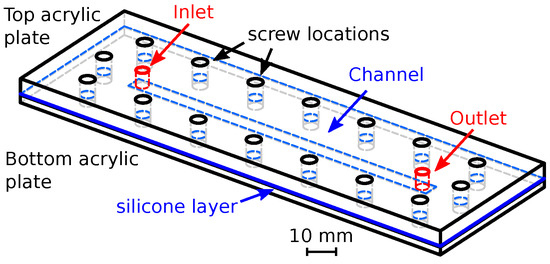
Figure 2.
The schematic of the microfluidic chip. The rectangular channel was cut in a thin, approximately thick silicone layer. The top and bottom surfaces were encapsulated by 4 and 2 thick acrylic plates, respectively. The layers were held together by screws. The channel had a width of 4 . The inlet and outlet ports were drilled through the top acrylic plate.
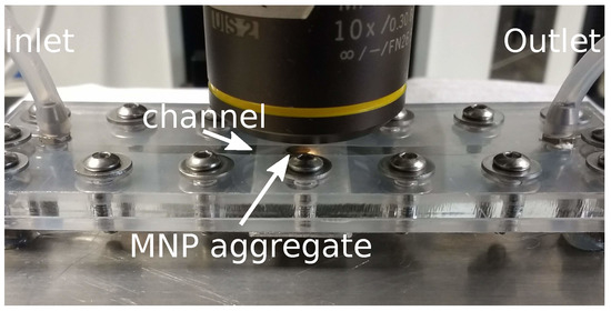
Figure 3.
The photo shows the microfluidic device during a measurement. The MNP suspension continuously flowed thorough the channel from the inlet. A neodymium magnet was positioned under the center of the channel and the nanoparticles aggregated in its magnetic field. The aggregation procedure was monitored with a microscope.
4.2. Magnetic Nanoparticles
The nanoparticles were made of a magnetite core (Fe3O4) which had a diameter of 210 . The core was covered with a 20 thick silicon-dioxide shell, which resulted in a final particle diameter of .
The magnetization curve of the MNPs was investigated in several papers [28,29,30]. Based on these works we concluded that the saturation magnetization of the nanoparticles can decrease as the size decreases with respect to the bulk magnetite saturation magnetization, which is [31]. In our case, however, we were far from the saturation, and therefore in the modeling parts the core was approximated to be linear with the bulk susceptibility of [31].
The nanoparticle suspension was created by mixing the nanoparticles in distilled water. We experienced that the MNP self-aggregation can be significant in the suspension. Polyethylene glycol (PEG) and a small amount of detergent were added to avoid this phenomenon. Using a more diluted suspension, ultrasonic bath and pre-heating of the suspension up to also helped to fragment most of these aggregates.
4.3. Measurement Setup
In the measurements the nanoparticle suspension was forced to flow through the microfluidic channel with different flow rates. The flow control was achieved by using a syringe pump (Fresenius Vial SA Pilote C). A cylindrical neodymium magnet was positioned under the center of the channel with the diameter of and height of . The magnet’s remanent magnetization was according to its datasheet.
To observe the aggregation in the magnetic field the device with the magnet was put under a microscope (Olympus BX51M); see Figure 3.
5. Experimental Results
5.1. Measurement of the MNP Aggregate in the Magnetic Field
The MNP aggregation in the microfluidic channel was studied at different flow rates; the measurement setup is shown in Figure 3. As it was observed, the aggregation started at the bottom wall close to the magnet. According to the expectations, the MNPs were accumulated in chain-like formulations, which were nearly parallel to the magnetic field. The aggregated chains became longer and denser over the time until a steady-state shape was achieved. Photos of the aggregation are shown in Figure 4. It was also noticed that shorter free chains were also developing in the fluid flow, which became longer, as the suspension passed thorough the magnet.
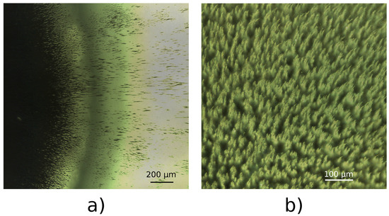
Figure 4.
(a) Microscopic image at the beginning of the aggregation procedure at the end of the aggregate, next to the bottom wall. The contour of the cylindrical magnet is also visible. Most of the MNPs aggregated into a chain-shaped forms, which were nearly parallel to the magnetic field. The fluid flowed from the left to the right. (b) A magnified dark-field image from the top of the steady-state aggregate close to its horizontal center. The ends of the individual aggregate groups are in focus. The fluid flowed from the left to right, which caused the bent shape of the aggregate ends.
The thickness of the nanoparticle aggregate over the magnet was seemingly non-homogeneous. It rather looked to have a spherical surface, deformed by the fluid flow. The maximum thickness of the aggregate was at the center, while at the side walls fewer nanoparticles were aggregated.
To have a comparison of the numerical model and the experiments, the gap between the thickest part of the steady aggregate and the top wall was measured at different flow rates. This was done by manually adjusting the focal point of the microscope. We measured the vertical movement of the microscope between the focus of the top of the aggregate and the top wall of the channel. The channel height was also determined with a similar method, and resulted in . The depth of focus of the objective was 15 .
The aggregation procedure was measured at the different flow rates. Obviously at lower flow rates the quantity of the aggregate was larger because of the reduced drag. In these cases the horizontal shape was more evolved while the aggregate thickness was also higher. The gap sizes between the MNP aggregate and the top wall are presented in Table 1. Note that at the smallest flow rate the top of the aggregate reached the top wall. It should be noted, however, that this was achieved only for a small part at the center of the aggregate, while a small gap still remained for the fluid next to the side walls.

Table 1.
Measurement results of the gap sizes between the top of the MNP aggregate at the center and the top wall at different flow rates. At the lowest flow rate only a small part of the MNP aggregate reached the top wall at the center. In all cases the aggregate was thinner at the side walls than at the center. In the Q = 300 mL h case the aggregate thinning was more representative. The accuracy of the measurement was estimated to .
Finally the volume fraction of the dense nanoparticle phase was measured. A flask was filled with nanoparticle suspension containing 20 of MNP. Then a big neodymium magnet was positioned under the flask, which resulted the MNPs to aggregate to the bottom. After this the MNP-free solvent was removed and the mass of the remaining aggregate with the encapsulated water was measured. Based on this measurement the estimated maximum volume fraction of the nanoparticles was = 11%.
5.2. Thermal Measurements
Thermal measurements with MNP aggregate were also performed at different flow rates, as we were interested in the effect of the MNP aggregate on the thermal characteristics of the microfluidic channel. Pre-heated water was flown through the device first in a MNP-free channel (i.e., when there was no aggregate), and then in an MNP-filled channel. To measure the temperature loss in the chip, temperature sensors were fixed at the ends of the inlet and outlet tubes next to the device; see Figure 5. In the MNP-free channel case the temperature drop was measured at various flow rates. Then the channel was filled with the aggregate, and the temperature loss was measured again. In this case the fluid was the MNP suspension with a concentration of c = 2 mg mL . The thermal measurement at all flow rates started after the steady state shape of the aggregate was achieved. The temperature measurement procedure was started when the inlet-outlet temperature became steady and the given temperature data are the averages of 90 s of measurement.
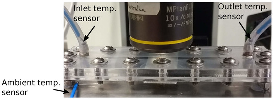
Figure 5.
The figure shows the microfluidic chip prepared for the thermal measurement. Temperature sensors were installed into the inlet and outlet tubes next to the chip. An additional sensor was positioned under the channel to monitor the ambient temperature. The chip with the three sensors sank into icy water during the thermal measurement.
As the expected temperature differences between the two cases are not too high, it was important to perform the experiment in an environment with a fixed temperature. This was achieved by sinking the chip with the tubes in icy water, which provided a constant ambient temperature of . The measured temperatures and their ratios are shown in Table 2. The different inlet temperatures at the different flow rates were caused by the fact that the suspension was also cooled down in the inlet tube, whose end close to the chip was also in the icy water. As was expected, the temperature drop in the chip was higher in case of low flow rates. Moreover, the temperature ratio was consistently smaller in the case of the MNP aggregate’s presence than in case of the MNP-free channel. This shows that the MNP aggregate can be used in the microchannel to enhance the heat transfer. At this stage of the research we cannot determine why the difference was evolved in the temperature. It could be the result of the elevated heat conductivity, the percolation of MNP in magnetic field or the changed flow field. Investigation of this issue can be one focus of future research.
Table 2.
Thermal measurement results with the channel. The table shows the measured inlet and outlet temperatures and their ratio at the different flow rates in the MNP-free and the MNP-filled cases. The accuracy of the K-type thermocouple was ± .
6. Numerical Results
6.1. Modeling the Chain Length Distribution at Different Concentrations
To calculate the magnetic phase’s increased viscosity, the magnetic torque density needs to be identified at different nanoparticle concentrations. It is only an approximation, but by using Equation (22) with Equation (14) it is sufficient to know the chain length distribution to determine the torque density. To calculate it, several micro-domain simulations were accomplished. The numerical solver of the micro-domain model was implemented based on OpenFOAM’s discrete particle method solver DPMFoam. The original solver was extended to calculate the magnetization of the particles and the magnetic interactions between them. In the simulation the particle mass and moment of inertia was calculated by setting the magnetite core density to ρcore = 5250 kg·m−3 and the silicon-dioxide shell density to ρshell = 2196 kg·m−3. The simulation domain was a 20 × 20 × 20 cube, where initially randomly placed particles were positioned. A homogeneous vertical magnetic field was set in the domain. Due to the magnetic field, the particles aggregated into chains, whose direction was parallel to the external magnetic field. The simulations were done at different nanoparticle concentrations: , , , , , and . The formed chains for are shown in Figure 6.
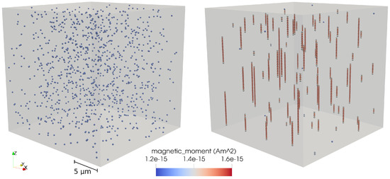
Figure 6.
Aggregation procedure at concentration. The left picture shows the initial random particle positions, the right one shows the self-aggregated structure at . The magnetic field was . The particles are colourised by their magnetic moment values.
To identify the chain length distribution a custom program was written in C++ to post-process the simulation data. In the program the close particles were collected into one group. The chain length was determined based on the difference between the highest and lowest particle positions. This way the chain length distribution and then the torque-density based on Equations (14) and (22) can be calculated algorithmically. By setting the fluid strain rate to and its viscosity to (water’s viscosity) in Equation (14) the average torque densities at the different concentrations were calculated and are shown in Table 3.
Table 3.
Calculated torque densities at different particle concentrations at the fluid strain rate . The torque densities were computed from Equation (22), where each particle chain’s torque was calculated by Equation (14). The particle chain length distributions at the different concentrations were determined based on the micro-domain simulations.
It can be seen that the torque density is rapidly increasing at low concentrations with the increasing concentration. Increasing from to results in approximately three orders of magnitude of change in the torque-density. The reason for this is that at the particle cloud is sparse, and most of the particles are either single or only short chains are formed, containing 2 or 3 particles. The formed chains and particles are far from each other due to the low concentration. In turn at most of the particles are arranged into chains, whose average length is higher than at low concentrations; see Figure 6. Moreover, as it was shown previously the torque of the chains increases approximately with , which results in a rapid change with the increasing chain lengths. The high values of the torque density appear as an increased viscosity of the nanoparticle aggregate, which will help the aggregation.
In the highest investigated concentration the length of the longest chains reached the size of the domain, which was . Over that concentration we assume a linear change of the torque density with the concentration. It should be noted that the evolving chain formulation needs some time to arrange. At lower particle concentrations the time for the arrangement is higher, as initially the particles are further away from each other and the particle–particle force rapidly decreases with distance; see Equation (8). Moreover, the arrangement speed is obviously dependent on the magnetic field strength, as the particle–particle force is approximately proportional with . To find the time when most of the chains are in a stable state, one way is to monitor the total kinetic energy of the particles [14]. After an initial peak this value decreases with time as the particles are arranging into chains. In our case we ran the lowest particle concentration case until . Similarly to [14], by investigating the total kinetic energy of the system we found that at higher particle concentrations the aggregation procedure needed less time.
6.2. Simulation Setup for the Aggregation in the Microchannel
The aggregation in the microchannel was investigated experimentally with a neodymium magnet. In this section the measurement is modeled with the two-phase solver. The local magnetic torque density is determined from Equations (22) and (14), where the chain length distribution term is calculated with a piecewise-linear interpolation, fitted to the 7 results of the micro-domain simulations.
In Equation (14) the fluid’s local strain rate is also needed, which can be identified from the velocity field of the fluid. Due to the magnetic field dependency of the chain length distribution, the torque density was set to , as the magnetic force between the particles is proportional with the square of the magnetic field. It should be noted, however, that this dependency for the chain-length distribution is heuristic and needs further investigation. After the local torque density was calculated, the viscosity of the nanoparticle phase is set as the ratio of the torque density and local strain rate ; see Equation (24).
A two-dimensional simulation was prepared, assuming planar flow in the channel. Although treating the problem in 2D leads to some inaccuracies about the aggregate shape, the computational cost is significantly reduced compared to a 3D case. The simulation domain was a × rectangular domain. The sketch of the simulation domain is shown in Figure 7. At the bottom wall, which was close to the magnet the local magnetic torque density, the MNP phase viscosity was increased to a four-times-higher value compared to Equation (14) according to the discussion of the linear chain model. The fluid phase was water with the density of ρb = 997 kg·m−3 and the viscosity of μb = 8.9 × 10⁻⁴ Pa·s
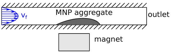
Figure 7.
Sketch of the simulation of the microchannel. The fluid with the nanoparticles flows from the left to the right. The fluid has a parabolic velocity profile. The neodymium magnet is positioned under the center part of the magnet. As the particles arrive in the field of the magnet from the left, they start to aggregate at the bottom wall.
The magnetic field of the neodymium magnet was modeled with a modified version of OpenFOAM’s magneticFoam solver. We extended the code to work on a 2D axisymmetric mesh, as the field of the cylindrical magnet is axisymmetric. This way a higher mesh resolution was achieved with the same computational cost compared to a 3D simulation. The axisymmetric field was mapped to the microchannel using custom code, which was implemented using OpenFOAM’s interpolation classes. The interpolated field in the channel is shown in Figure 8. The magnet was positioned under the center of the simulation domain. The term was also calculated, which was needed to identify the magnetic force on the nanoparticle phase in Equation (20).
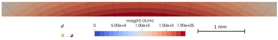
Figure 8.
The calculated magnetic field in the center part of the microchannel. The peak values of the field reach the value of . The lines of induction are also shown.
In the first simulation the fluid and nanoparticle phase velocities at the inlet were set to be parabolic, with a flow rate of Q = 150 mL h , which was one of the used flow rates in the measurements. This flow rate represents an average velocity of in the channel. Zero velocity boundary condition was set for the bottom and top walls for both phases, while at the outlet we used OpenFOAM’s inletOutlet type boundary condition. The pressure was set to at the outlet. At the other boundaries, the gradient of the pressure was set dynamically to fulfill an overall volumetric zero flux before solving the pressure equation, which was discussed in the theoretical section. The volume fraction of the MNP aggregate was set to in the simulation, which means a higher concentration compared to the measurements. This was done in order to speed up the aggregation and reduce the computation times. Based on Table 3, our assumption was that the magnetic torque density is so small at this volume fraction compared to the values at the higher concentrations that this artificial increase will not alter the results of the simulation. Based on [27,32] the convective terms in the momentum equations were discretized with the CUBISTA high-resolution scheme.
The numerical mesh was created with OpenFOAM’s mesh generator blockMesh and it consisted of 86,400 hexahedral elements. It is important to note that the appropriate vertical mesh resolution was crucial to detecting the aggregation. In our case it was set to . Using a rough vertical mesh resolution, e.g., caused the aggregation procedure to be limited to the fluid layers close to the bottom wall. The horizontal mesh resolution was at the center part, while it was less dense at the inlet/outlet, as at these parts no aggregation was expected.
6.3. Results of Modeled Aggregation in the Microchannel
The simulation results showed the aggregation of the nanoparticle phase over the magnet in agreement with the measurements. The main cause of the aggregation was the increased viscosity of the nanoparticle phase. The phase fractions during the aggregation are shown in Figure 9. The aggregation started from the bottom wall over the magnet, similarly to the experiments. Then the aggregate started to grow in both vertical and horizontal directions. As the passage over the aggregate was narrowing over the time, the velocity was increasing here for both phases (see Figure 10), which made the aggregation for the incoming nanoparticles more difficult. Finally, a maximum quantity state was reached, where the gap size did not decrease any more. This means that at the aggregate border there was a balanced state between the drag force and the effect of the increased viscosity. The minimum gap between the top of the aggregate and the top wall was found to be , which is in agreement with the measurement result of ; see Table 1.
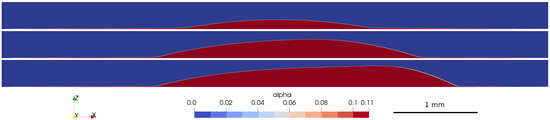
Figure 9.
Nanoparticle phase evolution over the magnet during the aggregation procedure at the flow rate of Q = 150 mL h .
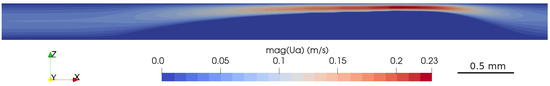
Figure 10.
The velocity field of the nanoparticle phase at the third shown state of the aggregate in Figure 9. The aggregated part has nearly zero velocity, while the fluid with the non-aggregated particle phase bypasses it over the narrow passage.
Simulations were made done at the other flow rates which were used in the measurements. The shapes at the different flow rates are shown in Figure 11. The values of the gap thicknesses are shown in Table 4. At the higher flow rates the gap is larger, as the increased drag force results in less nanoparticles to aggregate.
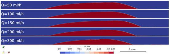
Figure 11.
The simulated aggregate shapes at the different flow rates. As the flow rate is increasing, less MNPs are able to aggregate over the magnet.
Table 4.
The simulated gap heights over the aggregate at different flow rates.
In the simulations we found a dynamic balance rather than a steady shape of the final aggregate. This means that when the aggregate has reached its maximum quantity a small amount from its end was released, and then the filling procedure was repeated until the maximum quantity state was reached again. In Figure 11 the maximum quantity states are shown.
7. Comparison of the Experimental and Numerical Results
The measured and simulated gap heights and their differences at different flow rates are shown in Table 5. It can be seen that the simulated gap heights, and their change with the increasing flow rate corresponds to the measurement results, which shows that the proposed viscosity model relying on the micro-domain simulations can be used to solve such problems. It should be noted, however, that in the measurements at the side walls the aggregate thickness was smaller than at the center. This could be one reason for the difference between the experimental and simulated values.
Table 5.
Gap heights over the aggregate at different flow rates in the simulation. The differences between the measured and simulated gap values based on Table 1 are also presented.
Further Work
The presented two-phase solver is based on the results of the micro-domain simulations. We plan to improve the model by further investigating the magnetic field dependency of the chain distributions in the micro-domain. It should be noted, however, that to identify the exact chain distribution in the microchannel for a given part seems to be a complex problem, as it depends not only on the current MNP concentration and magnetic field, but also on other parameters that would be identified in a more detailed model. The difference between the theoretical micro-domain particles and the real MNPs may also lead to some deviations; i.e., in the model all particles have similar size, while in the reality the particles have a size distribution. The linear chain model itself is also not fully accurate, as is shown in Figure 1. A possible method to bypass the linear chain model is to insert the zero-flow chain distributions in a fluid flow with a constant strain rate, and then monitor the total magnetic torque represented by the magnetic forces between the particles. This way the magnetic torque density can be directly identified from the micro-domain simulation. Moreover, in this case the chain–chain interactions are also included. The viscosity model can be also improved, as was discussed previously. The model can be extended to include the heat transfer, which would be beneficial for the thermal-based applications.
8. Conclusions
In this work a specialized two-phase CFD model and a corresponding solver are presented that are capable of modeling the nanoparticle aggregation in a magnetic field. The model relies on the results of micro-domain simulations, where each particle is modeled separately. These simulations showed that the main reason for the aggregation in micro-scale is the magnetic particle–particle interaction which causes the particles to arrange into chains. The chains in a non-homogeneous fluid flow are bent, resulting in an additional torque-density in the fluid. To investigate the phenomenon a linear chain model is created. Using the model and the particle chain distributions at different MNP concentrations the local torque density of the chains in the fluid flow can be identified. The torque-density calculation was built later in the two-phase model as an increased viscosity. The results show that the torque-density increases rapidly with the increasing concentration of the nanoparticles.
After the micro-domain simulations the two-phase CFD model is presented, wherein the nanoparticles are treated as a second phase in the fluid. Using the two-phase method the simulation of the nanoparticle aggregate became possible in the macro scale. The effect of particle chains in the magnetic field is treated as an increased viscosity. A dedicated solver was created based on the OpenFOAM solver twoPhaseEulerFOAM. In our code the SIMPLEC algorithm was embedded into the two-phase solver, whose solution steps are discussed in detail.
Besides the numerical model, measurements were also performed to verify the simulation results. A microfluidic chip was prepared, containing a wide microchannel. A neodymium magnet was positioned under the channel and a nanoparticle suspension was flown through the channel. The aggregate was formed in the field of the magnet, which was observed with a microscope during the measurement. The aggregation procedure was observed at various flow rates. In all cases the aggregation started at the channel wall close to the magnet and later expanded in both the horizontal and vertical directions until a steady state shape was achieved. The maximum aggregate thicknesses at the different flow rates were measured. Lower flow rates resulted in higher aggregate quantity with a more extended horizontal shape and larger vertical thickness. Thermal measurements were also performed in order to investigate the effect of the aggregate on the heat transfer of the device. Hot water was flown through the channel, and the temperature drop was measured at several flow rates. Then the measurement was repeated using MNP suspension. In all flow rates, the aggregate filled case provided a higher temperature drop. This suggests that the MNP aggregate can be used to increase the heat transfer in the channel.
The two-phase solver was tested by simulating the observed aggregations in the experiment. Although the simulations were run only in 2D, the simulation results generally were in accordance with the measurements. The aggregation procedure in the simulations occurred similarly to the experiments, as the aggregate started to grow from the bottom wall close to the magnet in both vertical and radial directions until a maximum quantity shape. The gap size over the simulated aggregate corresponds to the measured values at the different flow rates.
The presented solver was able to give a prediction of the shape of the nanoparticle aggregate. This shows that the model can be used in the applications using magnetic nanoparticles and may be a useful novel tool in the design procedures of such devices.
Author Contributions
Conceptualization, P.P., M.N. and M.R.; methodology, P.P. and M.N.; software, P.P.; validation, P.P. and M.N.; writing—original draft preparation, P.P., M.N. and M.R.; writing—review and editing, P.P., M.N. and M.R.; supervision, M.R. All authors have read and agreed to the published version of the manuscript.
Funding
The research work was supported by the New National Excellence Program of the Ministry for Innovation and Technology of Hungary, financed from the National Research, Development and Innovation Fund of Hungary (ÚNKP-20-4-I). The research work was supported by the National Research, Development and Innovation Fund of Hungary (Budapest, Hungary; project SNN-125637). The research reported in this paper and carried out at the Budapest University of Technology and Economics was supported by the “TKP2020, Institutional Excellence Program” of the National Research Development and Innovation Office in the field of Artificial Intelligence (BME IE-MI-SC TKP2020).
Conflicts of Interest
The authors declare no conflict of interest.
Nomenclature
| General notation | scalar, vector |
| magnetic field [ ], [ ] | |
| magnetization [ ] | |
| magnetic moment of particle i [ ] | |
| p | pressure [ ] |
| Q | flow rate [ ] |
| velocity [ ] | |
| volume fraction | |
| strain rate [ ] | |
| dynamic viscosity [ ] | |
| density [ ] | |
| magnetic torque density [ ] | |
| magnetic susceptibility | |
| volumetric flux on a face [ ] | |
| CFD | computational fluid dynamics |
| MNP | magnetic nanoparticle |
References
- Fan, J.; Gao, Y. Nanoparticle-supported catalysts and catalytic reactions–a mini-review. J. Exp. Nanosci. 2006, 1, 457–475. [Google Scholar] [CrossRef]
- Ender, F.; Weiser, D.; Nagy, B.; Bencze, C.L.; Paizs, C.; Pálovics, P.; Poppe, L. Microfluidic multiple cell chip reactor filled with enzyme-coated magnetic nanoparticles—An efficient and flexible novel tool for enzyme catalyzed biotransformations. J. Flow Chem. 2016, 6, 43–52. [Google Scholar] [CrossRef]
- Weiser, D.; Bencze, L.C.; Bánóczi, G.; Ender, F.; Kiss, R.; Kókai, E.; Szilágyi, A.; Vértessy, B.G.; Farkas, Ö.; Paizs, C.; et al. Phenylalanine Ammonia-Lyase-Catalyzed Deamination of an Acyclic Amino Acid: Enzyme Mechanistic Studies Aided by a Novel Microreactor Filled with Magnetic Nanoparticles. ChemBioChem 2015, 16, 2283–2288. [Google Scholar] [CrossRef] [PubMed]
- Pálovics, P.; Ender, F.; Rencz, M. Towards the CFD model of flow rate dependent enzyme-substrate reactions in nanoparticle filled flow microreactors. Microelectron. Reliab. 2018, 85, 84–92. [Google Scholar] [CrossRef]
- Pálovics, P.; Ender, F.; Rencz, M. Geometric optimization of microreactor chambers to increase the homogeneity of the velocity field. J. Micromech. Microeng. 2018, 28, 064002. [Google Scholar] [CrossRef]
- Ahrberg, C.D.; Manz, A.; Chung, B.G. Polymerase chain reaction in microfluidic devices. Lab Chip 2016, 16, 3866–3884. [Google Scholar] [CrossRef] [PubMed]
- Sosnovik, D.E.; Nahrendorf, M.; Weissleder, R. Magnetic nanoparticles for MR imaging: Agents, techniques and cardiovascular applications. Basic Res. Cardiol. 2008, 103, 122–130. [Google Scholar] [CrossRef]
- Reddy, L.H.; Arias, J.L.; Nicolas, J.; Couvreur, P. Magnetic nanoparticles: Design and characterization, toxicity and biocompatibility, pharmaceutical and biomedical applications. Chem. Rev. 2012, 112, 5818–5878. [Google Scholar] [CrossRef]
- Das, P.; Colombo, M.; Prosperi, D. Recent advances in magnetic fluid hyperthermia for cancer therapy. Colloids Surf. B Biointerfaces 2019, 174, 42–55. [Google Scholar] [CrossRef]
- Gui, N.G.J.; Stanley, C.; Nguyen, N.T.; Rosengarten, G. Ferrofluids for heat transfer enhancement under an external magnetic field. Int. J. Heat Mass Transf. 2018, 123, 110–121. [Google Scholar]
- Goharkhah, M.; Salarian, A.; Ashjaee, M.; Shahabadi, M. Convective heat transfer characteristics of magnetite nanofluid under the influence of constant and alternating magnetic field. Powder Technol. 2015, 274, 258–267. [Google Scholar] [CrossRef]
- Lajvardi, M.; Moghimi-Rad, J.; Hadi, I.; Gavili, A.; Isfahani, T.D.; Zabihi, F.; Sabbaghzadeh, J. Experimental investigation for enhanced ferrofluid heat transfer under magnetic field effect. J. Magn. Magn. Mater. 2010, 322, 3508–3513. [Google Scholar] [CrossRef]
- Li, Q.; Xuan, Y. Experimental investigation on heat transfer characteristics of magnetic fluid flow around a fine wire under the influence of an external magnetic field. Exp. Therm. Fluid Sci. 2009, 33, 591–596. [Google Scholar] [CrossRef]
- Han, K.; Feng, Y.; Owen, D. Three-dimensional modelling and simulation of magnetorheological fluids. Int. J. Numer. Methods Eng. 2010, 84, 1273–1302. [Google Scholar] [CrossRef]
- Karvelas, E.; Lampropoulos, N.; Sarris, I.E. A numerical model for aggregations formation and magnetic driving of spherical particles based on OpenFOAM®. Comput. Methods Programs Biomed. 2017, 142, 21–30. [Google Scholar]
- Boutopoulos, I.D.; Lampropoulos, D.S.; Bourantas, G.C.; Miller, K.; Loukopoulos, V.C. Two-Phase Biofluid Flow Model for Magnetic Drug Targeting. Symmetry 2020, 12, 1083. [Google Scholar] [CrossRef]
- Ghaffari, A.; Hashemabadi, S.H.; Bazmi, M. CFD simulation of equilibrium shape and coalescence of ferrofluid droplets subjected to uniform magnetic field. Colloids Surfaces A Physicochem. Eng. Asp. 2015, 481, 186–198. [Google Scholar] [CrossRef]
- Jackson, J.D. Classical Electrodynamics; John Wiley & Sons: Hoboken, NJ, USA, 2012. [Google Scholar]
- Guyon, E.; Hulin, J.P.; Petit, L.; Mitescu, C.D. Physical Hydrodynamics; Oxford University Press: Oxford, UK, 2001. [Google Scholar]
- Saliba, A.E.; Saias, L.; Psychari, E.; Minc, N.; Simon, D.; Bidard, F.C.; Mathiot, C.; Pierga, J.Y.; Fraisier, V.; Salamero, J.; et al. Microfluidic sorting and multimodal typing of cancer cells in self-assembled magnetic arrays. Proc. Natl. Acad. Sci. USA 2010, 107, 14524–14529. [Google Scholar]
- Bossis, G.; Volkova, O.; Lacis, S.; Meunier, A. Magnetorheology: Fluids, structures and rheology. In Ferrofluids; Springer: Berlin, Germany, 2002; pp. 202–230. [Google Scholar]
- Martin, J.E.; Anderson, R.A. Chain model of electrorheology. J. Chem. Phys. 1996, 104, 4814–4827. [Google Scholar] [CrossRef]
- Weller, H.G.; Tabor, G.; Jasak, H.; Fureby, C. A tensorial approach to computational continuum mechanics using object-oriented techniques. Comput. Phys. 1998, 12, 620–631. [Google Scholar] [CrossRef]
- Rusche, H. Computational Fluid Dynamics of Dispersed Two-Phase Flows at High Phase Fractions. Ph.D. Thesis, University of London, London, UK, 2002. [Google Scholar]
- Wen, C.Y. Mechanics of fluidization. Chem. Eng. Prog. Symp. Ser. 1966, 62, 100–111. [Google Scholar]
- Ferziger, J.H.; Perić, M.; Street, R.L. Computational Methods for Fluid Dynamics; Springer: Berlin, Germany, 2002; Volume 3. [Google Scholar]
- Pimenta, F.; Alves, M. Stabilization of an open-source finite-volume solver for viscoelastic fluid flows. J.Non-Newton. Fluid Mech. 2017, 239, 85–104. [Google Scholar] [CrossRef]
- Rajput, S.; Pittman, C.U., Jr.; Mohan, D. Magnetic magnetite (Fe3O4) nanoparticle synthesis and applications for lead (Pbr2+) and chromium (Cr6+) removal from water. J. Colloid Interface Sci. 2016, 468, 334–346. [Google Scholar] [CrossRef]
- Goya, G.; Berquo, T.; Fonseca, F.; Morales, M. Static and dynamic magnetic properties of spherical magnetite nanoparticles. J. Appl. Phys. 2003, 94, 3520–3528. [Google Scholar] [CrossRef]
- Daoush, W. Co-precipitation and magnetic properties of magnetite nanoparticles for potential biomedical applications. J. Nanomed. Res. 2017, 5, 1–6. [Google Scholar] [CrossRef]
- Thompson, R.; Oldfield, F. Magnetic properties of natural materials. In Environmental Magnetism; Springer: Berlin, Germany, 1986; pp. 21–38. [Google Scholar]
- Pimenta, F.; Alves, M. rheoTool. 2016. Available online: https://github.com/fppimenta/rheoTool (accessed on 21 May 2020).


© 2020 by the authors. Licensee MDPI, Basel, Switzerland. This article is an open access article distributed under the terms and conditions of the Creative Commons Attribution (CC BY) license (http://creativecommons.org/licenses/by/4.0/).