Abstract
The paper assumes that, at the end of the operational period of a Spanish nuclear power plant, an Independent Spent Fuel Storage Installation will be used for long-term storage. Spent fuel assemblies are selected and transferred to casks for dry storage, with a series of imposed restrictions (e.g., limiting the thermal load). In this context, we present a variant of the problem of spent nuclear fuel cask loading in one stage (i.e., the fuel is completely transferred from the spent fuel pool to the casks at once), offering a multi-start metaheuristic of three phases. (1) A mixed integer linear programming (MILP-1) model is used to minimize the cost of the casks required. (2) A deterministic algorithm (A1) assigns the spent fuel assemblies to a specific region of a specific cask based on an MILP-1 solution. (3) Starting from the A1 solutions, a local search algorithm (A2) minimizes the standard deviation of the thermal load among casks. Instances with 1200 fuel assemblies (and six intervals for the decay heat) are optimally solved by MILP-1 plus A1 in less than one second. Additionally, A2 gets a Pearson’s coefficient of variation lower than 0.75% in less than 260s CPU (1000 iterations).
1. Introduction
Optimization problems are found at different levels in electric power systems, from both technological and operations management standpoints. In transport and distribution, not intending to make an exhaustive list, there are studies related to classical modeling and problem solving for electric energy distribution static planning [1,2,3]; other works, also on planning, propose a flexible distribution attending to the emerging variability of demand [4]. There are also many examples of optimization problems at the source point, from renewable generation (see for instance [5] for wind) to nuclear power.
A nuclear power plant is a complex system in which many optimization processes take place. The balance between safety requirements, competition in a liberalized electricity market, and access to limited human and material resources is resolved in nuclear power plants through an approach that prioritizes safety (see, for instance, INSAG-4 [6] and IAEA-TECDOC-1329 [7]).
Nuclear Power Plants (NPP) produce electricity from the heat released in a fission chain reaction; the so-called “nuclear fuel” is actually fissionable material. In Light Water Reactors (LWR), the type of reactor that constitutes the majority of the world’s nuclear fleet and the total of the Spanish fleet [8], nuclear fuel is made of uranium (slightly enriched in the 235U isotope), in the form of ceramic pellets of UO2 protected and waterproofed by a metallic cladding (zirconium alloy) and grouped together, forming the so-called fuel assemblies (FA) [9]. The fuel used in the two units of Ascó NPP (the plant that has inspired the present study) is manufactured by ENUSA under a license agreement with Westinghouse, the owner of the technology [10].
Presently, the two Ascó units have fuel burn-up cycles of one and a half year. Each 18 months, some 60 FA (out of the 157 contained in the core of the reactor) are replaced (each one containing about 500 kg of uranium). Up to the end of its service, each Spent Fuel Assembly (SFA) has produced around 50 GWd/t of heat.
In the fission process, uranium atoms are transformed into radioactive fission products. Roughly speaking, in an SFA, some 5% of the initial uranium mass has undergone fission. A smaller part of the uranium is also transformed, through neutron capture nuclear reactions, into transuranic elements, which are also radioactive. The hazard of spent fuel is due to the potentially harmful effects of ionizing radiation. Thus, it is necessary to isolate the spent fuel for a long time to avoid the dispersion of the radioactive substances. An ultimate storage solution is proposed in repositories excavated in deep geological formations [11], in a way similar to that followed with chemical contaminants such as mercury [12].
The decay of radioactive substances in the spent fuel causes the so-called “decay heat”, which decreases as the activity of those substances declines, but which requires careful management of SFAs to prevent them from being damaged by excess temperature. After being removed from the core of the reactor, spent fuel is temporarily stored in the fuel pool of each power unit. Pool water provides shielding and cooling. Only when the power of the SFA has been sufficiently reduced can it be considered for dry storage in appropriate containers (either temporarily or permanently in a deep geological repository). The lack of political consensus for a definitive solution in Spain made it necessary to propose a Central Interim Storage Facility (CISF) [13], which was never built (now, it is proposed for 2028 [14]).
Over time, the spent fuel pools of the Spanish NPP have been reaching the limit of their capacity. In the case of the two units of Ascó, the pool in each of them can house 1421 FA, which is a figure that includes the 157 positions needed to discharge the entire reactor core if necessary. At the end of 2018, there were 1160 FAs in the Ascó 1 pool and 1104 in the Ascó 2 pool. The plant has 608 SFAs in an Independent Spent Fuel Storage Installation (ISFSI) in 19 HI-STORM containers [15], each hosting 32 SFAs [16].
In Spain, ENRESA (a state-owned company) is responsible for the decommissioning of the nuclear installations, as well as for the ultimate disposal of nuclear and radioactive wastes [17]. At the end of the exploitation period, it is in the interest of the plant operator to be able to transfer ownership of the installation to ENRESA in the shortest possible time. In order to do it, previously, all the fuel must be completely removed from the spent fuel pool [18]. At this moment, the ISFSI can be used as a logistics storage, housing spent fuel containers prior to transportation to the CISF. If the CISF is not yet available, the ISFSI should be usable as a full-scope storage (perhaps even in the long-term).
Thus, an optimization problem arises: it is necessary to remove all of the SFA from the pool within the minimum time and at the minimum cost [19]? Indeed, optimization problems can be found in a wide variety of operations in NPPs. For instance, in the spent fuel pool, where the SFAs are stored in racks, problems arise in optimizing the reliability of the design of the racks and the arrangement of the assemblies in the event of their possible displacement [20], and, as the capacity of the pool is limited to a specific number of assemblies, other management problems of spent nuclear fuel storage arise linked to this limitation [21]. At the right time, SFAs are removed from the pool and relocated in casks, often for long-term storage. The optimization here ranges from determining the SNF removal allocation strategy for a fleet of plants [22], to the design of the containers (e.g., what capacity, how much cooling time needed, etc.) [23], to the strategies to be followed in the loading of the casks.
As for the latter, Zerovnik et al. [24] propose combinatorial methods to optimize the cask loading, aiming at final geological repository. Considering as well the final deposition, Ranta and Cameron [25] used a two-phase heuristic method in order to minimize the thermal load of the canister with the largest load. Gomes et al. [26] propose a methodology, using genetic algorithms, to determine the optimal time to load the casks for dry interim storage, taking into account several cost factors. Spencer et al. [27] have develop a method (embedding greedy randomized adaptive search procedures in a memetic algorithm) to optimize the cask loading in a multi-objective search of configurations that minimize the number of casks, the thermal load, and the time when the transportation requirements are met.
In the present work, the cask loading problem is solved with two hierarchical optimization criteria: (i) minimize the cost of the regionalized casks necessary to relocate the spent fuel located in the pool at a given moment [28] using mixed integer linear programming [29]; and (ii) minimize the standard deviation of the thermal load in the set of casks using a multi-start metaheuristic with local search procedures [30].
In Section 2, we describe some dry storage systems for spent nuclear fuel. Section 3 is devoted to the description, modeling, and resolution of the spent nuclear fuel cask loading problem. Section 4 illustrates the procedure proposed in a case study inspired in Ascó NPP. Finally, Section 5 provides the conclusions derived from this work and a brief description of future research lines.
2. Dry Storage Systems for Spent Nuclear Fuel
Different solutions exist for the interim dry storage of spent nuclear fuel; as a comparison, the 14 closed sites in the USA use 11 different storage systems from four different suppliers [31].
In Spain, ENRESA has adopted different solutions. Some plants are using dual-purpose containers (transport and storage) whose structure provides shielding, confinement, and heat dissipation. Ascó’s two units are using the multi-purpose HI-STORM system, which is described below [15,16].
The spent fuel storage and transport system in Ascó is made up of different elements: the multi-purpose canister (MPC-32), the storage module (HI-STORM), the transport overpack (HI-STAR), and the transfer cask (HI-TRAC), which allows the MPC to be transferred to HI-STORM and HI-STAR [15] (see Figure 1).
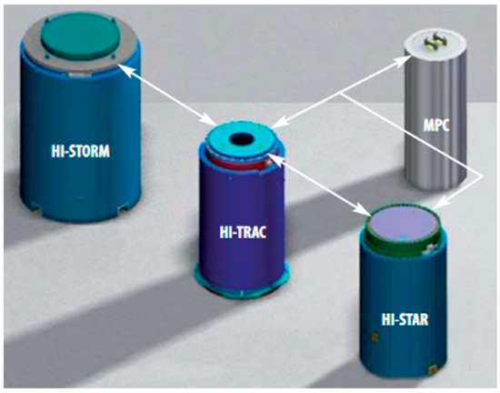
Figure 1.
Components of the HI-STORM system for the storage and transportation of spent nuclear fuel. The HI-TRAC transfer cask allows the MPC to be transferred to the HI-STORM and HI-STAR [15].
The time required to completely remove the spent fuel from the pool depends on the minimum cooling time necessary for the last SFA to be loaded into a cask. This cooling period (that is, the time elapsed since the unload of the SFA from the reactor core) depends, in turn, on the type of container used and the technical specifications approved by the regulator for it.
To guarantee the integrity of the SFAs, the temperature of the metal cladding that surrounds the UO2 pellets must be limited. This fact imposes requirements of sufficient heat dissipation in the cask design. However, also, it imposes a limit to the thermal power that the SFAs can generate inside the cask. For instance, in the HI-STORM system, under uniform charging conditions, each of the positions of the MPC-32 can house an SFA with a maximum power of 0.9375 kW at the time of loading (i.e., the total thermal power dissipated by the canister will be limited to 30 kW) [32]. The system allows regionalized loads; so, SFAs with higher decay heat can be located in the central region of the canister (region , formed by 12 positions), at the cost of limiting the maximum power per position in the peripheral region (region , 20 positions) and also limiting the total thermal load to a value less than 30 kW [33]. Figure 2 represents the positions assigned to each region.
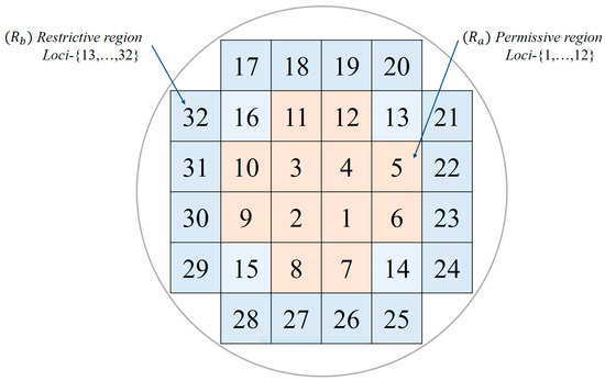
Figure 2.
Cross-section of a regionalized MPC-32, showing the positions of the permissive region and the restrictive region (inspired from Holtec).
In fact, the loading of a cask is constrained by the technical specifications in a more complex way, since they take into account, in addition to the cooling time, multiple fuel characteristics such as decay heat, burn-up, initial enrichment, the possibility that the assembly has some damage, or the possible presence of elements such as neutron sources, control rods, burnable poisons, etc. These conditions vary according to the type of cask, its use (storage or transport), and other specific limitations.
In what follows, it is assumed that at the end of the operational life of the plant, an ISFSI will exist that allows transfering all of the SFAs to it using the HI-STORM system (without imposing the present transport requirements, which are more restrictive than storage requirements). It is considered here that the storage requirements apply only to the decay heat of each SFA (calculated in turn from the burn-up, cooling time, and initial enrichment). The minimum time for the complete removal of all of the SFA from the pool is bounded by the moment when the hottest SFA fits into the requirements. The cost will depend on the number of containers to be used. So, the number of containers needed to remove all the SFA from the spent fuel pool needs to be minimized: this is the optimization problem addressed in the present study.
3. The Spent Nuclear Fuel Cask Loading Problem
In this section, we describe and formalize the spent nuclear fuel cask loading problem, and we propose a hybrid metaheuristic to solve it. Our method works in three phases using mixed integer linear programming (MILP), a deterministic algorithm, and local search heuristics.
3.1. Description of the Problem
At a given instant , corresponding to the planned date for transferring in one go the contents of the spent fuel pool to the ISFSI, there are SFAs, forming a set ()).
At the time of removal, T, each fuel assembly is characterized by a thermal power (decay heat), .
On the other end, there is an ISFSI ready to host all of the casks needed. Casks are regionalized, i.e., they are compartmentalized into regions with attributes of capacity and decay heat. Thus, there is a set of virtual regions ( (, in which each type of region is characterized by the upper and lower bounds on the decay heat a single SFA may have , and the number of SFAs in that region that can be held by a single cask, . symbolizes the type of universal region capable of housing any fuel assembly without restrictions.
There is a set ( ( of cask classes; symbolizes the universal class, which is capable of accommodating any fuel assembly without restrictions at an arbitrary high cost . Each class is defined in relation to the maximum thermal load allowed in each region of the cask.
An adversity coefficient is associated to each class of cask , corresponding to the arbitrary cost of selecting a cask of class to house at least one SFA. We also assume for the class a maximum number of units available, . The total number of available casks is .
The relationship between a virtual region type and a cask class is given by matrix , whose coefficients take the value 1 when the region of type is associated to the cask of class , and 0 otherwise.
On the other hand, the relationship between the fuel assembly and the type of region is given by matrix , whose coefficients, , are equal to 1 when the fuel assembly can be located in the region at time , and 0 in any other case; i.e., . It follows from it that the relationship between the fuel assembly and the class of cask is given by matrix resulting from the boolean product of matrices and ; that is, , thus fulfilling the following property: .
Under such conditions [28], the spent nuclear fuel cask loading problem consists of transferring the maximum number of the fuel assemblies, which are located in the pool of a nuclear power plant on a date and expressed as time after the end of operation, into a set of regionalized casks of different classes, meeting the restrictions and minimizing costs (i.e., minimizing the total adversity).
3.2. Solving the Problem
As discussed above, our proposal solves the problem in three phases. The first phase uses MILP to allocate fuel assemblies to virtual regions with minimum cost (i.e., a minimum number of casks or minimum total adversity) [28]. In the second phase, a family of deterministic algorithms has been designed to assign each SFA to a specific cask actual region. Finally, in the third phase, a local search heuristic is proposed to minimize the standard deviation of the thermal load of the casks set.
3.2.1. Phase 1: MILP Model to Minimize the Cask Loading Cost
To formalize the proposed resolution methods, we use the following nomenclature.
Parameters:
| Time or expected date to remove in one go the SFA from the pool in the nuclear power plant, expressed as time after the end of operation. | |
| Set of SFA located in the pool of the nuclear power plant at time . Let the elements be (). | |
| Set of virtual region types according to the upper and lower bounds on the decay heat of the SFAs. Let the regions be with . The universal region, , does not impose any limit; for practical purposes, the assigned elements to the universal region will remain in the pool. | |
| Set of classes of casks: with . The type of cask considered here corresponds to MPC-32 described above. We will assume that there is a type of universal container, , associated with the universal region ; for practical purpose, the elements assigned to the universal container will remain in the pool. | |
| Decay heat of the fuel assembly at the time . | |
| Upper limit of a single SFA’s decay heat in the virtual region . | |
| Lower limit of a single SFA’s decay heat in the virtual region type . Here, we will assume . | |
| Element–region compatibility matrix; technological coefficients equal to 1 if the fuel assembly can be located in the virtual region at time , and 0 otherwise. Formally: . | |
| Region-cask compatibility matrix; technological coefficients equal to 1 if the region of type is associated with the cask class , and 0 otherwise. | |
| Element–cask compatibility matrix, which is defined as ; technological coefficients are equal to 1 when the element can be placed in a cask of class at time , and 0 otherwise. Therefore, it is true that: . | |
| Storage capacity of a region of type measured by the number of SFAs a single cask can hold in that region at most. | |
| Maximum storage capacity of a cask of class measured by the number of fuel assemblies. The relationship is fulfilled. | |
| Number of available casks of the class at time . The expected total cask availability is . | |
| Adversity coefficient for a cask of class . The value symbolizes the arbitrary cost if a cask of class is selected to hold SFAs. |
Variables:
| Binary variable that equals 1 if the fuel assembly is assigned to the virtual region , and 0 otherwise. | |
| Number of fuel assemblies assigned to the virtual region . | |
| Number of casks of class . | |
| Total adversity function. It represents the overall cost of the casks used to hold the spent nuclear fuel on the scheduled date, , after the pool of the nuclear power plant is emptied. |
Using these parameters and variables, we formulate the following mathematical model.
MILP-1: Model for the assignment of fuel assemblies to types of virtual region
Subject to:
In the MILP-1 model, the objective Function (1) represents the minimization of the cask loading cost or total adversity, whose value coincides with the total number of casks when all the fuel assemblies are removed from the pool and the adversity coefficients are unitary for any class of cask . Equalities (2) and (3) guarantee the assignment of all the fuel assemblies to any region, including the universal region . Equality (4) determines the number of fuel assemblies that must be assigned to each type of region . Constraint (5) lower bounds the number of casks of each class , while Constraint (6) upper bounds that value according to their availability. Condition (7) imposes that the decision variables are binary and, finally, the non-negativity and integrity of the auxiliary variables and are given by (8) and (9), respectively.
Running the MILP-1 model offers three types of results: (i) an optimal assignment of the fuel assemblies to the various virtual regions , (ii) the optimal number of SFA assigned to each region , and (iii) the optimal number of casks of each class corresponding to the minimum cost.
Although the previous results are interesting, the location of the fuel assemblies in the real regions of the casks remains to be determined.
3.2.2. Phase 2: Assignment of the Fuel Assemblies to the Real Cask Regions
Any sequence of objects corresponding to the triplet of sets can lead to a different solution. For example, if the sequence is built on the set of fuel assemblies, then the number of different ways to assign is This can lead to an astronomical number of potentially different solutions for instances of realistic dimensions (e.g., in our case study). Based on this idea, we propose a family of constructive algorithms, ], which depends on the regulatory sequence of the assignment of fuel assemblies to virtual regions.
Starting from an optimal solution given by MILP-1, the procedure creates a sequence of fuel assemblies (Statement 5 in ) to establish the sequence of assignment of SFAs to casks. Once the procedure determines the class of the cask that corresponds to the current element , the element is recorded in the matrix (Statement 13 in ), whose rows correspond to casks and whose columns correspond to positions within the cask. Subsequently, the heat loads in the casks are determined (Statement 16 in ), and the elements are sequenced in the casks according to such loads (Statement 17 in ). Finally, the results of the algorithm are returned (Statement 18 in ).
| Algorithm 1.: Algorithms to assign fuel assemblies to regions according to |
|
Note that Algorithm 1 can generate many solutions thanks to the fact that the starting point is a permutation of the fuel assemblies of the set (Statement 5 in ). Such permutations can be created using a family of rules applied on the set , which is initially ordered according to the SFA’s identifier (). The family of rules can be of diverse nature; they may consist of the same initial sequence (lexicographic order) or the simple sequence of the elements according to the decay heat or in more complex rules used for the generation of neighborhoods (exchange and insertion) in algorithms based on trajectories through the search domain.
Obviously, all the solutions generated by are optimal when the function objective is the minimization of the cost of the casks [28], as happens in Phases 1 and 2 of this work; however, when the objective function corresponds to another optimization criterion, such as the balancing of the heat load in the set of casks, can be used in, at least, two ways:
- (1)
- In the construction phase (or phases) of multi-start algorithms, v.gr. greedy randomized adaptive search procedure (GRASP) algorithms, to build initial solutions to be used as seeds for the next phase of trajectory-based improvement in the search domain.
- (2)
- In the systematic generation of solutions, to assist metaheuristics based on populations (v.gr. genetic and memetic algorithms).
In this work, Algorithm 1 constitutes one of the fundamental pillars for the construction of initial solutions, and the chosen way is (1).
3.2.3. Phase 3: Reduction of the Dispersion of the Thermal Load of the Casks
Phase 3 of the proposed procedure aims to reduce, by a predetermined number of iterations, the dispersion of the thermal load (measured in kW) in the set of casks. The dispersion metric to minimize chosen here is the standard deviation ; this is:
where:
| Total optimal number of casks: . It is obtained by applying the MILP-1 procedure by setting values to the adversity coefficient ). | |
| Total thermal load due to the SFA loaded on date in the -th cask of class : . These values are obtained after applying the Algorithm 1 by fixing a permutation of the elements of set . | |
| Average value of the thermal load in the set of casks on date : | |
| Standard deviation of the thermal load in the set of casks on date . |
In order to carry out Phase 3, the non-exhaustive descent Algorithm 2 is applied, based on local search optimization (see Algorithm 2 below). Its main characteristics are as follows.
Phase 3.1: Initialization of Algorithm 2
- An initial solution is obtained, applying the mathematical program MILP-1, after prefixing the values of the vector ) of adversity coefficients; this solution is characterized by the triple of sets of values .
- The Algorithm 1 is applied to the solution , considering the arbitrary sequence , which initially corresponds to : the lexicographic order of the SFA’s identifiers (). Thus, the extended solution is obtained, which contains detailed information on the location of each element inside the casks in the matrix .
- Solution is fixed as the incumbent solution of the local search iterative procedure . In addition, is fixed as the best solution , and the standard deviation of this solution is determined.
Phase 3.2: Improvement of the initial solution with
- A tentative solution belonging to the restricted neighborhood of the incumbent solution is generated—that is, —where is the rule for generating neighboring solutions and is the set of possible solutions. Specifically, given the incumbent solution , the generation rule operates as follows: for all pairs of different casks and all pairs of positions in these casks , the tentative neighboring solutions exchange the elements between these positions, within the set of possible solutions that is regulated by the SFA–cask compatibility matrix .
- If the tentative solution is a possible solution ( and , then the solution becomes the best solution and also the new incumbent solution .
- The above steps are repeated within Phase 3.2 as long as there is an improvement to the incumbent solution or the number of tentative solutions generated does not reach the preset value (v.gr. tentative solutions).
| Algorithm 2.: Non-exhaustive local search descent algorithm based on |
|
3.2.4. Multi-Start Metaheuristics Assisted by Assignment Sequences
The proposed metaheuristic integrates the procedures of the three phases described above (see Schema . This metaheuristic can be classified within the category of multi-start algorithms, since it uses a multitude of initial solutions generated by the algorithm of Phase 2. In the generation of solutions, uses a current sequence string ; this chain is progressively constructed by moderately altering the current sequence giving rise to the next ongoing permutation. The main characteristics of are the following:
- The Algorithm 3 metaheuristic is initialized by executing Phase 3.1, starting with an initial solution offered by MILP-1 (Phase 1) and registering the sequence as an assignment current sequence; that is: .
- In a specific iteration, given an arbitrary current sequence, which we will denote as , the algorithms and are cascaded, making , and thus obtaining a solution that is locally optimal.
- In an iteration, to go from an ongoing assignment current sequence to the next current sequence , there are many alternatives. Specifically, in this work, we have chosen to apply a slight mutation on the first sequence . This mutation, characterized by the rule, consists of exchanging, in pairs, the fuel elements located in four positions of the current sequence chosen at random.
- Thus, for each , the number of initial solutions locally optimized by is equal to the number of sequences generated with the mutation rule. The procedure ends when the number of mutated sequences reaches a maximum value equal to (v.gr. mutate sequences).
| Algorithm 3.Metaheuristic: Three-Phase Hybrid Metaheuristics Based on and |
|
4. Case Study
This section is dedicated to a case study inspired in the spent fuel pools of Ascó NPP (Tarragona, Spain). It contains the following points: (i) the model assumptions, (ii) the requirements for spent fuel cask loading, (iii) the procedures used, (iv) the data used, and (v) the results achieved.
4.1. Hypothesis for the Case
The following hypotheses are assumed for the case at hand:
Hypothesis 1 (H1).
Fuel assemblies are characterized by their type, burn-up (), initial enrichment (% by mass), and the time elapsed since they are unloaded from the core (in years). From these data, the decay heat of each element can be determined at the time it is transferred from the pool to the cask.
Hypothesis 2 (H2).
There are no fuel assemblies damaged or affected by other additional constraints.
Hypothesis 3 (H3).
The elements associated with the fuel, such as neutron sources, control rods, consumable poisons, and others, are not considered in the model.
Hypothesis 4 (H4).
It is assumed that only one type of cask is available in terms of physical dimensions and number of positions for fuel assemblies, the MPC-32.
Hypothesis 5 (H5).
The fuel assemblies are loaded into the casks taking into account the requirements for storage in module-type HI-STORM storage containers. It is assumed that there is no capacity limit in the ISFSI.
Hypothesis 6 (H6).
The contents of the spent fuel pool at the end of the operation of the plant (T = 0) are assumed to be known. To carry out the case study, the real content of the spent fuel pool of NPP Ascó 1 is used here. The decay heat of each of the SFA at any given time T can be computed from their cooling time (this is T plus the time each SFA has previously spent in the pool) and the SFA’s burn-up and initial enrichment.
Hypothesis 7 (H7).
The pool should be emptied using the minimum possible number of casks on the earliest possible date. The date has been chosen as T = 6 years in order to guarantee that even the hottest SFA meets the requirements.
Hypothesis 8 (H8).
It may be interesting that the thermal load of the casks is balanced. Therefore, we aim at minimizing the standard deviation of the thermal load of the set of casks.
4.2. Requirements for the Storage of Fuel Assemblies
The requirements to take into account for emptying the pool are as follows:
- R1.
- Casks are of the MPC-32 type, which are compartmentalized in 32 positions, each one containing a single fuel assembly (see Figure 2).
- R2.
- The positions of a MPC-32 are grouped into two regions: () a permissive region with a high limit for the decay heat formed by positions and () a restrictive region with a low limit for the decay heat formed by positions.
- R3.
- A fuel encapsulation position (concept for which we will use the Latin noun locus–loci) can house an SFA whose cooling time is greater than 5 years (in our case, with T = 6 years, this does not constitute any limitation).
- R4.
- The contents of each locus in any cask must have a decay heat less than or equal to the maximum allowed in the locus: in region and in region .
- R5.
- The maximum heat load allowed in a cask is equal to .
- R6.
- The maximum values for decay heat at loci are determined according to the case:
- -
- Case of uniform loading: the maximum decay heat allowed per locus in the MPC-32 equals (30 ). Therefore, if all SFAs have a decay heat , then only one class of container is needed, and the problem has a trivial solution (in what concerns the minimization of the number of casks)
- -
- Case of regionalized loading: if any SFA has a decay heat , then some casks allowing regionalized load are needed. In this case, the maximum values of decay heat per locus ( or ) according to the region to which it belongs ( o ) are determined as follows:
- (1)
- Set a value of the ratio of the maximum values of decay heat per locus , such that ( corresponts to the uniform loading, is the maximum value allowed by the regulator for this ratio).
- (2)
- Determine the maximum allowed thermal load per locus, for the restrictive region , from the expression:where is a function bounded to 1 for and decreasing with . The function for the MPC-32 is:
- (3)
- Determine the maximum allowed thermal load per locus, for the permissive region :
4.3. Data and Other Characteristics of the Case
Obviously, the dimensions of the MILP-1 model are a function of the instances used. In this work, we use the ASCÓ#01_6.0 instance (see Table A1 in Appendix A) as data for decay heat. The main characteristics of the experiment are as follows:
- (1)
- The number of spent fuel assemblies is equal to . The elements are identified with the indices corresponding to the first natural numbers.
- (2)
- The expected date for the removal of elements from the pool is years after the end of operation. The decay heat values listed in Table A1 of Appendix A correspond to years.
- (3)
- The number of virtual regions of decay heat is equal to . Let be those regions that are defined with closed intervals of decay heat per locus. The regions are specified from three values of the ratio of maximum thermal loads: . Let:
For convenience, virtual regions have been numbered in descending order of the upper limit of each interval.
- (1)
- The definition of virtual regions ( to ) allows establishing the element–region compatibility matrix , whose technological coefficients adopt the value 1 if the fuel assembly can be assigned to a virtual region of type at the time , and 0 otherwise. Formally:
- (2)
- The number of cask classes is if we omit the neutral virtual region r0, which corresponds to the pool. The correspondence between the virtual regions ( to ) and the real classes of the regionalized cask ( a C) is established through the region-cask compatibility matrix , whose coefficients are equal to 1 when the region is associated with cask , and they are 0 otherwise. In our case, matrix is as follows:
Thus, a cask is compartmentalized in a permissive region with the characteristics of and a restrictive region associated with a cask is associated with a permissive region and another restrictive ; and finally, a cask has only one region with the qualities of the intermediate region r3.
- (1)
- From a technological point of view, all the containers in this study correspond to MPC-32, with 12 positions in the permissive region and 20 positions in the restrictive regions. Obviously, an MPC-32 of class has 32 positions in the unique region.
- (2)
- Taking into account that the number of cask classes is , it remains to define the unit cost per each class. In order to measure the impact of the adversity coefficients on the solutions offered by MILP-1, different values are given to the arbitrary costs ).
- (3)
- Taking into account the values and characteristics exposed in the previous points, the dimensions of the MILP-1 model for the Ascó # 01_6.0 instance are the following: (i) 6984 binary decision variables corresponding to the assignment of fuel assemblies to virtual regions; (ii) 6 integer variables associated with the number of fuel assemblies hosted by each virtual region; (iii) 4 representative integer variables () for the number of casks of each class; and (iv) 1195 constraints (1199 if the availability of casks is bounded).
4.4. Procedures
All compiled codes corresponding to the procedures used have been executed on a DELL Inspiron-13 (Intel(R) Core(TM) i7-7500U @ 2.70 GHz CPU 2.90 GHz, 16 GB de RAM, x64 Windows 10 Pro). The models and tools used to find the optimal solutions for this case study are the following:
- (1)
- Model MILP-1 [28] based on MILP that allows minimizing the cost of the containers required to transfer all the SNF from the NPP pool. MILP-1 also offers the number of SFAs assigned to each region as well as an optimal assignment of each SFA to a virtual region. For the exploitation of MILP-1, we use the IBM ILOG CPLEX solver (Optimization Studio v.12.2, win-x86-64).
- (2)
- Deterministic method that starts from the result of MILP-1 and offers an assignment of SFAs to the permissive and restrictive regions of the casks based on the sequence of assignment of SFAs to casks . Here, 1000 consecutive allocation sequences are considered, which are generated by slightly mutating one of them to obtain the next, following the neighborhood transition rule . MILP-1 plus (with lexicographic order of the fuel assembly codes) constitute the deterministic procedure proposed in [28].
- (3)
- Local search heuristic that starts from a solution generated by and explores neighborhoods non-exhaustively until reaching a local optimum. The procedures MILP-1 plus plus (with the mutation rule applied to the sequence in iterations) constitute the metaheuristic proposed in this work.
In short, metaheuristic works in this manner: from an optimal solution found by MILP-1, which is characterized by the triple of sets of values , the algorithm is applied times, transferring one by one and following sequences , the SFAs assigned to the virtual regions ( toward the physical regions (permissive and restrictive) of the casks , using the region-cask compatibility matrix . Afterwards, the local optimization corresponding to heuristics is applied to all solutions generated by algorithm .
4.5. Results
In addition to considering the solution from MILP-1 with the triplet , which corresponds to minimizing the total number of casks, and in order to assess the impact of the adversity coefficients on the solutions offered by MILP-1, 24 other optimal solutions are also analyzed, fixing the list of arbitrary costs ) to the following values:
Using the deterministic procedure proposed in [28], after obtaining an optimal solution with MILP-1 , the algorithm is applied following the sequence corresponding to the lexicographic order of the fuel assembly identifiers. The global results of the 25 solutions are shown in Table 1.

Table 1.
Summary of results of the 25 optimal initial solutions (#0 to #24) provided by procedure proposed in [28] for the Ascó #01_06 instance with the following technical characteristics: (i) 1164 Spent Fuel Assemblies (SFAs), (ii) T = 6 years, (iii) 6 virtual regions (including the neutral region) defined by three values of the ratio (1, 2, and 3), and (iv) 4 cask classes (including the neutral container).
Specifically, in Table 1, the following data are collected for each solution (#0 to #24):
- (1)
- The cost ) imputed to each cask class.
- (2)
- The optimal number of casks of each class and the total number ) of casks required by each solution.
- (3)
- The optimal values of the objective cost function for the MILP-1 model.
- (4)
- The average thermal load corresponding to the configuration of each solution .
- (5)
- The standard deviation of the thermal load in the set of casks: .
Table 1 shows 16 optimal solutions that require 37 MPC-32, which is a number that also coincides with the minimum number of casks, according to the lower bound (). However, these solutions show different values of the standard deviation of the thermal load, depending on the configuration of the 37 casks.
As an example, initial solution #9, one with the lowest thermal load dispersions between the casks: , corresponds to the triplet of costs , in which it is considered that the adversity to the use of casks of classes and is 1.5 times higher that of class casks.
Based on solution #9, the FAs column in Figure 3 shows the number of SFAs assigned to each virtual region, i.e., . This is translated into a total requirement of 37 casks (see the MPC[zk, hj] column in Figure 3), and regionalized casks of classes , , and , respectively.
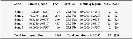
Figure 3.
Solution #9 (MILP-1): number of fuel assemblies and casks in each virtual region.
On the other hand, Figure 4 shows the detailed loads of the containers MPC-32 number n.1 (class ), number n.3 (class ) and number n.26 (class ) of the initial solution #9. These loads are characterized by the identifiers and decay heat of the fuel assemblies located in each MPC-32.
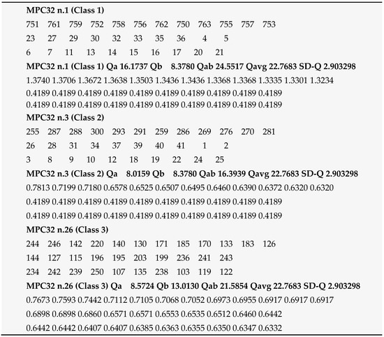
Figure 4.
Initial solution #9 ( proposed in [28]): identifier and decay heat of the SFAs contained in the MPC-32 with identifying numbers n.1, n.3, and n.26.
In view of Figure 4, the following can be stated:
- Cask n.1 of initial solution #9 is class with a permissive region of 12 positions and a restrictive region of 20. The 12 hottest assemblies in this cask are located in region , so locus-1 is occupied by the fuel assembly 751 with a decay heat of 1.3740 kW, while the fuel assembly 753 (the last in ) is located in locus-12 with 1.3234 kW. Complementarily, 20 “cold” elements are located in positions 13 to 32 of the restrictive region of MPC-32 n.1, assembly 23 in locus-13, and assembly 21 in locus-32, whose decay heats are 0.4189 kW, coinciding with the decay heat of all the elements located in this region.
- Casks n.3 (initial solution #9) is class , with its permissive region and its restrictive region . In region , the 12 hottest elements of this cask are located with element 255 occupying locus-1 and element 281 located in locus-12 with residual heats equal to 0.7813 kW and 0.6320 kW, respectively. In addition, all the SFAs located in the restrictive region are considered to have a decay heat of 0.4189 kW.
- Finally, cask n.26 of initial solution #9 is class 3 with a uniform region consisting of 32 positions: . The loci-{1,12,13,32} are occupied by the elements 244, 126, 144, and 122, their respective decay heats being as follows: 0.7673, 0.6917, 0.6898, and 0.6332 kW.
Other interesting results shown in Figure 4 are as follows: (i) the total thermal load casks n.1, n.3, and n.26, which are 24.55, 16.39, and 21.59 kW, respectively; (ii) the thermal loads in the permissive and restrictive regions of these casks (v.gr. in MPC-32 n.26: 8.57 and 13.01 kW); (iii) the average thermal load, equal to 22.77 kW, corresponding to the load of the 1164 SFAs in the 37 casks that constitute initial solution #9; and, finally, (iv) the standard deviation of the thermal load associated with initial solution # 9, .
On the other end, to illustrate the performance of the metaheuristic in terms of improving the standard deviation of the thermal load in the set of casks, nine solutions have been selected from the 25 solutions presented in Table 1. The solution selection criterion meets the following conditions:
- (1)
- Have a total number of containers that is minimal; that is: .
- (2)
- If two or more solutions with , have the same configuration of containers by type , the one that presents smaller standard deviation is chosen; for example, between solutions #2 and #9, we select solution #9.
The final solutions selected to apply Phase 3 to improve using metaheuristic are shown in Table 2. The indicators selected to compare these solutions are as follows: (i) the standard deviations and corresponding to the initial solutions provided by and the improved solutions provided by , (ii) the iteration corresponding to the best solution with ; (iii) the computing time in seconds, , corresponding to the iteration ; and (iv) the computing time in seconds, , given to to improve 1000 initial solutions provided by from a solution provided by MILP-1.
Table 2.
Summary of results of the solutions selected to apply Phase 2 plus Phase 3 of the proposed procedure . The table shows the values: , , , , and .
In view of Table 2, we can draw the following conclusions:
- (1)
- Metaheuristic uses on average 632 s of CPU time to reach the best local optimum of 1000 initial solutions from algorithm . This average is included in the range of values [511, 729] in seconds.
- (2)
- Metaheuristic takes on average 254.4 s of CPU time to obtain the best solution (locally optimized) from 1000 initial solutions generated by . This average is included in the range of values [7.9, 652.3] in seconds.
- (3)
- On average, the iteration (best solution using ) is (over 1000 iterations). This average is included in the range of values [10, 998] in iterations.
- (4)
- The procedure proposed in [28] obtains, on average, solutions with a standard deviation of the thermal load equal to . The range of values for is [2.90, 3.52].
- (5)
- On average, the metaheuristic proposed in this work obtains solutions with a standard deviation of the thermal load of the set of casks equal to , from the solutions generated by and the rule The range of values for is [0.0001, 0.5464].
- (6)
- On average, the standard deviation is reduced approximately 20 times by applying the metaheuristic versus procedure proposed in [28].
To illustrate the reduction in the dispersion of the thermal load in the set of casks, Figure 5 shows the detailed loads of the containers MPC-32 number n.1 (type ), number n.3 (type ), and number n.22 (type ) from solution #10 provided by metaheuristic .
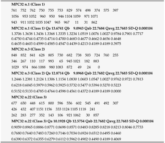
Figure 5.
Improved solution #10 (: identifier and decay heat of the SFAs contained in MPC-32 with identifying numbers n.1, n.3, and n.22.
Figure 6 and Figure 7 show graphically the thermal loads corresponding to the solutions provided by procedure proposed in [28] (see Figure 6) versus metaheuristic proposed in this work (see Figure 7) for each region (permissive and restrictive) and for each of the 37 casks. Note the significant differences that exist between the thermal loads of the 37 used MPC-32 in both figures, despite the fact that the containers present the same thermal limitation characteristics number by number (1 to 37).
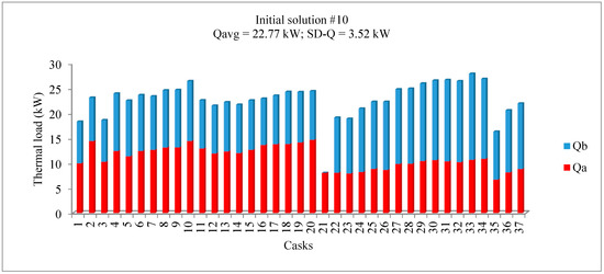
Figure 6.
Solution #10 ( [28]): thermal loads for each of the 37 used MPC-32 as an addition of the ones in the permissive (Qa) and restrictive (Qb) regions.
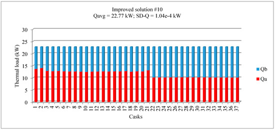
Figure 7.
Solution #10 (metaheuristic ): thermal loads for each of the 37 used MPC-32 in addition to the ones in the permissive (Qa) and restrictive (Qb) regions.
In addition, Appendix B contains the detailed configurations of the 37 containers corresponding to solution #10 provided by metaheuristic .
5. Conclusions
A hybrid multi-start procedure assisted by mixed integer linear programming and local search optimization algorithms, that we have called here metaheuristic , has proven to be competitive in solving the spent fuel cask loading problem with minimal storage cost and a minimum standard deviation of thermal load. This is confirmed through the experiments carried out with the database of Ascó NPP. It allows generating instances with industrial dimensions (e.g., 1200 fuel assemblies and from 1 to 30 classes of regionalized casks, which translates into a number of decay heat virtual regions between 2 and 60).
The method proposed here, , to solve the single-stage cask loading of spent nuclear fuel is computationally competitive in its three phases: MILP-1 mathematical program, deterministic algorithm , and local search heuristic algorithm .
(i) The MILP-1 model is used to minimize the cost of casks required to host the nuclear fuel; it offers, as a solution, an optimal assignment of fuel assemblies to virtual thermal regions, in less than 0.5 CPU seconds, using instances with 1200 fuel assemblies, 6 types of regions, and 4 classes of casks. (ii) Algorithm , which starts from an MILP-1 solution, can assign the SFAs to the real regions of the casks in less than 0.25 s for the tested instances. (iii) The local search algorithm based on 1000 initial solutions generated by by slight mutations of the sequences, is capable of reducing the initial values of the standard deviation 20 times compared to the solutions provided by [28], in an average CPU time equal to 4.24 min.
In other words, metaheuristic (made up MILP-1 plus plus ) is capable of obtaining, on average, a solution with a Pearson’s coefficient of variation lower than 0.75% in less than 260s CPU (1000 iterations). In the slowest approximation, obtains a solution with a Pearson’s coefficient of variation lower than 2.4%, starting from around 15.5% in little more than 12 min CPU (1000 iterations).
Future working lines taking advantage of these results include the following: (1) the formulation and exploitation of other models based on MILP for the regionalized cask loading according to several optimization criteria, and (2) the extension of the above models and procedures to the multi-stage load case.
Author Contributions
Conceptualization, J.B.-V. and L.B.; methodology, J.B.-V.; software, J.B.-V.; validation, J.B.-V., L.B. and M.M.; formal analysis, J.B.-V., L.B. and M.M.; investigation, J.B.-V., L.B. and M.M.; resources, J.B.-V., L.B. and M.M.; data curation, J.B.-V. and L.B.; writing—original draft preparation, J.B.-V.; writing—review and editing, J.B.-V., L.B. and M.M.; visualization, J.B.-V., L.B. and M.M.; supervision, J.B.-V., L.B. and M.M.; project administration, J.B.-V. and L.B.; funding acquisition, J.B.-V. and L.B. All authors have read and agreed to the published version of the manuscript.
Funding
This research received no external funding.
Acknowledgments
This work has been subsidized by the Ministry of Science, Innovation and Universities of the Government of Spain with the OPTHEUS project (ref. PGC2018-095080-B-I00), including Funds for European regional development, and the UPC project “Tool development for the simulation and optimization of the emptying of spent fuel pools in nuclear power plants” financed by ENDESA Generation. The authors also thank the Asociación Nuclear Ascó–Vandellós II (ANAV) the support provided and, especially, to Jordi Estrampes, head of Reactor Engineering and Nuclear Safeguards at NPP Ascó, for his tips and clarifications.
Conflicts of Interest
The authors declare no conflict of interest.
Nomenclature
| CISF | Central Interim Storage Facility |
| IAEA | International Atomic Energy Agency |
| INSAG | International Nuclear Safety Group |
| ISFSI | Independent Spent Fuel Storage Installation |
| LWR | Light Water Reactor |
| MILP | Mixed Integer Linear Programming |
| NPP | Nuclear Power Plant |
| SFA | Spent Fuel Assembly |
Appendix A. Instance Ascó#01_06
Table A1.
Set of SFAs corresponding to the Ascó instance #01_6.0. The characteristics are as follows: identifier of the element, corresponding to row x and column y. The values in the table correspond to the decay heat (in kW) for years.
Table A1.
Set of SFAs corresponding to the Ascó instance #01_6.0. The characteristics are as follows: identifier of the element, corresponding to row x and column y. The values in the table correspond to the decay heat (in kW) for years.
| x\y | 1 | 2 | 3 | 4 | 5 | 6 | 7 | 8 | 9 | 10 |
|---|---|---|---|---|---|---|---|---|---|---|
| 0 | 0.4189 | 0.4189 | 0.4189 | 0.4189 | 0.4189 | 0.4189 | 0.4189 | 0.4189 | 0.4189 | 0.4189 |
| 10 | 0.4189 | 0.4189 | 0.4189 | 0.4189 | 0.4189 | 0.4189 | 0.4189 | 0.4189 | 0.4189 | 0.4189 |
| 20 | 0.4189 | 0.4189 | 0.4189 | 0.4189 | 0.4189 | 0.4189 | 0.4189 | 0.4189 | 0.4189 | 0.4189 |
| 30 | 0.4189 | 0.4189 | 0.4189 | 0.4189 | 0.4189 | 0.4189 | 0.4189 | 0.4189 | 0.4189 | 0.4189 |
| 40 | 0.4189 | 0.4189 | 0.4189 | 0.4189 | 0.4189 | 0.4189 | 0.4189 | 0.4189 | 0.4189 | 0.4189 |
| 50 | 0.4189 | 0.4189 | 0.4189 | 0.5979 | 0.5841 | 0.5789 | 0.5789 | 0.5962 | 0.5818 | 0.6080 |
| 60 | 0.5384 | 0.6084 | 0.5310 | 0.5766 | 0.5732 | 0.5784 | 0.6014 | 0.5801 | 0.5562 | 0.5721 |
| 70 | 0.5766 | 0.5477 | 0.5704 | 0.5477 | 0.5835 | 0.5302 | 0.5484 | 0.5318 | 0.5749 | 0.6098 |
| 80 | 0.6098 | 0.6098 | 0.5789 | 0.6010 | 0.5772 | 0.5236 | 0.5302 | 0.5302 | 0.5772 | 0.6049 |
| 90 | 0.5962 | 0.6101 | 0.5302 | 0.4772 | 0.4820 | 0.4756 | 0.4836 | 0.4740 | 0.4836 | 0.4756 |
| 100 | 0.4756 | 0.5335 | 0.6350 | 0.5979 | 0.6296 | 0.5962 | 0.6385 | 0.5997 | 0.5962 | 0.5979 |
| 110 | 0.5335 | 0.5997 | 0.5979 | 0.5962 | 0.6860 | 0.5351 | 0.5962 | 0.5940 | 0.6347 | 0.6010 |
| 120 | 0.6296 | 0.6332 | 0.6296 | 0.5927 | 0.5335 | 0.6917 | 0.6898 | 0.6165 | 0.6147 | 0.7068 |
| 130 | 0.4942 | 0.6183 | 0.6917 | 0.4925 | 0.6363 | 0.4942 | 0.4909 | 0.4958 | 0.4974 | 0.7105 |
| 140 | 0.4925 | 0.7442 | 0.6112 | 0.6898 | 0.4974 | 0.5875 | 0.5451 | 0.5853 | 0.5343 | 0.5401 |
| 150 | 0.5335 | 0.5451 | 0.5858 | 0.5444 | 0.5318 | 0.5418 | 0.5434 | 0.5910 | 0.5905 | 0.5841 |
| 160 | 0.5789 | 0.5302 | 0.5858 | 0.5335 | 0.5351 | 0.5327 | 0.5434 | 0.5418 | 0.5302 | 0.6955 |
| 170 | 0.7052 | 0.5055 | 0.5039 | 0.5813 | 0.5088 | 0.5270 | 0.5844 | 0.5064 | 0.5253 | 0.5031 |
| 180 | 0.5072 | 0.5270 | 0.6917 | 0.5831 | 0.6973 | 0.5023 | 0.5253 | 0.5848 | 0.5990 | 0.5467 |
| 190 | 0.5973 | 0.5533 | 0.5973 | 0.5500 | 0.6571 | 0.6571 | 0.5417 | 0.5417 | 0.6535 | 0.6094 |
| 200 | 0.5533 | 0.5973 | 0.6553 | 0.5939 | 0.5500 | 0.6025 | 0.5533 | 0.5550 | 0.6007 | 0.5384 |
| 210 | 0.6172 | 0.5351 | 0.6154 | 0.5360 | 0.6154 | 0.5394 | 0.5477 | 0.5236 | 0.6101 | 0.7112 |
| 220 | 0.5484 | 0.6119 | 0.5360 | 0.6154 | 0.5236 | 0.5494 | 0.5351 | 0.5477 | 0.5368 | 0.5410 |
| 230 | 0.5351 | 0.6137 | 0.6101 | 0.6442 | 0.6303 | 0.6512 | 0.6165 | 0.6355 | 0.6407 | 0.6233 |
| 240 | 0.6460 | 0.6442 | 0.6442 | 0.7673 | 0.6028 | 0.7593 | 0.6285 | 0.6079 | 0.6199 | 0.6407 |
| 250 | 0.5977 | 0.6233 | 0.6216 | 0.6407 | 0.7813 | 0.6199 | 0.6062 | 0.6477 | 0.6495 | 0.6079 |
| 260 | 0.6425 | 0.6390 | 0.6477 | 0.6045 | 0.6045 | 0.6407 | 0.6045 | 0.6285 | 0.6390 | 0.6320 |
| 270 | 0.6320 | 0.6355 | 0.6320 | 0.6355 | 0.6337 | 0.6372 | 0.6355 | 0.6407 | 0.6251 | 0.6372 |
| 280 | 0.6320 | 0.6337 | 0.6372 | 0.6442 | 0.6512 | 0.6460 | 0.7199 | 0.7180 | 0.6543 | 0.7238 |
| 290 | 0.6507 | 0.6490 | 0.6525 | 0.6525 | 0.6472 | 0.6490 | 0.6507 | 0.6454 | 0.6454 | 0.6578 |
| 300 | 0.6543 | 0.6525 | 0.7753 | 0.7793 | 0.7117 | 0.7117 | 0.7733 | 0.7713 | 0.7097 | 0.7203 |
| 310 | 0.7184 | 0.7165 | 0.7241 | 0.6923 | 0.7184 | 0.6923 | 0.6904 | 0.7260 | 0.7165 | 0.7203 |
| 320 | 0.7184 | 0.7203 | 0.6904 | 0.7184 | 0.7146 | 0.7071 | 0.7128 | 0.7071 | 0.7109 | 0.7090 |
| 330 | 0.7071 | 0.7109 | 0.7034 | 0.7222 | 0.7165 | 0.7146 | 0.7128 | 0.6757 | 0.6794 | 0.6775 |
| 340 | 0.6794 | 0.6757 | 0.6775 | 0.6775 | 0.6757 | 0.6218 | 0.4535 | 0.6261 | 0.6261 | 0.4566 |
| 350 | 0.6244 | 0.6279 | 0.4520 | 0.6289 | 0.6244 | 0.4489 | 0.6307 | 0.6783 | 0.6915 | 0.6839 |
| 360 | 0.6802 | 0.6972 | 0.6839 | 0.6991 | 0.6915 | 0.8315 | 0.8274 | 0.8336 | 0.8315 | 0.8212 |
| 370 | 0.8336 | 0.8233 | 0.8482 | 0.9784 | 0.9710 | 0.9759 | 0.9858 | 0.9735 | 0.9784 | 0.9759 |
| 380 | 0.9883 | 0.7239 | 0.7182 | 0.7258 | 0.7239 | 0.8357 | 0.8357 | 0.7599 | 0.7638 | 0.7677 |
| 390 | 0.8315 | 0.7658 | 0.7638 | 0.7638 | 0.7638 | 0.7284 | 0.7717 | 0.7638 | 0.7343 | 0.7323 |
| 400 | 0.8441 | 0.7304 | 0.7677 | 0.7677 | 0.7658 | 0.7658 | 0.7483 | 0.7386 | 0.7638 | 0.7463 |
| 410 | 0.7483 | 0.7483 | 0.7521 | 0.7502 | 0.7560 | 0.7463 | 0.7463 | 0.7502 | 0.7502 | 0.7463 |
| 420 | 0.7406 | 0.7776 | 0.7736 | 0.7795 | 0.7677 | 0.7680 | 0.7720 | 0.7620 | 0.7560 | 0.7640 |
| 430 | 0.7540 | 0.7640 | 0.7640 | 0.8666 | 0.8558 | 0.8623 | 0.8623 | 0.8558 | 0.8710 | 0.8688 |
| 440 | 0.8820 | 0.8952 | 0.8864 | 0.8886 | 0.8908 | 0.8842 | 0.8908 | 0.8886 | 0.9063 | 0.7704 |
| 450 | 0.7644 | 0.7724 | 0.7704 | 0.7882 | 0.7700 | 0.7720 | 0.7781 | 0.7744 | 0.7781 | 0.7680 |
| 460 | 0.7943 | 0.7923 | 0.7882 | 0.7842 | 0.7903 | 0.7842 | 0.7903 | 0.7882 | 0.7903 | 0.8579 |
| 470 | 0.7680 | 0.7720 | 0.8601 | 0.8514 | 0.7700 | 0.7761 | 0.8492 | 0.7903 | 0.7923 | 0.7943 |
| 480 | 0.7903 | 0.8128 | 0.7801 | 0.8086 | 0.8066 | 0.8046 | 0.8256 | 0.8128 | 0.8107 | 0.7882 |
| 490 | 0.8213 | 0.8046 | 0.7903 | 0.8149 | 0.8087 | 0.8192 | 0.7882 | 1.0027 | 0.9203 | 0.9955 |
| 500 | 0.9955 | 0.9249 | 1.0027 | 0.9180 | 0.9111 | 0.9180 | 0.9295 | 0.9931 | 0.9907 | 0.9835 |
| 510 | 0.9157 | 0.9157 | 0.9835 | 1.1306 | 1.1223 | 1.1278 | 1.1389 | 0.8030 | 0.8997 | 0.8907 |
| 520 | 0.8030 | 0.7968 | 0.9134 | 0.8974 | 0.8134 | 0.8303 | 0.8345 | 0.8367 | 0.8345 | 0.8303 |
| 530 | 0.8113 | 0.8134 | 0.8197 | 0.8093 | 0.8155 | 0.8218 | 0.8218 | 0.8303 | 0.8093 | 0.8155 |
| 540 | 0.8239 | 0.8261 | 0.8197 | 0.8134 | 0.8218 | 0.8439 | 0.8218 | 0.8527 | 0.8351 | 0.8197 |
| 550 | 0.8395 | 0.8197 | 0.8155 | 0.8218 | 0.8218 | 0.8483 | 0.8460 | 0.8373 | 0.8197 | 0.8218 |
| 560 | 0.8460 | 1.0201 | 0.7901 | 1.0176 | 1.0126 | 0.7989 | 1.0226 | 0.7814 | 0.7836 | 0.7923 |
| 570 | 0.7879 | 1.0126 | 1.0151 | 1.0076 | 0.7901 | 0.7749 | 1.0201 | 1.0076 | 1.0026 | 1.0026 |
| 580 | 1.0026 | 0.8483 | 0.8329 | 0.8329 | 0.8417 | 0.8395 | 0.8505 | 0.8329 | 0.8549 | 0.8615 |
| 590 | 0.8483 | 0.8527 | 0.8571 | 0.8460 | 0.8505 | 0.8571 | 0.8571 | 0.8929 | 0.8816 | 0.8839 |
| 600 | 0.8839 | 0.8285 | 0.8929 | 0.8861 | 0.8460 | 0.8351 | 0.8351 | 0.8839 | 0.8907 | 0.8771 |
| 610 | 0.8549 | 0.8727 | 0.8727 | 0.9916 | 0.8771 | 0.8549 | 0.8549 | 0.8615 | 0.9890 | 0.8749 |
| 620 | 0.8794 | 0.8704 | 0.9994 | 0.9890 | 0.8749 | 1.1196 | 1.1168 | 1.1306 | 1.1141 | 1.0868 |
| 630 | 1.0439 | 1.0814 | 1.0652 | 1.0519 | 1.0733 | 1.0281 | 1.0412 | 1.0439 | 1.0333 | 1.0733 |
| 640 | 1.0679 | 1.0652 | 1.0412 | 1.0254 | 1.0733 | 1.1196 | 1.1278 | 1.1168 | 1.1278 | 0.8965 |
| 650 | 0.8872 | 0.8895 | 0.8942 | 0.8895 | 0.8918 | 0.8965 | 0.8918 | 0.9036 | 0.8965 | 0.8918 |
| 660 | 1.0679 | 1.2543 | 1.0706 | 1.0679 | 1.2575 | 0.9106 | 1.2381 | 0.9083 | 1.0599 | 1.0760 |
| 670 | 0.9083 | 1.0706 | 1.0572 | 1.0652 | 0.8965 | 1.2543 | 0.9059 | 0.9036 | 0.9012 | 0.9059 |
| 680 | 0.9130 | 1.0603 | 0.9036 | 0.9177 | 0.9130 | 0.9059 | 0.9201 | 0.9012 | 0.8989 | 1.2510 |
| 690 | 1.2543 | 0.9012 | 1.2380 | 1.1614 | 1.2502 | 1.2336 | 1.1614 | 1.2367 | 1.1526 | 1.1496 |
| 700 | 1.1555 | 1.2428 | 1.2367 | 1.2306 | 1.2306 | 1.1585 | 1.1485 | 1.2367 | 0.9433 | 0.9408 |
| 710 | 0.9383 | 0.9408 | 0.9584 | 1.1233 | 1.1175 | 0.9534 | 0.9458 | 1.1146 | 1.1204 | 0.9508 |
| 720 | 0.9762 | 0.9609 | 0.9660 | 0.9762 | 1.0716 | 0.9788 | 0.9559 | 1.0859 | 1.0802 | 1.0830 |
| 730 | 0.9635 | 0.9813 | 1.0631 | 0.9839 | 1.0631 | 1.0575 | 0.9788 | 1.0547 | 0.9813 | 0.9762 |
| 740 | 0.9762 | 0.9813 | 1.0547 | 1.0660 | 1.0547 | 0.9890 | 0.9788 | 1.0603 | 0.9640 | 1.3368 |
| 750 | 1.3740 | 1.3638 | 1.3234 | 0.9775 | 1.3335 | 1.3436 | 1.3301 | 1.3503 | 1.3672 | 0.9721 |
| 760 | 1.3706 | 1.3436 | 1.3368 | 0.9667 | 1.0631 | 1.0547 | 1.0491 | 1.0575 | 1.0830 | 1.0688 |
| 770 | 1.0660 | 1.0745 | 1.0716 | 1.0745 | 1.0603 | 1.0716 | 1.0859 | 1.2543 | 1.2510 | 1.0773 |
| 780 | 1.0688 | 1.2575 | 1.2510 | 1.0745 | 1.0973 | 1.0887 | 1.0973 | 1.0944 | 1.2543 | 1.0916 |
| 790 | 1.0916 | 1.2608 | 1.2608 | 1.2608 | 1.0944 | 1.0887 | 0.8749 | 1.1093 | 0.8724 | 0.8698 |
| 800 | 1.1093 | 0.8826 | 1.1124 | 1.1185 | 1.1154 | 1.1185 | 0.8673 | 0.8749 | 0.8673 | 1.1124 |
| 810 | 1.1093 | 0.8749 | 1.1556 | 1.1494 | 1.1556 | 1.1587 | 0.5207 | 1.2124 | 1.2284 | 0.5186 |
| 820 | 0.5123 | 1.2252 | 1.2220 | 0.5207 | 1.2349 | 1.2510 | 1.2575 | 1.2317 | 1.0519 | 1.2349 |
| 830 | 1.2641 | 1.0609 | 1.0639 | 1.0639 | 1.2575 | 1.2349 | 1.2543 | 1.2092 | 1.2478 | 0.5375 |
| 840 | 1.2124 | 1.2478 | 1.2060 | 1.1997 | 1.2156 | 1.2029 | 1.2124 | 1.2446 | 1.2510 | 1.2060 |
| 850 | 1.2092 | 1.2381 | 0.5923 | 0.5947 | 0.5947 | 0.5923 | 0.4069 | 0.3913 | 0.5159 | 0.3975 |
| 860 | 0.4292 | 0.3975 | 0.3975 | 0.3975 | 0.4038 | 0.4785 | 0.4022 | 0.4651 | 0.3975 | 0.5133 |
| 870 | 0.5234 | 0.4372 | 0.4836 | 0.4325 | 0.5477 | 0.4635 | 0.5223 | 0.4524 | 0.5426 | 0.5375 |
| 880 | 0.4651 | 0.4603 | 0.5223 | 0.4571 | 0.4651 | 0.5156 | 0.5426 | 0.5273 | 0.5240 | 0.4492 |
| 890 | 0.4196 | 0.5206 | 0.4555 | 0.5223 | 0.4667 | 0.4603 | 0.4571 | 0.4135 | 0.5477 | 0.5140 |
| 900 | 0.5409 | 0.4196 | 0.5173 | 0.5460 | 0.5206 | 0.4619 | 0.5140 | 0.5190 | 0.4539 | 0.4587 |
| 910 | 0.4603 | 0.4089 | 0.5240 | 0.5140 | 0.4594 | 0.4820 | 0.4820 | 0.4787 | 0.4562 | 0.5455 |
| 920 | 0.4902 | 0.4934 | 0.5558 | 0.5507 | 0.4885 | 0.5167 | 0.4546 | 0.4771 | 0.4755 | 0.5576 |
| 930 | 0.5167 | 0.4117 | 0.4656 | 0.5015 | 0.4312 | 0.6366 | 0.6114 | 0.6120 | 0.4651 | 0.5190 |
| 940 | 0.4731 | 0.5257 | 0.4635 | 0.4476 | 0.5477 | 0.4683 | 0.5210 | 0.5012 | 0.4354 | 0.4700 |
| 950 | 0.5012 | 0.4656 | 0.4744 | 0.4554 | 0.4298 | 0.4554 | 0.4656 | 0.4729 | 0.4368 | 0.4714 |
| 960 | 0.5179 | 0.4312 | 0.5148 | 0.5179 | 0.4439 | 0.4397 | 0.4213 | 0.5256 | 0.4368 | 0.4326 |
| 970 | 0.4656 | 0.5148 | 0.4641 | 0.5133 | 0.5027 | 0.5012 | 0.4354 | 0.4583 | 0.4354 | 0.4598 |
| 980 | 0.5240 | 0.4368 | 0.4326 | 0.4997 | 0.5256 | 0.5287 | 0.5012 | 0.4997 | 0.5318 | 0.5302 |
| 990 | 0.5042 | 0.5019 | 0.5925 | 0.5033 | 0.4945 | 0.5957 | 0.4931 | 0.5019 | 0.4901 | 0.4887 |
| 1000 | 0.4960 | 0.5033 | 0.4901 | 0.5048 | 0.4989 | 0.6005 | 0.4960 | 0.6021 | 0.5989 | 0.4887 |
| 1010 | 0.5989 | 0.4975 | 0.5973 | 0.6053 | 0.5470 | 0.5078 | 0.5122 | 0.5063 | 0.5348 | 0.5424 |
| 1020 | 0.5394 | 0.4613 | 0.4628 | 0.4585 | 0.5394 | 0.4628 | 0.4599 | 0.5078 | 0.5152 | 0.5078 |
| 1030 | 0.5122 | 0.4599 | 0.4599 | 0.5409 | 0.4585 | 0.5152 | 0.5363 | 0.5048 | 0.5409 | 0.5237 |
| 1040 | 0.5713 | 0.5713 | 0.4706 | 0.4691 | 0.4576 | 0.5681 | 0.4547 | 0.4590 | 0.5713 | 0.4706 |
| 1050 | 0.4750 | 0.4735 | 0.4720 | 0.4532 | 0.4794 | 0.4750 | 0.5382 | 0.5305 | 0.4662 | 0.4504 |
| 1060 | 0.4518 | 0.4490 | 0.5382 | 0.4576 | 0.4633 | 0.4619 | 0.4619 | 0.4490 | 0.5539 | 0.4561 |
| 1070 | 0.4648 | 0.5602 | 0.5336 | 0.5351 | 0.4490 | 0.5554 | 0.5618 | 0.5336 | 0.4490 | 0.4677 |
| 1080 | 0.4518 | 0.5336 | 0.4561 | 0.5321 | 0.4604 | 0.5290 | 0.5290 | 0.4764 | 0.4750 | 0.5649 |
| 1090 | 0.5539 | 0.5398 | 0.5554 | 0.4604 | 0.4706 | 0.4720 | 0.4547 | 0.5602 | 0.4677 | 0.4461 |
| 1100 | 0.4677 | 0.4518 | 0.5336 | 0.4677 | 0.6512 | 0.6460 | 0.6407 | 0.6372 | 0.6407 | 0.6390 |
| 1110 | 0.6477 | 0.6390 | 0.6337 | 0.6530 | 0.6565 | 0.6601 | 0.6548 | 0.6495 | 0.6548 | 0.6601 |
| 1120 | 0.6905 | 0.6924 | 0.6924 | 0.6924 | 0.6690 | 0.6654 | 0.6672 | 0.6690 | 0.6708 | 0.6672 |
| 1130 | 0.6690 | 0.6708 | 0.7097 | 0.6407 | 0.7146 | 0.7184 | 0.7222 | 0.7146 | 0.7203 | 0.6794 |
| 1140 | 0.6739 | 0.6720 | 0.7146 | 0.6789 | 0.7203 | 0.7165 | 0.7165 | 0.6739 | 0.6720 | 0.7053 |
| 1150 | 0.7260 | 0.6684 | 0.7203 | 0.7184 | 0.6734 | 0.7146 | 0.7090 | 0.7260 | 0.7593 | 0.7494 |
| 1160 | 0.7475 | 0.7279 | 0.7534 | 0.7713 |
Appendix B. Cask Configurations of the Improved Solution #10 Provided by
Table A2.
Solution #10 ): List of the fuel assemblies loaded (1 … 1164) in each locus (1 … 32) of the casks (n.1 … n.37) of classes C1 to C3.
Table A2.
Solution #10 ): List of the fuel assemblies loaded (1 … 1164) in each locus (1 … 32) of the casks (n.1 … n.37) of classes C1 to C3.
| n. | 1 | 2 | 3 | 4 | 5 | 6 | 7 | 8 | 9 | 10 | 11 | 12 | 13 | 14 | 15 | 16 | 17 | 18 | 19 |
| Locus\Class | C1 | C1 | C2 | C2 | C2 | C2 | C2 | C2 | C2 | C2 | C2 | C2 | C2 | C2 | C2 | C2 | C2 | C2 | C2 |
| 1 | 761 | 751 | 848 | 827 | 794 | 835 | 792 | 665 | 793 | 782 | 691 | 662 | 789 | 849 | 779 | 690 | 837 | 702 | 839 |
| 2 | 752 | 759 | 852 | 667 | 783 | 703 | 842 | 826 | 693 | 698 | 708 | 818 | 838 | 845 | 823 | 828 | 696 | 836 | 830 |
| 3 | 762 | 758 | 841 | 819 | 704 | 851 | 822 | 705 | 844 | 814 | 694 | 515 | 701 | 700 | 816 | 815 | 846 | 697 | 707 |
| 4 | 750 | 756 | 628 | 514 | 706 | 517 | 813 | 699 | 648 | 714 | 649 | 803 | 516 | 715 | 629 | 718 | 804 | 646 | 719 |
| 5 | 755 | 763 | 805 | 801 | 626 | 811 | 806 | 627 | 798 | 785 | 632 | 777 | 786 | 796 | 630 | 795 | 790 | 791 | 788 |
| 6 | 753 | 757 | 730 | 729 | 728 | 645 | 784 | 769 | 772 | 780 | 670 | 774 | 640 | 635 | 663 | 672 | 776 | 770 | 661 |
| 7 | 829 | 831 | 682 | 669 | 781 | 771 | 641 | 664 | 674 | 633 | 743 | 833 | 733 | 832 | 834 | 744 | 748 | 775 | 735 |
| 8 | 574 | 573 | 738 | 768 | 736 | 634 | 673 | 745 | 638 | 767 | 631 | 643 | 567 | 564 | 577 | 581 | 637 | 562 | 636 |
| 9 | 498 | 379 | 503 | 565 | 644 | 579 | 578 | 572 | 623 | 501 | 508 | 737 | 500 | 624 | 742 | 377 | 619 | 509 | 746 |
| 10 | 374 | 749 | 724 | 732 | 381 | 726 | 513 | 734 | 754 | 510 | 741 | 727 | 375 | 723 | 740 | 721 | 376 | 764 | 747 |
| 11 | 575 | 722 | 760 | 566 | 486 | 480 | 469 | 522 | 461 | 462 | 570 | 711 | 712 | 688 | 709 | 720 | 731 | 717 | 716 |
| 12 | 397 | 425 | 255 | 568 | 569 | 423 | 261 | 274 | 115 | 271 | 476 | 576 | 457 | 464 | 463 | 468 | 466 | 105 | 458 |
| 13 | 1056 | 1051 | 346 | 355 | 349 | 256 | 252 | 348 | 237 | 253 | 938 | 248 | 222 | 200 | 211 | 937 | 232 | 215 | 132 |
| 14 | 953 | 98 | 267 | 129 | 128 | 233 | 219 | 213 | 108 | 81 | 62 | 113 | 265 | 90 | 245 | 80 | 206 | 92 | 257 |
| 15 | 1052 | 958 | 110 | 260 | 82 | 84 | 1014 | 264 | 1013 | 67 | 54 | 177 | 855 | 189 | 1008 | 191 | 109 | 91 | 1011 |
| 16 | 960 | 1053 | 117 | 193 | 120 | 202 | 1006 | 112 | 57 | 251 | 158 | 56 | 64 | 68 | 124 | 160 | 204 | 159 | 188 |
| 17 | 950 | 1095 | 993 | 58 | 114 | 148 | 118 | 996 | 69 | 153 | 85 | 1046 | 1069 | 1049 | 70 | 83 | 1077 | 59 | 73 |
| 18 | 946 | 1044 | 65 | 163 | 853 | 1042 | 184 | 146 | 923 | 161 | 1041 | 1015 | 77 | 194 | 1098 | 901 | 226 | 205 | 1093 |
| 19 | 1104 | 1080 | 945 | 1090 | 55 | 1091 | 79 | 66 | 207 | 208 | 899 | 125 | 61 | 168 | 167 | 1025 | 1039 | 904 | 210 |
| 20 | 1059 | 895 | 1021 | 924 | 89 | 879 | 72 | 930 | 152 | 201 | 147 | 102 | 155 | 169 | 164 | 1037 | 165 | 214 | 880 |
| 21 | 971 | 957 | 182 | 1074 | 228 | 197 | 156 | 1076 | 150 | 157 | 230 | 913 | 76 | 176 | 88 | 93 | 1084 | 151 | 985 |
| 22 | 1071 | 868 | 883 | 162 | 887 | 229 | 216 | 192 | 1063 | 1019 | 1103 | 820 | 877 | 942 | 894 | 187 | 87 | 1087 | 1031 |
| 23 | 943 | 881 | 1029 | 824 | 1034 | 227 | 986 | 221 | 1057 | 149 | 989 | 914 | 817 | 947 | 926 | 981 | 1040 | 889 | 99 |
| 24 | 911 | 885 | 974 | 1028 | 840 | 1082 | 871 | 74 | 223 | 1073 | 940 | 994 | 908 | 964 | 972 | 218 | 900 | 1000 | 1055 |
| 25 | 1032 | 1065 | 866 | 178 | 116 | 78 | 903 | 217 | 166 | 111 | 1030 | 139 | 931 | 886 | 870 | 821 | 145 | 95 | 928 |
| 26 | 1035 | 1094 | 1088 | 951 | 1078 | 1036 | 1016 | 875 | 1086 | 63 | 1018 | 876 | 181 | 907 | 173 | 180 | 995 | 1101 | 897 |
| 27 | 1047 | 915 | 980 | 952 | 963 | 1099 | 1043 | 920 | 968 | 175 | 1004 | 1022 | 172 | 1038 | 1002 | 975 | 922 | 1027 | 909 |
| 28 | 965 | 944 | 1083 | 1054 | 976 | 956 | 1023 | 888 | 905 | 1001 | 97 | 1068 | 997 | 1007 | 1012 | 998 | 918 | 1024 | 979 |
| 29 | 967 | 3 | 872 | 983 | 1064 | 966 | 1097 | 1005 | 992 | 138 | 873 | 955 | 137 | 141 | 1089 | 917 | 347 | 935 | 891 |
| 30 | 11 | 41 | 49 | 12 | 902 | 26 | 970 | 1010 | 52 | 929 | 916 | 32 | 939 | 925 | 1096 | 910 | 1102 | 38 | 51 |
| 31 | 31 | 37 | 24 | 4 | 0 | 2 | 44 | 0 | 46 | 5 | 1060 | 10 | 1045 | 973 | 16 | 45 | 8 | 15 | 860 |
| 32 | 862 | 0 | 0 | 0 | 0 | 0 | 0 | 0 | 0 | 0 | 0 | 865 | 0 | 0 | 0 | 0 | 0 | 863 | 869 |
| n. | 20 | 21 | 22 | 23 | 24 | 25 | 26 | 27 | 28 | 29 | 30 | 31 | 32 | 33 | 34 | 35 | 36 | 37 | |
| Locus\Class | C2 | C2 | C3 | C3 | C3 | C3 | C3 | C3 | C3 | C3 | C3 | C3 | C3 | C3 | C3 | C3 | C3 | C3 | |
| 1 | 676 | 778 | 677 | 666 | 505 | 511 | 507 | 502 | 684 | 499 | 687 | 506 | 504 | 671 | 685 | 523 | 681 | 512 | |
| 2 | 825 | 695 | 650 | 660 | 656 | 689 | 598 | 679 | 680 | 668 | 686 | 449 | 658 | 678 | 683 | 692 | 524 | 659 | |
| 3 | 843 | 847 | 448 | 443 | 652 | 654 | 445 | 653 | 675 | 442 | 519 | 609 | 603 | 651 | 520 | 657 | 446 | 447 | |
| 4 | 647 | 850 | 615 | 604 | 625 | 444 | 441 | 655 | 599 | 802 | 608 | 601 | 600 | 621 | 610 | 620 | 613 | 612 | |
| 5 | 787 | 810 | 800 | 590 | 439 | 799 | 812 | 797 | 808 | 809 | 622 | 807 | 440 | 437 | 436 | 618 | 470 | 593 | |
| 6 | 725 | 773 | 596 | 438 | 617 | 434 | 473 | 616 | 435 | 589 | 611 | 597 | 591 | 595 | 477 | 561 | 605 | 546 | |
| 7 | 765 | 642 | 556 | 373 | 557 | 587 | 474 | 592 | 548 | 582 | 594 | 386 | 606 | 558 | 549 | 387 | 584 | 391 | |
| 8 | 639 | 766 | 602 | 527 | 528 | 585 | 551 | 401 | 586 | 529 | 538 | 368 | 583 | 607 | 369 | 542 | 555 | 560 | |
| 9 | 614 | 580 | 545 | 537 | 366 | 547 | 487 | 588 | 371 | 530 | 367 | 372 | 536 | 554 | 543 | 533 | 553 | 559 | |
| 10 | 380 | 739 | 491 | 550 | 488 | 540 | 525 | 526 | 541 | 370 | 552 | 535 | 544 | 532 | 489 | 485 | 534 | 531 | |
| 11 | 713 | 378 | 492 | 484 | 467 | 481 | 465 | 478 | 563 | 496 | 494 | 482 | 493 | 539 | 495 | 521 | 518 | 479 | |
| 12 | 273 | 710 | 307 | 483 | 459 | 452 | 427 | 303 | 422 | 1164 | 456 | 304 | 571 | 472 | 490 | 424 | 454 | 497 | |
| 13 | 249 | 279 | 426 | 406 | 390 | 455 | 460 | 450 | 308 | 404 | 475 | 453 | 244 | 388 | 403 | 413 | 471 | 392 | |
| 14 | 60 | 224 | 432 | 415 | 393 | 430 | 433 | 405 | 409 | 398 | 394 | 451 | 429 | 399 | 1160 | 414 | 417 | 428 | |
| 15 | 1009 | 209 | 407 | 420 | 246 | 1163 | 412 | 418 | 419 | 395 | 389 | 396 | 402 | 318 | 290 | 411 | 416 | 1161 | |
| 16 | 854 | 104 | 1151 | 408 | 400 | 410 | 421 | 142 | 384 | 1159 | 431 | 1162 | 313 | 1158 | 1137 | 385 | 382 | 1145 | |
| 17 | 75 | 856 | 1156 | 1154 | 315 | 310 | 1139 | 334 | 322 | 1153 | 287 | 320 | 306 | 319 | 335 | 1136 | 383 | 321 | |
| 18 | 71 | 174 | 333 | 327 | 1146 | 1138 | 311 | 140 | 324 | 1147 | 312 | 288 | 328 | 329 | 1135 | 332 | 305 | 1150 | |
| 19 | 1072 | 190 | 1124 | 220 | 325 | 336 | 364 | 1133 | 316 | 170 | 337 | 1143 | 1122 | 1123 | 326 | 362 | 1157 | 361 | |
| 20 | 1058 | 1020 | 1105 | 331 | 133 | 330 | 344 | 185 | 360 | 365 | 359 | 309 | 1140 | 126 | 130 | 183 | 1121 | 1141 | |
| 21 | 86 | 198 | 1118 | 343 | 323 | 314 | 1131 | 1155 | 1127 | 341 | 1144 | 317 | 339 | 340 | 171 | 127 | 144 | 1116 | |
| 22 | 961 | 231 | 241 | 1152 | 1125 | 363 | 1120 | 300 | 1119 | 203 | 338 | 358 | 342 | 345 | 1142 | 1148 | 1149 | 293 | |
| 23 | 948 | 990 | 262 | 1126 | 195 | 1115 | 199 | 302 | 291 | 301 | 285 | 1128 | 1132 | 1130 | 236 | 296 | 1111 | 258 | |
| 24 | 1026 | 179 | 283 | 278 | 289 | 1114 | 292 | 286 | 1107 | 1106 | 295 | 297 | 1129 | 196 | 243 | 298 | 299 | 250 | |
| 25 | 896 | 859 | 277 | 276 | 294 | 259 | 234 | 254 | 269 | 266 | 1134 | 263 | 284 | 1117 | 272 | 242 | 103 | 1108 | |
| 26 | 1033 | 991 | 352 | 281 | 1113 | 239 | 1109 | 936 | 1112 | 235 | 282 | 280 | 135 | 1110 | 354 | 121 | 270 | 275 | |
| 27 | 1070 | 941 | 143 | 1092 | 1017 | 999 | 238 | 934 | 122 | 987 | 186 | 892 | 119 | 107 | 154 | 247 | 357 | 123 | |
| 28 | 959 | 882 | 106 | 988 | 131 | 1050 | 353 | 1067 | 893 | 136 | 933 | 1085 | 1066 | 94 | 134 | 225 | 212 | 268 | |
| 29 | 13 | 969 | 921 | 984 | 96 | 1048 | 1079 | 919 | 356 | 906 | 1061 | 884 | 927 | 350 | 1003 | 100 | 1081 | 351 | |
| 30 | 36 | 40 | 1062 | 14 | 954 | 23 | 39 | 878 | 962 | 977 | 1100 | 890 | 982 | 1075 | 978 | 21 | 949 | 240 | |
| 31 | 867 | 0 | 30 | 1 | 25 | 19 | 48 | 874 | 29 | 34 | 47 | 42 | 22 | 50 | 861 | 33 | 7 | 101 | |
| 32 | 858 | 0 | 857 | 912 | 864 | 17 | 20 | 6 | 898 | 35 | 28 | 932 | 27 | 18 | 53 | 9 | 43 | 0 |
Table A3.
Solution #10 (): Thermal load in each of the casks (n.1…n.37) of classes 1 to 3, as obtained from metaheuristic : (MILP-1, , ), with 1000 initial solutions from for each cask. Qavg = 22.7683 kW and SD-Q = 1.04e-4 kW.
Table A3.
Solution #10 (): Thermal load in each of the casks (n.1…n.37) of classes 1 to 3, as obtained from metaheuristic : (MILP-1, , ), with 1000 initial solutions from for each cask. Qavg = 22.7683 kW and SD-Q = 1.04e-4 kW.
| MPC32 n.1 | (Class 1) | Qa = 13.6741 kW | Qb = 9.0943 kW | Qab = 22.7684 kW |
| MPC32 n.2 | (Class 1) | Qa = 14.0522 kW | Qb = 8.7163 kW | Qab = 22.7685 kW |
| MPC32 n.3 | (Class 2) | Qa = 12.8714 kW | Qb = 9.8968 kW | Qab = 22.7682 kW |
| MPC32 n.4 | (Class 2) | Qa = 12.7357 kW | Qb = 10.0325 kW | Qab = 22.7682 kW |
| MPC32 n.5 | (Class 2) | Qa = 12.8346 kW | Qb = 9.9338 kW | Qab = 22.7684 kW |
| MPC32 n.6 | (Class 2) | Qa = 12.6921 kW | Qb = 10.0762 kW | Qab = 22.7683 kW |
| MPC32 n.7 | (Class 2) | Qa = 12.6314 kW | Qb = 10.1369 kW | Qab = 22.7683 kW |
| MPC32 n.8 | (Class 2) | Qa = 12.6429 kW | Qb = 10.1255 kW | Qab = 22.7684 kW |
| MPC32 n.9 | (Class 2) | Qa = 12.5654 kW | Qb = 10.2029 kW | Qab = 22.7683 kW |
| MPC32 n.10 | (Class 2) | Qa = 12.4591 kW | Qb = 10.3091 kW | Qab = 22.7682 kW |
| MPC32 n.11 | (Class 2) | Qa = 12.5739 kW | Qb = 10.1945 kW | Qab = 22.7684 kW |
| MPC32 n.12 | (Class 2) | Qa = 12.6148 kW | Qb = 10.1537 kW | Qab = 22.7685 kW |
| MPC32 n.13 | (Class 2) | Qa = 12.6799 kW | Qb = 10.0885 kW | Qab = 22.7684 kW |
| MPC32 n.14 | (Class 2) | Qa = 12.6146 kW | Qb = 10.1538 kW | Qab = 22.7684 kW |
| MPC32 n.15 | (Class 2) | Qa = 12.6762 kW | Qb = 10.0919 kW | Qab = 22.7681 kW |
| MPC32 n.16 | (Class 2) | Qa = 12.6875 kW | Qb = 10.0808 kW | Qab = 22.7683 kW |
| MPC32 n.17 | (Class 2) | Qa = 12.7866 kW | Qb = 9.9817 kW | Qab = 22.7683 kW |
| MPC32 n.18 | (Class 2) | Qa = 12.5323 kW | Qb = 10.2358 kW | Qab = 22.7681 kW |
| MPC32 n.19 | (Class 2) | Qa = 12.7007 kW | Qb = 10.0677 kW | Qab = 22.7684 kW |
| MPC32 n.20 | (Class 2) | Qa = 12.6462 kW | Qb = 10.1222 kW | Qab = 22.7684 kW |
| MPC32 n.21 | (Class 2) | Qa = 13.1250 kW | Qb = 9.6433 kW | Qab = 22.7683 kW |
| MPC32 n.22 | (Class 3) | Qa = 10.1928 kW | Qb = 12.5754 kW | Qab = 22.7682 kW |
| MPC32 n.23 | (Class 3) | Qa = 10.2051 kW | Qb = 12.5633 kW | Qab = 22.7684 kW |
| MPC32 n.24 | (Class 3) | Qa = 10.1933 kW | Qb = 12.5751 kW | Qab = 22.7684 kW |
| MPC32 n.25 | (Class 3) | Qa = 10.2239 kW | Qb = 12.5445 kW | Qab = 22.7684 kW |
| MPC32 n.26 | (Class 3) | Qa = 10.2224 kW | Qb = 12.5459 kW | Qab = 22.7683 kW |
| MPC32 n.27 | (Class 3) | Qa = 10.2675 kW | Qb = 12.5007 kW | Qab = 22.7682 kW |
| MPC32 n.28 | (Class 3) | Qa = 10.2498 kW | Qb = 12.5186 kW | Qab = 22.7684 kW |
| MPC32 n.29 | (Class 3) | Qa = 10.2534 kW | Qb = 12.5149 kW | Qab = 22.7683 kW |
| MPC32 n.30 | (Class 3) | Qa = 10.2452 kW | Qb = 12.5233 kW | Qab = 22.7685 kW |
| MPC32 n.31 | (Class 3) | Qa = 10.2235 kW | Qb = 12.5449 kW | Qab = 22.7684 kW |
| MPC32 n.32 | (Class 3) | Qa = 10.1969 kW | Qb = 12.5714 kW | Qab = 22.7683 kW |
| MPC32 n.33 | (Class 3) | Qa = 10.1802 kW | Qb = 12.5881 kW | Qab = 22.7683 kW |
| MPC32 n.34 | (Class 3) | Qa = 10.1898 kW | Qb = 12.5785 kW | Qab = 22.7683 kW |
| MPC32 n.35 | (Class 3) | Qa = 10.1594 kW | Qb = 12.6090 kW | Qab = 22.7684 kW |
| MPC32 n.36 | (Class 3) | Qa = 10.1419 kW | Qb = 12.6266 kW | Qab = 22.7685 kW |
| MPC32 n.37 | (Class 3) | Qa = 10.1415 kW | Qb = 12.6267 kW | Qab = 22.7682 kW |
References
- Sempértegui, R.; Bautista, J.; Griño, R.; Pereira, J. Models and Procedures for Electric Energy Distribution Planning. A review. IFAC Proc. Vol. 2002, 35, 395–400. [Google Scholar] [CrossRef]
- Paiva, P.C.; Khodr, H.M.; Dominguez-Navarro, J.A.; Yusta, J.M.; Urdaneta, A.J. Integral planning of primary-secondary distribution systems using mixed integer linear programming. IEEE Trans. Power Syst. 2005, 20, 1134–1143. [Google Scholar] [CrossRef]
- Georgilakis, P.S.; Hatziargyriou, N.D. A review of power distribution planning in the modern power systems era: Models, methods and future research. Electr. Power Syst. Res. 2015, 121, 89–100. [Google Scholar] [CrossRef]
- Klyapovskiy, S.; You, S.; Cai, H.; Bindner, H.W. Incorporate flexibility in distribution grid planning through a framework solution. Int. J. Electr. Power Energy Syst. 2019, 111, 66–78. [Google Scholar] [CrossRef]
- Chehouri, A.; Younes, R.; Ilinca, A.; Perron, J. Wind Turbine Design: Multi-Objective Optimization. In Wind Turbines. Design, Control and Applications; Aissaoui, A.G., Tahour, A., Eds.; InTech: Rijeka, Croatia, 2016; pp. 121–148. [Google Scholar] [CrossRef]
- International Atomic Energy Agency. Safety Culture. A Report by the International Nuclear Safety Advisory Group; Safety Series No. 75-INSAG-4; IAEA: Vienna, Austria, 1991; Available online: https://www-pub.iaea.org/MTCD/publications/PDF/Pub882_web.pdf (accessed on 31 August 2020).
- International Atomic Energy Agency. Safety Culture in Nuclear Installations. Guidance for Use in the Enhancement of Safety Culture; IAEA-TECDOC-1329; IAEA: Vienna, Austria, 2002; Available online: https://www-pub.iaea.org/MTCD/Publications/PDF/te_1329_web.pdf (accessed on 31 August 2020).
- International Atomic Energy Agency. Nuclear Power Reactors in the World; Reference Data Series No. 2; IAEA: Vienna, Austria, 2019; Available online: https://www-pub.iaea.org/MTCD/Publications/PDF/RDS-2-39_web.pdf (accessed on 31 August 2020).
- Nuclear Fuel and Its Fabrication—World Nuclear Association. Available online: https://www.world-nuclear.org/information-library/nuclear-fuel-cycle/conversion-enrichment-and-fabrication/fuel-fabrication.aspx (accessed on 31 August 2020).
- ENUSA Industrias Avanzadas. Memoria Anual 2018; ENUSA Industrias Avanzadas, S.A.: Madrid, Spain, 2019; Available online: http://www.enusa.es/wp-content/uploads/2019/06/enusa-2018-ESP_Programada_3.pdf (accessed on 31 August 2020).
- International Atomic Energy Agency. Scientific and Technical Basis for the Geological Disposal of Radioactive Wastes; Technical Report Series No. 413; IAEA: Vienna, Austria, 2003; Available online: https://www-pub.iaea.org/MTCD/Publications/PDF/TRS413_web.pdf (accessed on 31 August 2020).
- Beratungsgesellschaft für integrierte Problemlösungen. Requirements for Facilities and Acceptance Criteria for the Disposal of Metallic Mercuri; European Commission: Brussels, Belgium, 2010; Available online: https://ec.europa.eu/environment/chemicals/mercury/pdf/bipro_study20100416.pdf (accessed on 31 August 2020).
- Turismo y Comercio, Ministerio de Industria, Gobierno de España. Sexto Plan. General de Residuos Radiactivos; Turismo y Comercio, Ministerio de Industria: Madrid, Spain, 2006; Available online: http://www.enresa.es/documentos/6PGRR_Espa_ol_Libro_versi_n_indexada.pdf (accessed on 31 August 2020).
- Ministerio para la Transición Ecológica y el Reto Demográfico, Gobierno de España. Borrador de 7º Plan. General de Residuos Radiactivos; Ministerio para la Transición Ecológica y el Reto Demográfico: Madrid, Spain, 2020; Available online: https://energia.gob.es/es-es/Novedades/Documents/borrador_7_PGRR.pdf (accessed on 31 August 2020).
- López, M.C.R.; Hernández, G.O.; Martín, F.Z.; Leiva, M.G. Contenedores para el almacenamiento temporal y el transporte del combustible gastado. Alfa Revista de Seguridad Nuclear y Protección Radiológica CSN 2015, 27, 8–15. Available online: https://www.csn.es/documents/10182/13557/Alfa+27 (accessed on 31 August 2020).
- Consejo de Seguridad Nuclear. Informe del Consejo de Seguridad Nuclear al Congreso de los Diputados y al Senado 2018; Colección: Informes del CSN. Referencia: INF-01.18; Consejo de Seguridad Nuclear: Madrid, Spain, 2019; Available online: https://www.csn.es/documents/10182/13529/Informe+anual+2018/a7a2e69e-9b17-09fa-de54-aa046987be65 (accessed on 31 August 2020).
- Gobierno de España. Real Decreto 1522/1984, de 4 de julio, por el que se autoriza la constitución de la «Empresa Nacional de Residuos Radiactivos, S.A.» (ENRESA). Boletín Oficial del Estado 1984, 201, 24186–24187. Available online: https://www.boe.es/boe/dias/1984/08/22/pdfs/A24186-24187.pdf (accessed on 31 August 2020).
- Gobierno de España. Real Decreto 1836/1999, de 3 de diciembre, por el que se aprueba el Reglamento sobre instalaciones nucleares y radiactivas. Boletín Oficial del Estado 1999, 313. Available online: https://www.boe.es/eli/es/rd/1999/12/03/1836/con (accessed on 31 August 2020).
- Batet, L.; León, P.; Serra, E.; Ciruelos, J.; Estrampes, J.; Culebras, F. Desarrollo de una herramienta de ayuda a la gestión y optimización de carga de contenedores de combustible gastado. In Proceedings of the SNE 44. Reunión anual de la Sociedad Nuclear Española, Ávila, Spain, 26–28 September 2018. [Google Scholar]
- Gonzalez-Merino, A.; Gonzalez, A. Reliability methods in the design point of free-standing spent fuel racks under seismic conditions. Progr. Nucl. Energy 2019, 115, 208–220. [Google Scholar] [CrossRef]
- Chen, Y.S. Thermal analysis for the integrated spent fuel pool of the Chinshan plant in the decommissioning process. Ann. Nucl. Energy 2018, 119, 163–174. [Google Scholar] [CrossRef]
- Petersen, G.M.; Skutnik, S.E.; Ostrowski, J.; Joseph, R.A., III. Determining Optimal Used Fuel Allocation Strategies. Nucl. Technol. 2017, 200, 208–224. [Google Scholar] [CrossRef]
- International Atomic Energy Agency. Optimization Strategies for Cask Design and Container Loading in Long Term Spent Fuel Storage; IAEA-TECDOC-1523; IAEA: Vienna, Austria, 2006; Available online: https://www-pub.iaea.org/MTCD/Publications/PDF/te_1523_web.pdf (accessed on 31 August 2020).
- Žerovnik, G.; Snoj, L.; Ravnik, M. Optimization of Spent Nuclear Fuel Filling in Canisters for Deep Repository. Nucl. Sci. Eng. 2009, 163, 183–190. [Google Scholar] [CrossRef]
- Ranta, T.; Cameron, F. Heuristic methods for assigning spent nuclear fuel assemblies to canisters for final disposal. Nucl. Sci. Eng. 2012, 171, 41–51. [Google Scholar] [CrossRef]
- Gomes, I.B.; Saldanha, P.L.C.; Alvim, A.C.M. A Methodology for Optimizing the Management of Spent Fuel of Nuclear Power Plants Using Dry Storage Casks. Sci. Technol. Nucl. Install. 2019. [Google Scholar] [CrossRef]
- Spencer, K.Y.; Tsvetkov, P.V.; Jarrell, J.J. Optimization of dry cask loadings for used nuclear fuel management strategies. Progr. Nucl. Energy 2018, 108, 11–25. [Google Scholar] [CrossRef]
- Bautista, J.; Batet, L.; Mateo, M. Modelado y resolución del problema del encapsulamiento de combustible nuclear gastado. Dirección y Organización 2020, 71, 46–70. [Google Scholar] [CrossRef]
- Wolsey, L.A.; Nemhauser, G.L. Integer and Combinatorial Optimization; John Wiley & Sons Inc: Danvers, MA, USA, 1999. [Google Scholar]
- Aarts, E.; Lenstra, J.K. Local Search in Combinatorial Optimization; Princeton University Press: Princeton, NJ, USA, 2000. [Google Scholar]
- U.S. Department of Energy Office of Integrated Waste Management. Preliminary Evaluation of Removing Used Nuclear Fuel from Shutdown Sites. Spent Fuel and Waste Disposition; SFWD-IWM-2017-000024. PNNL-22676 (Rev. 10); U.S. Department of Energy Office of Integrated Waste Management, 2017. Available online: https://www.energy.gov/sites/prod/files/2018/06/f53/ne-Shutdown_Sites_Report_Sept2017.pdf (accessed on 31 August 2020).
- Consejo de Seguridad Nuclear. Contenedor de combustible HI-STORM 100 de CN Ascó. Available online: https://www.csn.es/documents/10182/989190/Ficha%20HI-STORM (accessed on 31 August 2020).
- Holtec International. Final Safety Analysis Report for the HI-STORM 100 Cask System; Report No. HI-2002444 (Rev. 7); Holtec International: Jupiter, FL, USA, 2008. Available online: https://www.nrc.gov/docs/ML0824/ML082401629.pdf (accessed on 31 August 2020).


© 2020 by the authors. Licensee MDPI, Basel, Switzerland. This article is an open access article distributed under the terms and conditions of the Creative Commons Attribution (CC BY) license (http://creativecommons.org/licenses/by/4.0/).