Comparative Analysis and Design of a Solar-Based Parabolic Trough–ORC Cogeneration Plant for a Commercial Center

Abstract

This paper performs technical, economic and environmental feasibility analyses of two different solar cogeneration plants, consisting of a solar system (a parabolic trough collector field coupled with thermal energy storage), an Organic Rankine Cycle (ORC), and mechanical chillers, that should cover the electrical and cooling demands of a commercial center located in Zaragoza (Spain). System A is hybridized with an auxiliary biomass boiler that complements the solar system’s thermal production, providing a constant heat supply to the ORC, which operates at full load during the operating hours of the solar system. In contrast, system B is not hybridized with biomass, so the ORC is fully driven by the solar system, operating at partial load according to the solar resource availability. Both systems are connected to the electrical grid, allowing electricity purchases and sales when needed. The design procedure involves the sizing of the equipment as well as the modelling of the hourly behavior of each system throughout the year. The physical analysis is complemented by an economic assessment, which considers investment and variable costs, as well as an estimate of the significant environmental benefits of the proposed plants. The solar plants are compared to a conventional system in which all the electrical consumption is covered with electricity purchased from the grid. The costs of the electricity produced by systems A and B are estimated at 0.2030 EUR/kWh and 0.1458 EUR/kWh, which are about 49% and 7% higher than the electricity purchase price in Spain (0.1363 EUR/kWh). These results indicate that while none of the solar plants are presently competitive with the conventional system, system B (without biomass hybridization) is actually closer to economic feasibility in the short and medium term than system A (with biomass hybridization).

1. Introduction

The COVID-19 pandemic puts the climate crisis into perspective as governments around the world rapidly act to safeguard the health, safety, and wellbeing of their citizens in what represents one of the greatest challenges to face society in generations. This public health crisis must be considered in the larger context of climate change and global warming, which also requires urgent and strong measures. In the wake of the pandemic, the world must confront the task of kickstarting the economy while also consolidating climate change commitments. The International Energy Agency (IEA) [1] and the International Renewable Energy Agency (IRENA) [2] regard energy efficiency, renewable energy, and energy storage as key pillars of the energy transition, as they contribute to environmental benefits while also fostering economic growth, the creation of jobs, human wellbeing, the security of the energy supply, and reductions in energy costs. To reach these objectives, it is crucial to design new energy supply systems that are carbon neutral, resilient, and less polluting.

The energy sector is experiencing a major technological shift oriented towards a new model of clean production and efficient management that minimizes environmental burdens and improves the energy supply at affordable costs. The European Union (EU), through EU Directive 2018/844, is committed to developing a sustainable, competitive, secure, and decarbonized energy system by 2050. Special attention is being given to the heating and cooling sectors, which represent about half of the final energy consumption in the EU, of which 80% is used in residential and tertiary sector buildings [3]. These systems are typically characterized by low Second Law efficiency, large quantities of waste heat dissipation, and a predominance of fossil fuel resources [4]. Indeed, in 2018, the share of renewable energies in the heating and cooling production in Europe reached 21% [5]. In Spain, the share is estimated at 17%, not only below the European average, but also lower than other countries with similar climate conditions, such as Portugal (41%), Greece (30%), France (22%) and Italy (19%) [5]. Heating and cooling demands in Spain account for 30% of the country’s final energy consumption [6]. Moreover, in 2017, about 49% of buildings’ energy demands were due to heating (40%) and cooling (9%) [6]. While the global cooling demand is relatively low, it has more than doubled in the last 20 years and is expected to increase by three to five times with the adoption of cooling technology in quickly developing, populous and warm countries [7].

Reaching the ambitious reduction targets of greenhouse gas emissions (typically expressed in equivalent CO₂ emissions) established by the EU roadmap requires promoting synergy and correspondence between the different energy resources consumed and the conversion and storage technologies employed. In this context, owing to a more efficient use of energy resources [8], the adequate integration of cogeneration (Combined Heat and Power—CHP) and trigeneration (Combined Cooling, Heat and Power—CCHP) systems leads to a reduction in economic costs and environmental burdens relative to the separate production of energy services. Therefore, the hybridization of cogeneration and trigeneration systems with renewable energy sources offers a great opportunity for the decarbonization of the energy sector while also attending the growing demand for energy services [9,10].

Solar energy is an attractive option for hybridization for various reasons [2]: (i) it is an inexhaustible energy source and is abundant in Spain; (ii) it increases the diversification of the energy and electricity mix, thereby improving the security of the energy supply; (iii) it promotes non-renewable primary energy savings; (iv) it has very low or zero greenhouse gas emissions during the operation of the system; and (v) it presents an increasing economic interest. In addition, there is a strong correlation between the solar radiation availability and cooling demands in summer months, which favors solar cooling systems [11,12,13]. Furthermore, in buildings with high occupancy rates and low levels of natural ventilation, such as commercial centers, the consumption of cooling is especially high and extends throughout the year, even during the winter. However, the technical and economic feasibility depends, among other things, on the maturity and technological development of energy technologies.

Among the existing solar-based technologies, solar photovoltaics is the most widespread and is in line with the Sustainable Development Scenarios (SDS) established by the IEA [14]. In contrast, concentrating solar power (CSP) systems present a largely untapped potential for thermal and electrical energy production. The operating principle of CSP consists of concentrating the solar radiation using reflective surfaces (i.e., mirrors) onto a receiver to heat the working fluid, which, directly or indirectly, drives a turbine to generate power. Owing to the fact that these systems require direct solar radiation, their use is more appropriate for locations with clear skies and high solar radiation levels [15]. Among CSP technologies, a parabolic trough collector (PTC) is one of the most suitable options for the hybridization of cogeneration systems from energy, exergy and economic viewpoints [16,17]. In addition, the combination of PTC with absorption chillers in solar cooling systems promotes a considerable reduction in environmental burdens relative to a system that produces cooling in mechanical chillers with electricity purchased from the grid [10]. Apart from electricity production, the interest in PTC has also been demonstrated to supply energy services in district heating networks [18] and detached houses or small groups of dwellings [19]. From 2010 to 2018, the cost of a CSP plant based on PTC has plummeted by 46%, reaching 5204 USD/kW [20], and it is expected to continue decreasing over the next few years as new plants are commissioned.

Given that solar energy is an intermittent resource and that its availability may or may not coincide with the consumer’s demand, it is only logical to include storage technologies, such as electric batteries and thermal energy storage (TES), and/or dispatchable renewable energy sources, such as biomass. Even though batteries are receiving growing attention, recent studies have demonstrated that their cost still outweighs any benefits they can provide [21,22,23]. On the other hand, TES units are well-established, commercially available technologies. The integration of TES units allows energy service production to be extended beyond sunlight hours, providing flexibility and security to the system, and promoting a better utilization of the other energy resources, such as solar photovoltaics or wind [24]. Hybridization with biomass is also advisable to secure the energy supply when the sky is overcast or when there is no solar radiation. Furthermore, there is a great variety of commercially available biomass boilers that are simple and easy to replicate, with capacities ranging from a few kW to various MW [25]. The technical and economic success of biomass in district heating and cooling networks in Spain is confirmed by the fact that 310 of the 414 facilities (i.e., three out of four) in operation in 2019 used this resource [26]. A successful example is the district heating network of Móstoles (Madrid metropolitan area) that supplies domestic hot water and heating services to almost 3500 dwellings with a biomass boiler of 12 MW_t of installed capacity.

In contrast to large solar thermal powerplants, which typically employ steam turbines to produce electricity with high operating temperatures, solar cogeneration systems of medium sizes (0.1–10 MW) have been proven to present better technical and economic performances at lower operating temperatures and with working fluids other than water [27,28]. In this context, there is particular interest in the Organic Rankine Cycle (ORC), which is a power cycle that employs an organic working fluid operating in a Rankine Cycle. When the temperature level of the heat source has a low/medium value, ORCs are particularly useful to produce mechanical work or electricity due to their potential to operate with a relatively high energy efficiency [29]. Compared to steam at the same pressure levels, organic fluids are characterized by lower evaporation and condensation temperatures, which have substantial implications [28]. Various heat sources have been investigated to drive ORCs individually or in combination, such as waste heat [30], geothermal heat [31], solar heat [32], and biomass [33].

Biomass-fired ORC plants [34,35] operate under the same principles and use the same power cycles as those driven by solar energy harnessed by PTCs. There are many ways in which concentrating solar collectors and biomass can be integrated with ORC plants, as reviewed by Quoilin et al. [27] and Chowdhury and Mokheimer [36]. In this context, it is crucial to characterize the solar thermal production in terms of temperature and mass flow rate, considering the daily and hourly variations in solar radiation [32]. This is important because the characteristics of the heat source, among other factors [27], influence the selection of the appropriate working fluid for the ORC and its performance.

A variety of ORC plants have been reported in the literature, presenting different technologies, products, and operation modes. Regarding the desirable products, apart from power production [32], ORC plants can additionally produce thermal energy services in cogeneration (power and heat) [29] and trigeneration (power, heat, and cooling) [37] systems. Since different heat sources are available in ORC plants, the production of thermal energy services can take place in various configurations, subject to technical feasibility [38]. Heat for heating demand and/or to drive a thermally activated technology (e.g., absorption chiller) for cooling production can be provided by the same heat source that feeds the ORC, e.g., the solar field [38] and geothermal well [31] recovered from the ORC condenser [39], or both [40]. More particularly, cooling production, in the form of chilled water at about 7 °C, is commonly considered to take place in heat-driven absorption chillers and/or electric-driven vapor compression mechanical chillers. Very often, the vapor compression cycle is assumed to be connected to the same shaft as the ORC expander and electricity generator [41]. Other innovative configurations include an ejector refrigeration system [42], a vapor compression–absorption cascade refrigeration cycle [30], and a reversible ORC/heat pump [43]. Moreover, different operation modes are proposed, such as the ORC plant operating in cogeneration mode in the winter and in trigeneration mode in the summer [41], and producing power and heating in the winter and power and cooling in the summer [42].

Solar-driven ORC plants with and without biomass hybridization have been extensively analyzed in the literature. Zhao et al. [38] explored the configuration effects of CCHP systems employing PTCs, single-effect absorption chillers for cooling production, and heat exchangers for heating production. The analyzed configurations are classified into sequential (cascaded PTC field, ORC, cooling, and heating cycles) and parallel (ORC, cooling, and heating cycles supplied by the PTC field), and the results demonstrate that the sequential configuration is more compact and presents better thermodynamic and economic performances. Roumpedakis et al. [44] proposed a design optimization and performance assessment of small-scale solar-driven ORC plants in the southeast Mediterranean region (Cyprus, Greece, and Turkey), considering, in addition, different working fluids and solar thermal collectors (flat plate, evacuated tube, and PTC). A multi-objective optimization was developed using a genetic algorithm to maximize exergy efficiency and minimize the payback period. While the exergy efficiencies of the collectors were about the same, the PTCs resulted in better economic performances, with the lowest payback periods. Pantaleo et al. [45] carried out a thermodynamic and economic analysis of a novel hybrid solar–biomass CHP system composed of a topping PTC–biomass externally fired gas turbine and a bottoming ORC. Different system configurations were considered, including power-only and cogeneration modes, under the Italian energy policy scenario. The results indicated the low economic profitability of PTC integration relative to the biomass-only plant. Wu et al. [37] assessed the economic and environmental performances of three solar–biomass hybrid CCHP systems, namely CCHP–ORC (the ORC is driven by waste heat from a gas engine), solar–ORC (the ORC is driven by a PTC field), and biomass–ORC (the ORC is driven by a biomass boiler). A multi-objective optimization model based on mixed-integer linear programming was developed to determine the optimal system configuration and operating strategies for a set of hotel and office buildings in Shangai, China. The results obtained suggested that the solar–ORC had the best economic performance, whereas the biomass–ORC enjoyed the best environmental benefit. Petrollese and Cocco [32] proposed a novel robust optimization approach for the preliminary design of solar-based ORC systems that included the effects of heat source and heat sink variations, especially regarding the availability of solar radiation and the variations in ambient temperature. The proposed methodology was tested by considering an existing medium-sized solar ORC facility in Italy. Bellos et al. [40] investigated a solar and biomass polygeneration system for the climate conditions of Athens (Greece) from energy, exergy, and financial viewpoints. The system includes a PTC, a storage tank, a biomass boiler, an ORC, and a vapor compression chiller, and produces electricity and cooling, as well as heating at two temperature levels.

The interest of solar and biomass ORC plants has also been highlighted by the commissioning of various pioneering facilities. In this regard, Denmark already has cogeneration systems based on ORC integrated with CSP and biomass in operation, demonstrating their techno-economic feasibility at a district level. Examples include (i) the Brønderslev facility, with 16.6 MW_t of installed capacity and CSP aperture area of 26,929 m² [46] and (ii) the Taars facility, with 2.5 MW_t of installed capacity and the support of flat-plate solar thermal collectors [47]. Recently, a pilot micro-trigeneration plant with an ORC, biomass and a linear Fresnel solar field started operating in Spain, commissioned by the European project Tribar [48]. The plant produces 50 kW of electricity, 400 kW of heat, and 35 kW of cooling.

Our literature survey indicates the great interest in hybrid solar PTC and biomass ORC-based trigeneration systems. These systems represent an attractive solution that not only promotes the combined production of energy services (electricity, heating, and cooling), but also combines two energy sources that complement each other perfectly. In order to achieve the potential benefits of these systems, it is necessary to perform an adequate design procedure. Nevertheless, many reported studies make major simplifications or fail to incorporate the dynamic conditions of the system into the analysis, such as the partial load operation of the ORC, and the daily and hourly variability of solar thermal production throughout the year. Additionally, most studies propose cogeneration (power and heat) or trigeneration (power, heat, and cooling) systems, but few focus on the combined production of power and cooling only, with very low or no heat demand, which is a common situation in some kinds of buildings, such as commercial centers, depending, among other factors, on their geographical location.

In this direction, the present paper investigates the technical, economic, and environmental feasibility of two different solar PTC–ORC plants that cover the electricity and cooling demands of a commercial center in Zaragoza (Spain). Both systems include a solar system, composed of a PTC field integrated with TES tanks, an ORC, and vapor compression mechanical chillers. One of the systems is hybridized with a biomass boiler, while the other is not. In this work, the preliminary design procedure and the operation of the system include: (i) a detailed physical simulation of the solar system (PTC field integrated with TES tanks), using the System Advisor Model (SAM) software [49], which captures its dynamic behavior throughout the hours of the day and the days of the year, such as the variations in ambient temperature, solar radiation, and thermal energy production, among others; and (ii) the modelling of the different pieces of equipment based on technical data from commercially available devices, such as the ORC’s part-load performances, obtained from the manufacturer, Turboden [50], among others. Solar ORC plants are proposed with the aim of significantly contributing to the decarbonization of energy production, achieving a very high renewable fraction. In this regard, the plants’ main energy resources are renewable energies (i.e., solar and biomass), and the auxiliary resource is the grid electricity, which contains a non-renewable fraction, whereas studies in the literature commonly consider the renewable resource as a support to partially displace non-renewable conventional fuel.

Even though the case study results are unique to the problem at hand, they will give an insight into the interest and the level of economic maturity of this type of system in the short and medium term in the Spanish context. Furthermore, the methodology described herein can be applied to different consumer centers (e.g., office, hotel and hospital buildings) in different geographical locations, and the ORC plant can be modified accordingly, for instance, to produce heat as a final product or to incorporate absorption chillers for cooling production.

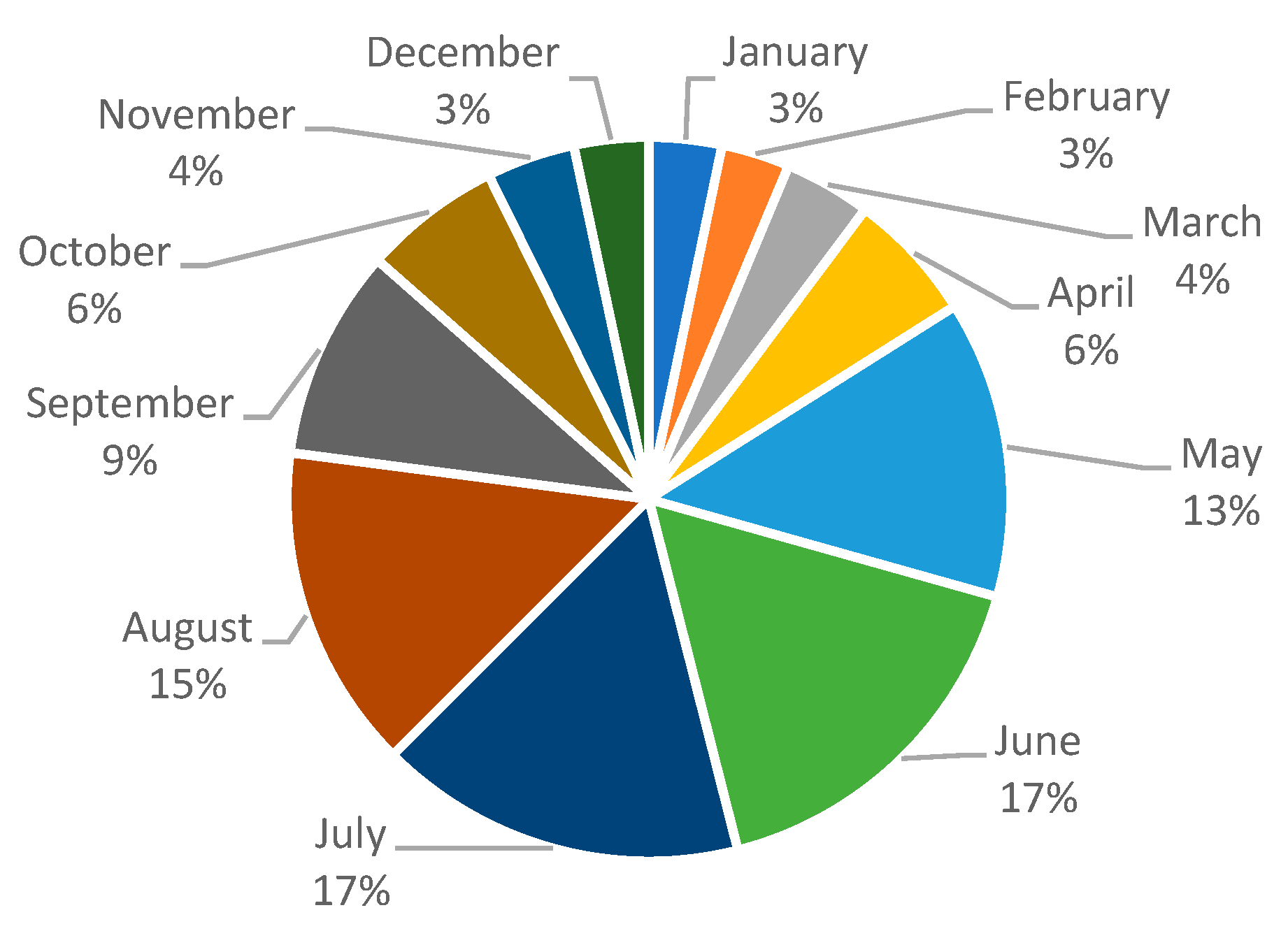
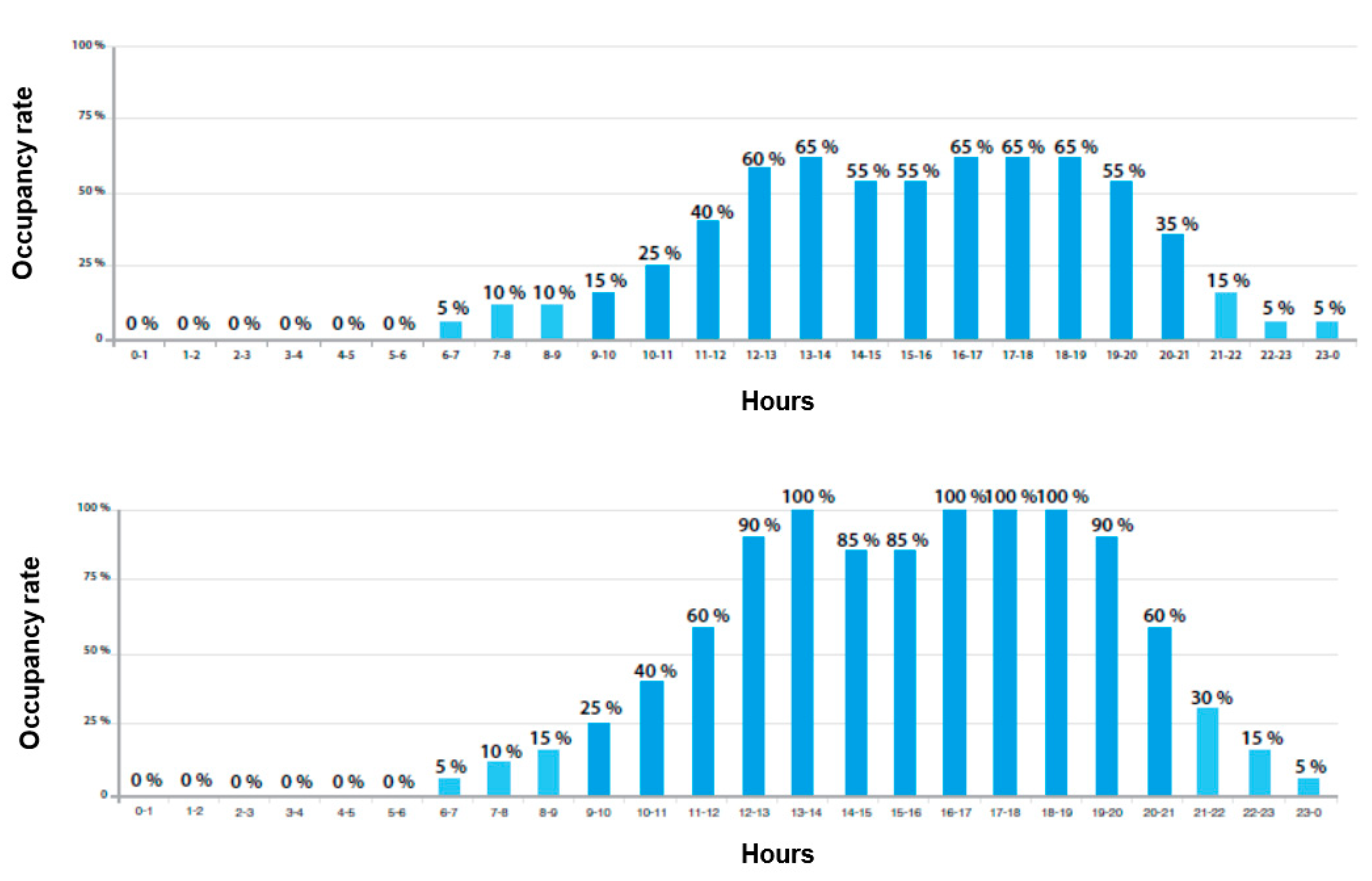
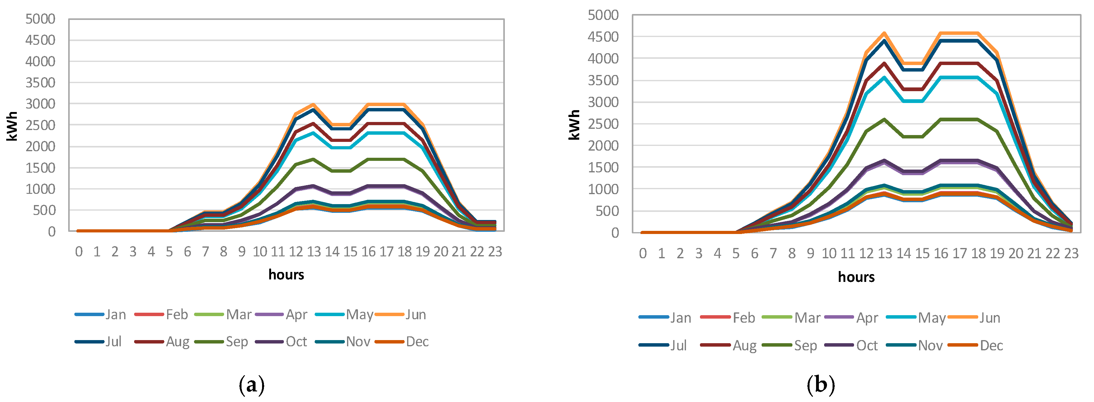
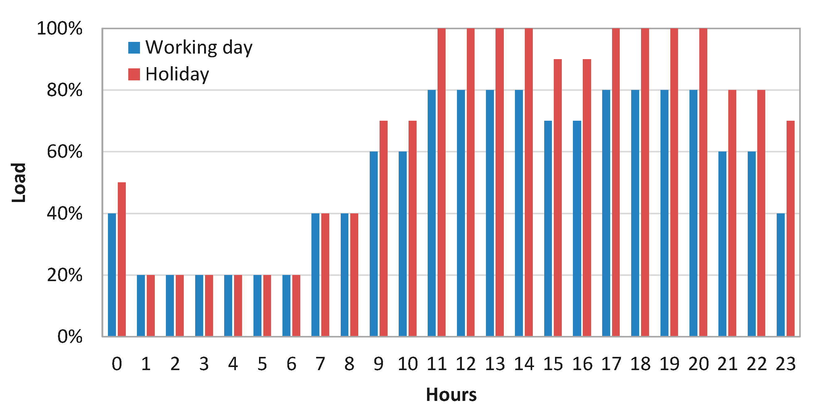
2. Energy Demands of the Commercial Centre

The proposed energy systems must attend to the electricity and cooling demands of a commercial center located in Zaragoza, Spain. Cooling is required for air conditioning throughout the year, even during winter months, to maintain comfortable indoor temperature conditions. The annual thermal cooling demand amounts to 6412 MWh_t and is satisfied by chilled water from 7 to 12 °C, produced by electricity-driven vapor compression refrigeration chillers. The annual thermal cooling demand is distributed throughout the year, considering the monthly thermal cooling demand data simulated for a similar consumer center and the hourly occupation rates on working days and holidays [51]. The monthly distribution of thermal cooling is shown in Figure 1. The occupancy of the consumer center is 18 h per day, corresponding to 12 h where it is open to the public (from hours 09 to 21) plus 6 h for services and supply (from hours 06 to 09 and 21 to 00). The occupancy profiles for working days and holidays are shown in Figure 2.

The hourly thermal cooling demand throughout the year is shown in Figure 3 for working days and holidays. Thermal cooling loads are notably higher on holidays, when the maximum occupancy is reached, than on working days. Moreover, they are significantly higher in the summer than in the winter months.

The annual electrical demand required for lighting, services, etc. (excluding the electricity consumption for chilled water production in the vapor compression refrigeration chillers) amounts to 1370 MWh_e. The daily electricity demands on a working day and on a holiday are 3465 kWh_e and 4264 kWh_e, respectively, and are the same throughout the year. The hourly distributions for each type of day are estimated according to the load profiles shown in Figure 4.

3. Description of the Analyzed Systems

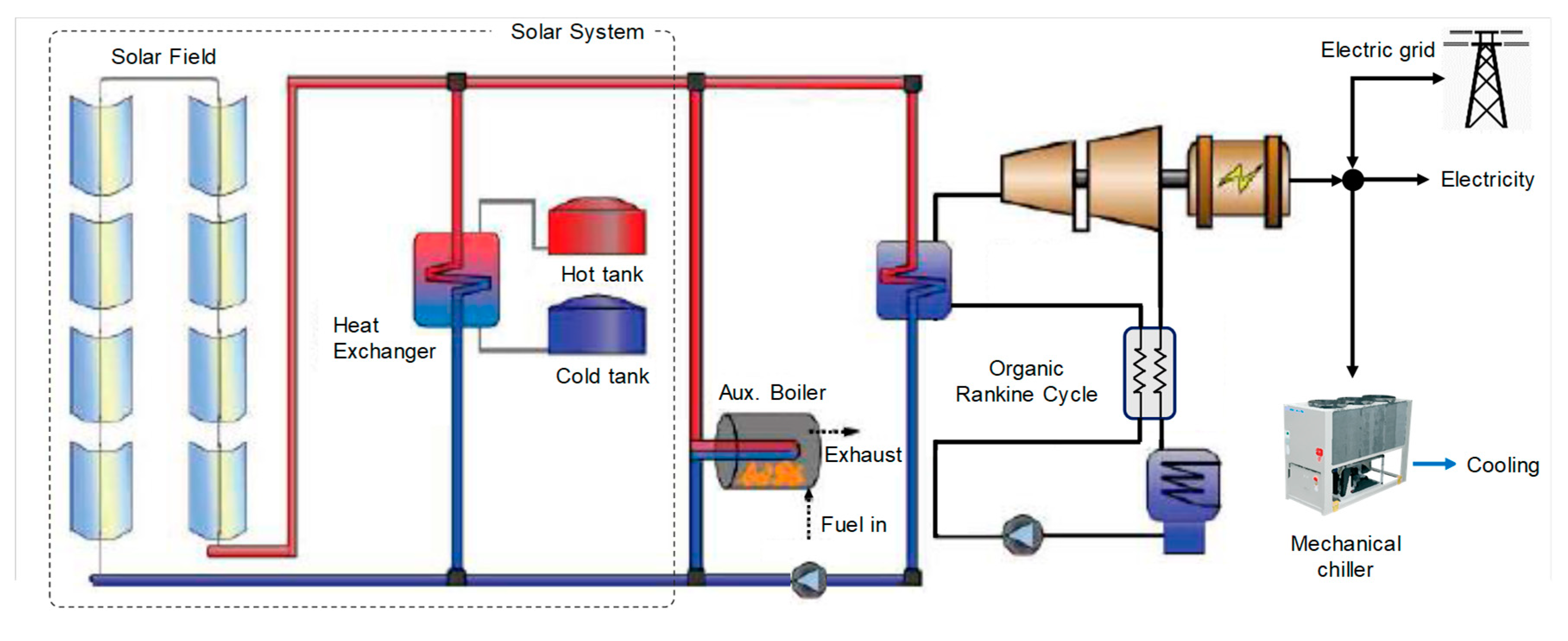
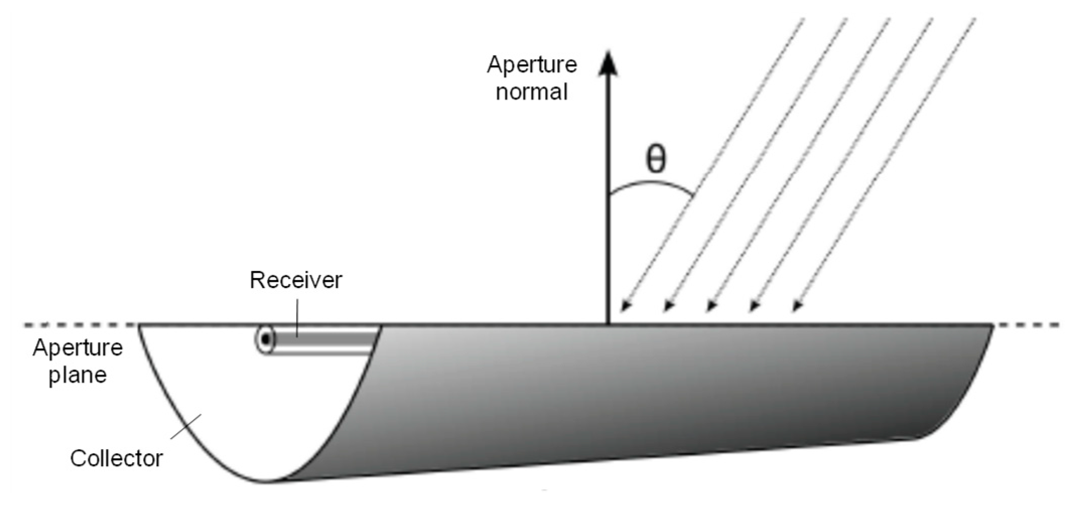
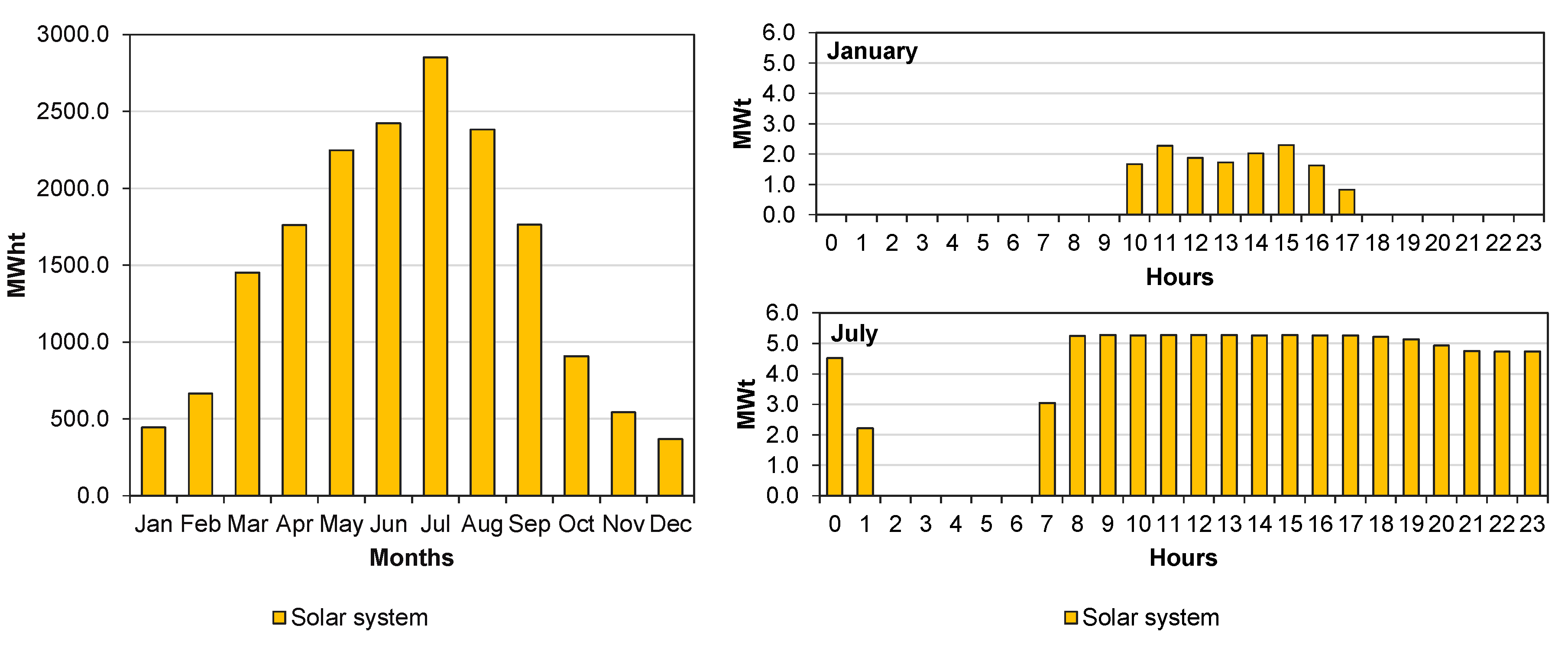
A simplified diagram of the solar-based cogeneration systems analyzed herein is depicted in Figure 5. System A consists of a solar system, composed of a solar parabolic trough collector field with thermal energy storage, integrated with an ORC and hybridized with a biomass boiler. It is assumed that the ORC only operates at full load and the biomass boiler complements the thermal output of the solar system whenever the solar resources are low, guaranteeing a constant thermal energy supply to the ORC, both in quantity and temperature. The system is in operation whenever there are enough solar resources available to operate the ORC, that is, the biomass boiler only operates during the operating hours of the solar system. In contrast, system B consists of a solar system integrated with an ORC without the biomass boiler hybridization. In this case, the ORC is exclusively driven by solar thermal energy and is allowed to operate at partial load whenever the solar resources are not enough to allow for full load operation.

Solar radiation, more specifically solar Direct Normal Irradiation (DNI), is harnessed by the parabolic trough collector field and transferred to the heat transfer fluid (HTF) as thermal energy. The solar collector field is connected to a TES in order to prolong the operation time and reduce the production variability, partially mitigating the non-simultaneity between the time period of solar resource availability and consumption. The assembly is connected to a heat exchanger (the ORC evaporator) where the thermal energy of the HTF is transferred to the ORC’s working fluid, allowing for the conversion of thermal energy into mechanical energy in the ORC. An alternator directly connected to the ORC turbine shaft transforms the mechanical energy into electricity, which is used to cover the electricity demand required for lighting and services, and to drive the vapor compression refrigeration chillers that produce the low-temperature thermal energy required for the cooling demand. The system is connected to the electrical grid, which allows electricity purchase when the demand exceeds the production, and electricity sale when there is an excess of electricity production. Thus, purchasing electricity from the grid ensures an appropriate electricity supply, and selling electricity to the grid generates revenue to improve the economic return of the investment.

Both systems A and B have been sized so that the annual electrical energy production is similar to that of a conventional system that covers the energy services with electricity purchased from the grid. The procedure for sizing the plant components of both systems is explained in detail in previous works developed by the authors [53,54]. The first step was the selection of the vapor compression refrigeration chillers that must cover the thermal cooling demands of the commercial center. In this way, the total annual electrical demand of the commercial center (electricity required for cooling and for other services) was determined. With this information, the ORCs for systems A and B that should produce the annual electricity consumed by the commercial center were selected and the heat input required by each ORC was thus determined. This information was used to size and design both solar systems, as well as, in the case of system A, the auxiliary biomass boiler, which complements the solar field’s thermal energy production in order to guarantee a constant thermal energy supply to the ORC. The appropriate sizing of the solar field area and TES capacity was determined for each system in order to minimize heat loss and maximize the solar thermal energy production with the quality (temperature level) required by each ORC. An iterative procedure was applied to properly match the thermal energy produced in each solar system and the heat input required by each ORC. The solar systems were assumed to be installed in an area next to the consumer center. The available surface area was sufficiently large so that it did not constitute an active restriction to the problem.

The technical data of the plant components selected are shown in Table 1. The following subsections describe the different plant components and explain the physical model developed to design and study the behavior and performance of both systems A and B throughout the year.

3.1. Solar System

The solar system was modelled and simulated using the System Advisor Model (SAM) [49], which is an open-source model oriented towards the feasibility assessment of renewable energy projects. A brief description of the mathematical model used for the simulation of the solar system is presented in the following paragraphs. The SAM simulation engine, integrated with TRNSYS [55], provides, among other things, a detailed hourly simulation performance of concentrating parabolic trough solar collectors, piping and thermal energy storage based on the physical principles of thermodynamics and heat transfer, considering transient effects related to variable solar radiation during the day and throughout the year, the thermal capacity of the HTF in the field piping, the headers, and the balance of the whole system [56].

Table 1. Solar-based cogeneration systems. Technical data of components.

Components		System A	System B
Solar System [49]	Total aperture reflective area	13,080 m2	19,620 m2
	Land area	32,375 m2	52,610 m2
	Field thermal output power	9.20 MWt	13.79 MWt
	Solar thermal energy produced	10,358 MWh/year	17,930 MWh/year
	Solar Collector
	Model	Siemens SunField 6	Siemens SunField 6
	Orientation	North-South	North-South
	Tilt	0°	0°
	Solar receiver
	Model	Siemens UVAC 2010	Siemens UVAC 2010
	Heat Transfer Fluid	Therminol 66	Therminol 66
	Tsf,out–Tsf,in of receiver HTF	214–121 °C	214–121 °C
	Thermal energy storage (TES)
	Thermal energy capacity	16.7 MWh	32.6 MWh
	Tank volume	356 m3	696 m3
	Hours of storage	6 h	6 h
Biomass boiler [57]	Thermal power	2.8 MWt	-
	Energy efficiency (LHV basis)	0.82	-
	Biomass LHV	15.5 MJ/kg	-
Mechanical chillers [58]	Model	Cobalt W 153.3	Cobalt W 153.3
	Number of chillers	3	3
	Refrigerant	R134a	R134a
	Nominal cooling capacity per chiller	1527 kWt	1527 kWt
	Nominal electrical input power	326 kWe	326 kWe
	EER (nominal)	4.68	4.68
	Water temperature at condenser (in–out)	30–35 °C	30–35 °C
	Water temperature at evaporator (in–out)	12–7 °C	12–7 °C
Organic Rankine Cycle (ORC) [50]	Type	Single pressure with regenerative preheating	Single pressure with regenerative preheating
	Number of ORCs	1	1
	Electric efficiency (full load)	0.18	0.18
	Nominal electrical power	500 kWe	978 kWe
	Thermal input power	2.78 MWt	5.43 MWt

Table 1. Solar-based cogeneration systems. Technical data of components.

Components		System A	System B
Solar System [49]	Total aperture reflective area	13,080 m2	19,620 m2
	Land area	32,375 m2	52,610 m2
	Field thermal output power	9.20 MWt	13.79 MWt
	Solar thermal energy produced	10,358 MWh/year	17,930 MWh/year
	Solar Collector
	Model	Siemens SunField 6	Siemens SunField 6
	Orientation	North-South	North-South
	Tilt	0°	0°
	Solar receiver
	Model	Siemens UVAC 2010	Siemens UVAC 2010
	Heat Transfer Fluid	Therminol 66	Therminol 66
	Tsf,out–Tsf,in of receiver HTF	214–121 °C	214–121 °C
	Thermal energy storage (TES)
	Thermal energy capacity	16.7 MWh	32.6 MWh
	Tank volume	356 m3	696 m3
	Hours of storage	6 h	6 h
Biomass boiler [57]	Thermal power	2.8 MWt	-
	Energy efficiency (LHV basis)	0.82	-
	Biomass LHV	15.5 MJ/kg	-
Mechanical chillers [58]	Model	Cobalt W 153.3	Cobalt W 153.3
	Number of chillers	3	3
	Refrigerant	R134a	R134a
	Nominal cooling capacity per chiller	1527 kWt	1527 kWt
	Nominal electrical input power	326 kWe	326 kWe
	EER (nominal)	4.68	4.68
	Water temperature at condenser (in–out)	30–35 °C	30–35 °C
	Water temperature at evaporator (in–out)	12–7 °C	12–7 °C
Organic Rankine Cycle (ORC) [50]	Type	Single pressure with regenerative preheating	Single pressure with regenerative preheating
	Number of ORCs	1	1
	Electric efficiency (full load)	0.18	0.18
	Nominal electrical power	500 kWe	978 kWe
	Thermal input power	2.78 MWt	5.43 MWt

The solar field consists of solar collector assemblies (SCA) that are combined in one or more parallel loops (Figure 5). Each SCA is composed of a parabolic collector and its receiver, as depicted in Figure 6. SCAs are connected in series in each loop in order to incrementally increase the HTF temperature to the designed outlet loop HTF temperature value. In this model, the SCA serves as the lowest level of discretization and they are considered as a single unit when calculating the model. Thus, the absorbed energy, losses, temperature, pressure drop, and other performance values are calculated independently for each SCA [49,56].

The energy balance of a control volume encompassing the HTF within the absorber tubes and piping for a single SCA is

$$\frac{\partial U}{\partial t}={\dot{m}}_{htf}·c_{htf}·\left(T_{in}-T_{out}\right)+{\dot{q}}_{abs}$$

(1)

being

$$\frac{\partial U}{\partial t}=\left(m·c_{htf}+{\left(mc\right)}_{bal,sca}·L\right)\frac{\partial T}{\partial t}$$

(2)

where the internal energy, U, term represents the change of energy of the control volume with time, m is the mass of the HTF in the control volume of the SCA, c_htf is the specific heat of the HTF, L is the length of a single SCA, (mc)_bal,sca is the thermal capacitance per unit of length of joints, piping, insulation and other SCA pieces of equipment that also experience thermal inertia effects, T_in and T_out are the inlet and outlet temperatures of the HTF to each SCA, ${\dot{m}}_{htf}$ is the HTF mass flow rate, which is constant across the boundary of the SCA and ${\dot{q}}_{abs}$ is the rate of absorbed solar thermal energy in the receiver.

By applying the previous energy balance, which is a first order differential equation, successively to each SCA, all the temperature values of the HTF in the solar field are obtained, considering that the HTF inlet temperature to each SCA is the outlet temperature of the previous SCA. In order to meet the design value of the outlet loop HTF temperature, the mass flow rate of the HTF is varied. If the calculated HTF mass flow rate in the loop is lower than the minimum accepted value, then the software resets the mass flow rate to the minimum allowable and the outlet loop HTF temperature will be lower than the design value. When the solar field absorbs more energy than required to reach the design value of the outlet loop HTF temperature, even with the maximum HTF mass flow rate accepted value, the system controller defocuses some collectors in order to reduce the harnessed solar energy and to avoid overheating the HTF [52,56].

The collector model determines the magnitude of incident solar flux on the receiver, considering constant and variable optical losses. Constant optical losses encompass tracking errors, imperfections in the collector geometry, reflectance and soiling of the mirrors. Variable optical losses depend on the solar position. The most important variable losses are the so-called cosine losses, proportional to the cosine of the incidence angle θ of the solar irradiation, which is the angle between the solar irradiation and the normal to the aperture plane, as shown in Figure 6. Other position losses considered are losses of reflected radiation at the end of the collector row (spillage losses), shadowing caused by other collector rows, available solar energy not being harnessed early in the morning and late in the evening, and an incident angle modifier accounting for the remaining variable optical losses [52,56].

The receiver is modelled as a one-dimensional energy flow, following the model developed by Forristall [59]. Only temperature gradient in the radial direction is considered significant. Figure 7a presents a diagram of a quarter of a cross section of the receiver. Temperatures T₁ to T₅ are calculated by applying thermal energy balance and a thermal resistance heat transfer model (Figure 7b). The geometry of the receiver is specified as well as the glass envelope absorptance and transmittance. Concentrated solar irradiation flux passes through the glass envelope, where a small fraction is absorbed, and unabsorbed irradiation reaches the absorber tube. Thermal energy is transferred through the absorption tube wall to the HTF. Thermal losses occur in the absorber tube and glass envelope surfaces due to convection and radiation mechanisms [52,56].

The SAM model also calculates the pressure drop occurring in several field components, e.g., piping from and to the solar field headers, receiver tube piping, elbows and valves. The total HTF volume and surface area of the piping are considered, with the exception of the surface area of the receiver absorber. The model applies a specific heat loss coefficient to the piping surface area, which depends on its temperature, to calculate the thermal energy loss from pipes [52,56].

As shown in Figure 5, we also consider the integration of TES into the system, in order to increase the stability of the solar field production. Both cold and hot tanks are designed to store the entire HTF volume. The tanks are assumed to be fully thermally mixed without stratification. The capacity of the tank is expressed in equivalent hours of the solar system operation at full load, that is, the number of hours that the storage system can supply energy at a design point. In terms of thermal energy, the total TES thermal capacity, E_tes, is equal to the design point thermal requirement that the solar system should provide times the total number of desired storage hours. The volume of HTF, V_tes, required to match the TES energy content is calculated by Equation (3), considering average material properties for the hot and cold tank design temperatures [52,56].

$$V_{tes}=\frac{E_{tes}}{{\rho }_{tes,ave}·c_{tes,ave}·f_{hx}·\left(T_{sf,out}-T_{sf,in}\right)}$$

(3)

where ρ_tes,ave and c_tes,ave are, respectively, the average density and specific heat of the HTF, and the design temperature difference is equal to the hot solar field outlet temperature T_sf,out minus the cold solar field return temperature T_sf,in multiplied by the heat exchanger factor f_hx, which is the ratio of the temperature difference on the TES side of the heat exchanger to the solar field side temperature difference. The hot and cold tanks are modelled separately using the variable tank model (type 39) in TRNSYS [55]. The heat exchanger connecting the solar field and the TES (see Figure 5) is modelled with the effectiveness-NTU method, considering the counterflow arrangement. SAM calculates the size of the heat exchanger from the solar system design values [52,56].

The input parameters for the simulation of the solar systems with SAM are described as follows. For both systems A and B, the solar collector model Siemens SunField 6 and the receiver Siemens UVAC 2010 were selected. All required data about geometry, materials and required technical specifications are available in SAM’s libraries [49]. The selected HTF that flows through the receiver tube is Therminol 66. It is able to cover an extended operating range, from −85 °C to 400 °C, and its common applications are heating and cooling processes, exploiting the fluid as a thermal vector for transporting energy [60]. The solar field outlet temperature T_sf,out and solar field return temperature T_sf,in values, as well as the thermal power provided by the solar system, were selected in an appropriate range to operate the selected ORCs. The chosen collectors’ orientation was the north–south direction, which collects more energy in summer than in winter. This alternative has been considered as the best choice because the application of this system aims to cover the cooling demand, which is higher in summer. In order to design the collector parabolic field, the model uses the design point at the DNI value (950 W/m²) with the sun position at noon on the summer solstice (21 June north of the equator, and 21 December south of the equator). Weather conditions at the plant location (Zaragoza, Spain) were taken from the Meteonorm database [61].

The appropriate match between the solar field area and the TES capacity was also taken into account. By keeping the TES capacity constant, increasing the solar field area enabled a higher annual solar thermal energy production, but this effect was gradually reduced because, with an oversized solar field, a greater amount of harnessed solar energy could not be stored and was not used. Furthermore, for the same solar field area, increasing the TES capacity promoted a rise in the annual solar thermal energy production, but when the TES capacity was oversized the increase in the solar thermal production was reduced. A more detailed analysis is provided in [53,54].

3.2. Biomass Boiler

The hybridization of the solar system with a biomass boiler is only considered in the case of system A. The biomass boiler complements the solar field production whenever the solar resources are not able to supply the thermal power required by the ORC to run at full load, thus allowing for a more stable operation of the power production system. Therefore, the use of the biomass boiler, which is installed in parallel with the solar system, as shown in Figure 5, is only allowed during the operating hours of the solar system. The considered biomass boiler is a moving grate furnace with a nominal thermal power of 2.8 MW_t and energy efficiency (LHV basis) of 0.82, fed with commercial biomass pellets [57].

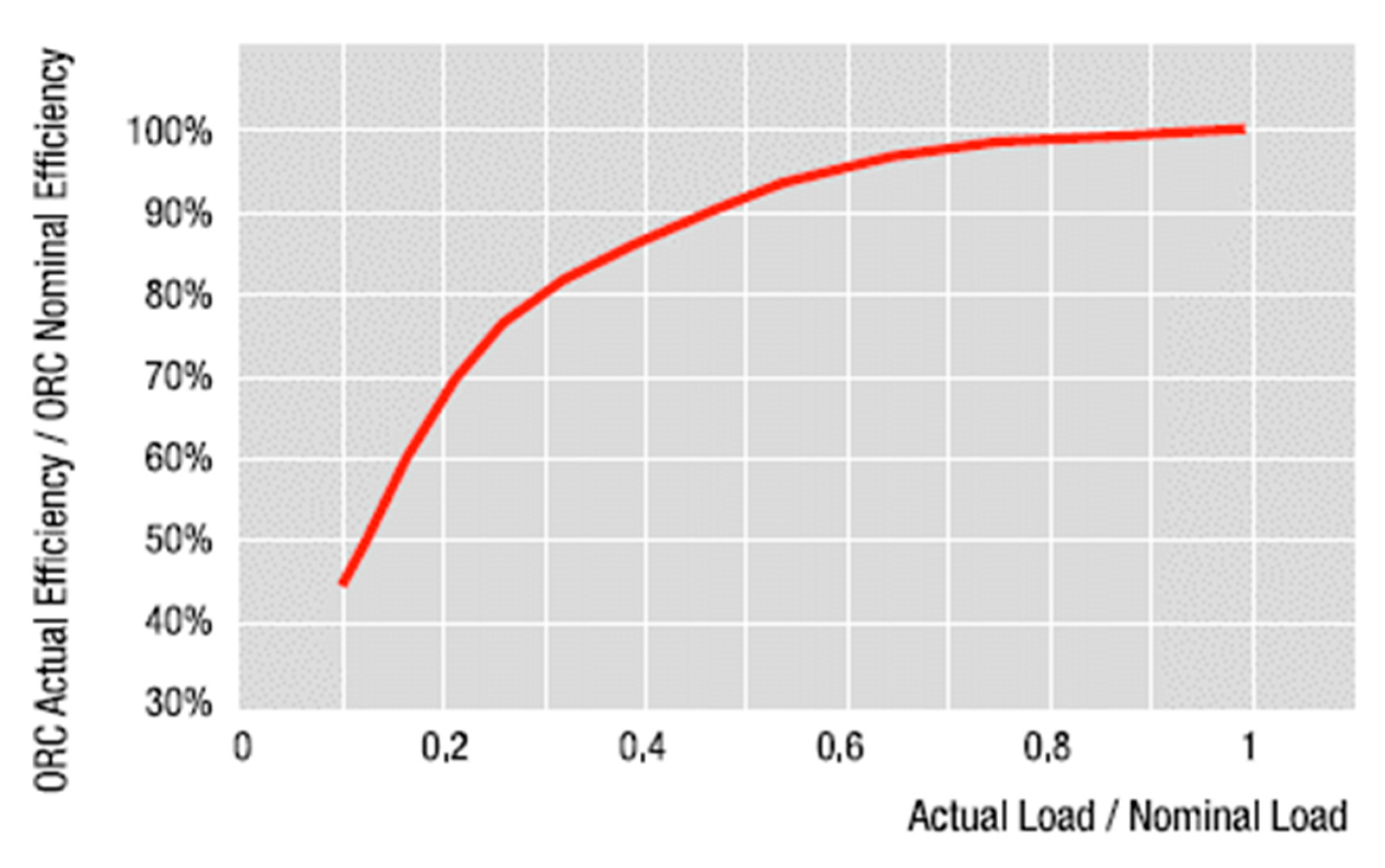
3.3. Organic Rankine Cycle

The purpose of the ORC is to produce electricity from the heat supplied by the solar system hybridized with the biomass boiler, in the case of system A, and by the solar system alone, in the case of system B. Covering the annual electricity consumption of the commercial center was the design criterion of both systems. Therefore, following the procedure described in [53,54], and considering the technical features and data of Turboden 6/7 HR and Turboden 10/14 HR [50], the selected ORCs were: (i) 500 kW_e of nominal electrical power, with a nominal energy efficiency of 18% in the case of system A, in which the ORC only operates at full load; and (ii) 978 kW_e of nominal electrical power, with the same nominal energy efficiency of 18% in the case of system B, in which the ORC is allowed to operate at partial load. As a result, the thermal power input required by each ORC at full load operation corresponds to 2.78 MW_t and 5.43 MW_t for systems A and B, respectively. The inlet and outlet temperatures of the HTF that feeds each ORC are 214 °C and 121 °C (Table 1), respectively. These temperature values are in agreement with the technical data of selected ORCs [50].

The selected ORCs are single-pressure cycles with regenerative preheating of the organic fluid [50]. The appropriate integration of each ORC with the heat source in all the analyzed cases was verified through a thermodynamic model of the Rankine Cycle, built with the Engineering Equation Solver (EES) software [62], considering R245fa as the working fluid due to its favorable behavior [63]. Taking into account the technical characteristics and operating conditions of the ORCs considered herein, the thermodynamic cycles were replicated, assuming reasonable values for the technical performance parameters (e.g., isentropic efficiencies in turbine, pump, regenerative heat exchanger effectiveness, minimum temperature differences in evaporator and condenser) of the different pieces of equipment of the ORCs [28]. The results were in agreement with commercial equipment and performance data provided by Turboden [50]. Based on Turboden technical data, the ORC can provide part-load operation down to 10% of nominal load and maintain 90% of the cycle efficiency down to a 50% load, as shown in Figure 8. It was confirmed that, even at the partial load operation of the ORC integrated with the solar system in the case of system B, fundamental physical laws, particularly the Second Law of thermodynamics, were fulfilled.

3.4. Mechanical Chiller

Vapor compression refrigeration chillers (mechanical chillers), based on a reverse Rankine Cycle, cover the annual thermal cooling demand (6455 MWh_t) of the considered commercial center, consuming electricity produced by the ORC and/or electricity purchased from the electric grid, and producing chilled water at 7 °C. The commercial chiller selected was COBALT W 153.3 [58], whose technical data are shown in Table 1. Monthly and daily electrical demand profiles for cooling throughout the year have been evaluated and their shapes are similar to the thermal cooling demand profiles shown in Figure 3, but corrected with the chiller’s Energy Efficiency of Refrigeration (EER = 4.68). In order to guarantee the cooling demand, three mechanical chillers were considered to be installed in both systems A and B, with a total nominal cooling thermal power capacity of 4581 kW_t and 978 kW_e nominal electrical power.

4. Operation of the Analyzed Systems

This section describes the annual, monthly, and hourly operation of systems A and B. It is worth keeping in mind the following: (i) there is a cooling demand for air conditioning throughout the year (see Figure 1 and Figure 3); (ii) the ORC is in operation only during the operating hours of the solar system—for the rest of the time, the electricity required must be purchased from the grid; (iii) in system A, the ORC is operating at full load with the support of the biomass boiler, which complements the thermal power produced by the solar system; (iv) in system B, there is not an auxiliary biomass boiler and the ORC can modulate operating at partial load according to the thermal power supplied by the solar system; and (v) electricity purchase and sale are allowed when there is deficit or excess of production, respectively.

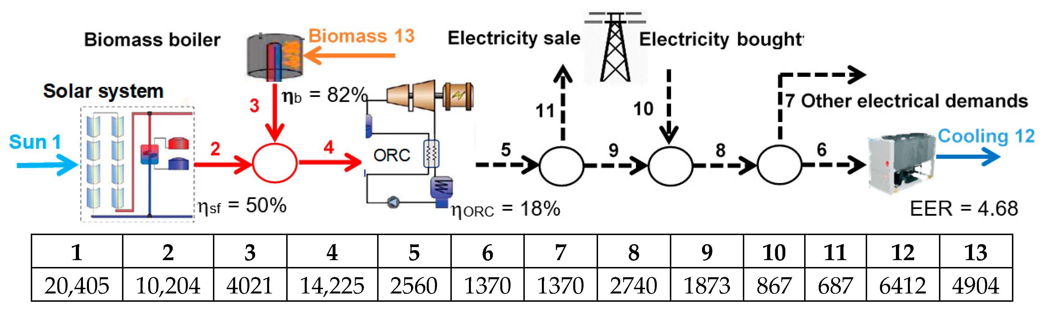
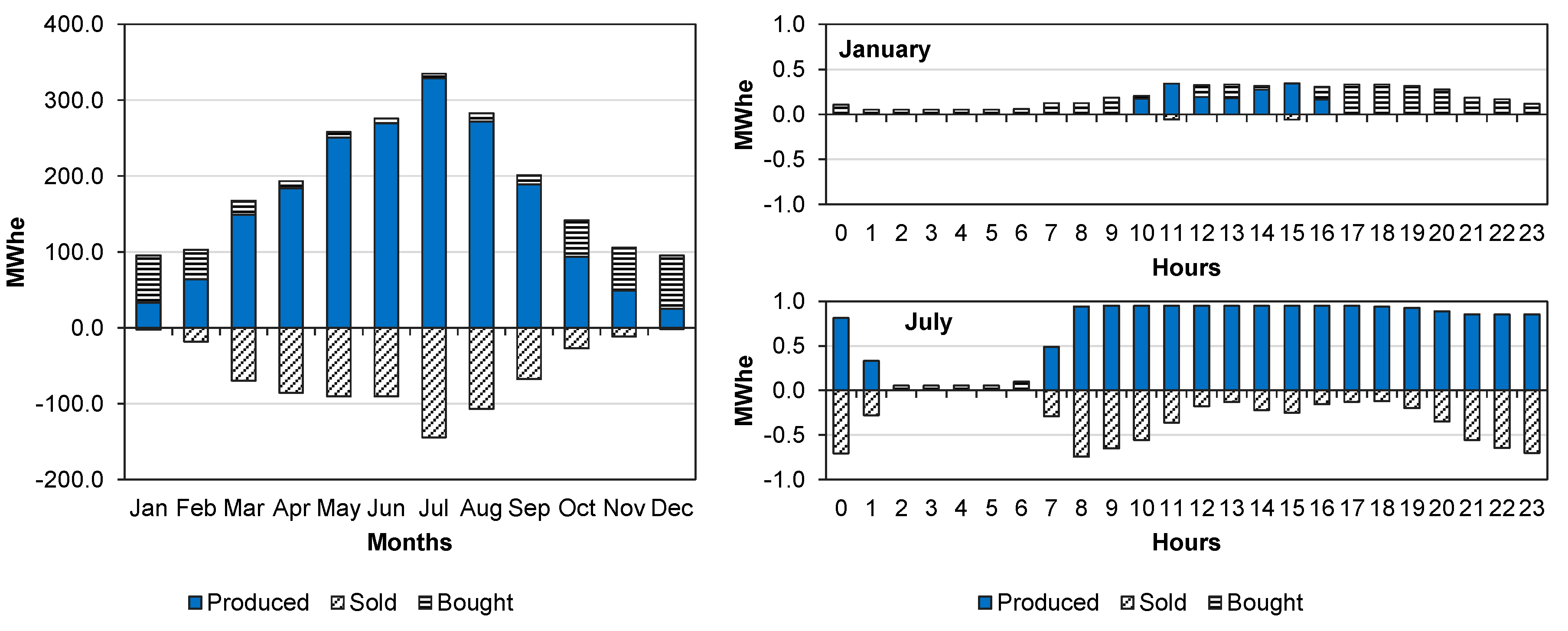
4.1. System A: Hybrid Solar Parabolic Trough–ORC–Biomass System

It has been considered that system A starts its operation when the harnessed solar power is higher than 0.5 MW_t. Therefore, the total annual hours of operation of the system reach 5117 h/year. The annual energy balance of the whole system is shown in Figure 9.

On an annual basis, the solar system (#2) produces 72% of the thermal energy (#4) and electrical energy (#5) of the cogeneration plant, while the biomass boiler contributes the remaining 28% (#3). The total electricity produced by the ORC (#5) amounts to 2560 MWh_e. This would be enough to cover almost all (93%) of the electrical requirements (#8) for cooling (#6) and for electricity demands (#7). However, due to the irregular availability of solar resources, even with the support of the thermal energy storage and the biomass boiler, only 73% of the electricity produced (#5) is actually consumed by the system (#9), while the remaining 27% is sold to the grid (#11), and the system must purchase 867 MWh_e of electricity from the grid (#10). The obtained renewable (solar + biomass) and solar fractions in the electricity consumed by the system (#8) are about 68% (#9/#8) and 49% (#2/#4·#9/#8), respectively. Noteworthily, the electricity required for cooling (#6) is virtually the same as the electricity demand of the commercial center (#7).

Table 2. Monthly energy balance of the hybrid solar parabolic trough–ORC–biomass plant (system A), MWh/month.

Flow	Jan	Feb	Mar	Apr	May	Jun	Jul	Aug	Sep	Oct	Nov	Dec
1	651	847	1630	1943	2493	2666	3200	2567	1955	1117	767	567
2	280	423	863	1011	1272	1314	1519	1331	1019	596	352	226
3	410	356	430	407	366	271	119	134	399	438	315	377
4	689	778	1292	1417	1637	1584	1637	1465	1417	1034	667	603
5	124	140	232	255	294	285	294	263	255	186	120	109
6	44	42	53	80	182	229	225	199	129	85	54	46
7	116	105	116	113	116	113	116	116	113	116	113	116
8	161	147	169	193	299	341	342	315	242	201	167	162
9	83	97	147	171	217	216	222	212	194	151	88	72
10	78	50	22	21	82	125	119	104	48	50	79	90
11	41	43	85	84	78	69	72	52	61	35	32	36
12	208	196	249	374	854	1070	1055	932	606	397	254	214
13	500	434	524	496	446	331	145	164	486	535	385	460

shows the monthly energy balance of system A. Due to the higher availability of solar resources in the summer, with more direct sunlight hours than in the winter: (i) the contribution of the solar system (#2) increases in the summer, reaching about 93% of the thermal production (#4) in July, compared to only 37% in December; (ii) the solar system operates for more hours in the summer, so that electricity production in the ORC also increases, being almost three times higher in July than in December. These effects are explained further for the hourly operation of the system.

The dynamic hourly behavior throughout the year of the solar system (solar field integrated with TES) is obtained with SAM [49]. Figure 10 shows the hourly profiles on a typical day in selected months of the year: (i) the total incident thermal power (MW_t) to the solar field considering the deviation with respect to the normal solar irradiance; (ii) the thermal power (MW_t) harnessed by the HTF in the receiver; (iii) the thermal power (MW_t) released to the ORC (heat sink); (iv) the thermal power (MW_t) discharged from the TES; and (v) the thermal power (MW_t) charged to the TES. Note that hourly values of these magnitudes for the whole year have been calculated, obtaining detailed information about the hourly available solar resources and the hourly solar thermal energy released to the ORC, as well as detailed information about each piece of equipment in the solar system, including the hourly behavior of the TES throughout the year.

The monthly thermal energy provided by the solar system and biomass boiler is shown on the left side of Figure 11. On the right side are the hourly thermal productions during a day in January (winter) and a day in July (summer). As previously explained, the operation of the solar system starts after the thermal output reaches the threshold of 0.5 MW_t, so that the operating hours of the solar system vary significantly throughout the year according to the solar resource availability, as in January (8 h/day) and in July (19 h/day). Moreover, since the biomass boiler only works during the operating hours of the solar system, to complement the thermal output necessary to reach the ORC’s required thermal input nominal power: (i) the sum of the solar and biomass thermal energy in each hour is always equal to 2.78 MW_t; and (ii) the hourly contribution of the biomass boiler is higher in the winter months, when there are less available solar resources, as in January the biomass boiler covers about 60% of the daily thermal production, with a well-distributed load throughout the day, while in July it covers only 7%, being much more prominent at hours 01 and 07.

While the thermal energy production of the solar system and biomass boiler is the same on each day of the month, the electricity requirements (electricity demand and electricity for cooling demands) of the commercial center presented two different profiles, namely working days and holidays, as explained in Section 2. Figure 12 shows the distribution of the electricity produced by the ORC, bought from and sold to the electric grid on working days; on the left side, the monthly distribution is shown and on the right side the hourly values for January (winter) and July (summer) are shown. As can be seen, electricity production in the ORC follows the thermal energy availability, being higher in the summer months and lower in winter. Regarding the hourly profiles, for a working day in January, the system generates surplus electricity, which is sold to the grid from hours 10 to 17, and there is no need for electricity purchase (during operating hours of the solar system). On the other hand, for a working day in July, the high electricity requirements lead the system to purchase electricity from hours 11 to 20.

Similarly, Figure 13 presents the monthly and hourly distributions of the electricity produced by the ORC, bought from and sold to the electric grid on holidays by system A. It should be noted that the monthly values shown in Figure 13 are lower than the ones shown in Figure 12 because the number of holidays per month is about half of the number of working days. In fact, as explained in Section 2, taken individually, holidays presented higher electricity requirements (electricity demand and electricity for cooling demand) than working days. On a holiday in January (winter), while the system is in operation, it is not necessary to purchase electricity from the grid, and even a small part of the electricity produced is sold. However, on a holiday in July (summer), the higher electricity requirements lead the system to purchase electricity from the grid from hours 10 to 20, limiting the electricity sale.

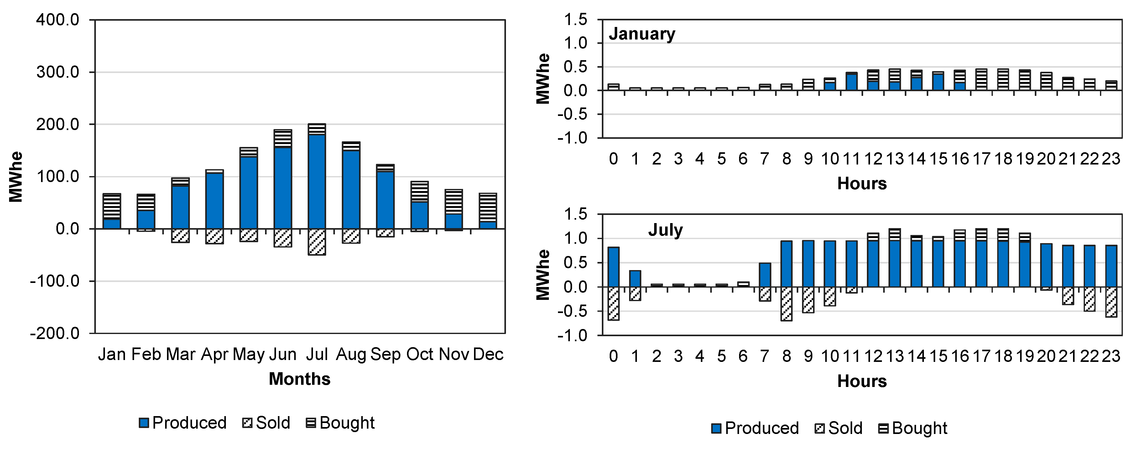
4.2. System B: Parabolic Trough–ORC System

In the previous section, the ORC of the proposed hybridized system was always operating at full load (500 kW_e), thanks to the support of the biomass auxiliary boiler, which complemented the thermal power produced during the operating hours of the solar collectors. This section analyzes the behavior of the cogeneration plant without the support of the biomass boiler and allowing partial load operation of the ORC, according to the technical data of the manufacturer of the selected ORC shown in Figure 8 [50]. A simplified diagram of system B is shown in Figure 14. The main components (i.e., solar system and ORC) have been resized following the procedure explained in [53,54] to fulfil the criterion of supplying a similar amount of annual electrical energy to that of a conventional system based on electricity purchased from the grid of the commercial center. The technical specifications of system B are shown in Table 1.

The annual energy balance of system B for a year of operation is shown in Figure 14. In this case, the solar system produces 2979 MWh_e (#5), which is slightly higher than the annual electrical demand, 2740 MWh_e (#8), of the commercial center for cooling (#6) and for other electrical demands (#7). However, due to the irregular availability of solar resources, even with the support of thermal energy storage, only about 69% of the electricity produced by the ORC is actually consumed (#9), while the remaining 31% is sold to the electric grid (#11), and the system is required to purchase 690 MWh_e from the electric grid (#10). The resulting solar fraction in the electricity consumed by the system (#8) is thus approximately 75% (#9/#8).

Table 3. Monthly energy balance of the solar parabolic trough–ORC analyzed plant (system B), MWh/month.

Flow	Jan	Feb	Mar	Apr	May	Jun	Jul	Aug	Sep	Oct	Nov	Dec
1	842	1095	2109	2514	3225	3449	4140	3321	2529	1445	992	733
2	443	665	1453	1761	2246	2422	2851	2382	1763	908	542	368
5	52	100	231	291	389	425	509	421	299	145	78	39
6	44	42	53	80	182	229	225	199	129	85	54	46
7	116	105	116	113	116	113	116	116	113	116	113	116
8	161	147	169	193	299	341	342	315	242	201	167	162
9	49	77	136	177	274	300	315	288	217	114	64	38
10	111	70	34	15	25	41	26	28	25	87	103	124
11	2	22	95	114	115	125	194	134	82	32	14	1
12	208	196	249	374	854	1070	1055	932	606	397	254	214

shows the monthly energy balance of system B. This shows how the solar system is able to produce (#5) the electricity required for cooling (#6) during all the months of the year, except in December, and is able to produce more electricity (#5) than demanded (#8) for seven months, from March to September. Nevertheless, it should be noted that even in summer months, when the electricity production is higher because there is a higher availability of solar resources, it is also necessary to purchase electricity in order to fulfil the electrical demands of the commercial center during the night, e.g., in July, the electricity produced (#5) is close to 150% of the electricity demanded (#8), but the system must still purchase about 26 MWh_e from the grid (#10).

Table 4. Hourly values of thermal power (MW_t) provided by the solar system (#2) of the solar parabolic trough–ORC plant (system B).

Hour	Jan	Feb	Mar	Apr	May	Jun	Jul	Aug	Sep	Oct	Nov	Dec
00	0.00	0.00	0.00	1.17	2.06	3.50	4.52	2.36	0.00	0.00	0.00	0.00
01	0.00	0.00	0.00	0.00	0.74	1.76	2.21	0.00	0.00	0.00	0.00	0.00
02	0.00	0.00	0.00	0.00	0.00	0.00	0.00	0.00	0.00	0.00	0.00	0.00
03	0.00	0.00	0.00	0.00	0.00	0.00	0.00	0.00	0.00	0.00	0.00	0.00
04	0.00	0.00	0.00	0.00	0.00	0.00	0.00	0.00	0.00	0.00	0.00	0.00
05	0.00	0.00	0.00	0.00	0.00	0.00	0.00	0.00	0.00	0.00	0.00	0.00
06	0.00	0.00	0.00	0.00	0.00	0.00	0.00	0.00	0.00	0.00	0.00	0.00
07	0.00	0.00	0.00	0.00	2.54	3.31	3.04	0.00	0.00	0.00	0.00	0.00
08	0.00	0.00	0.52	3.55	4.35	4.64	5.24	4.39	2.43	0.00	0.00	0.00
09	0.00	0.00	3.58	4.17	4.48	4.90	5.28	4.94	4.16	2.41	0.00	0.00
10	1.67	2.28	4.22	4.25	4.70	4.95	5.27	4.95	4.23	3.26	2.60	1.33
11	2.27	2.50	4.00	4.18	4.68	4.87	5.27	5.05	4.27	3.21	2.54	1.73
12	1.87	2.58	3.92	4.21	4.70	4.85	5.27	5.11	4.34	3.24	2.25	1.41
13	1.73	2.55	3.77	4.27	4.80	4.88	5.28	5.13	4.55	3.42	2.18	1.33
14	2.02	3.00	4.12	4.36	4.57	4.81	5.26	5.12	4.43	3.47	2.67	1.85
15	2.30	3.18	4.04	4.20	4.54	4.79	5.27	5.10	4.57	3.51	3.39	2.41
16	1.62	3.57	3.93	4.05	4.47	4.68	5.27	5.14	4.63	3.33	1.53	1.06
17	0.82	2.33	3.83	3.78	4.49	4.55	5.27	5.16	4.24	2.19	0.89	0.73
18	0.00	1.22	3.00	3.47	4.47	4.56	5.21	5.03	3.74	1.25	0.00	0.00
19	0.00	0.54	2.47	3.24	4.36	4.37	5.14	4.95	3.43	0.00	0.00	0.00
20	0.00	0.00	1.91	2.90	3.96	4.04	4.93	4.18	2.99	0.00	0.00	0.00
21	0.00	0.00	1.58	2.60	3.11	3.86	4.75	3.63	2.70	0.00	0.00	0.00
22	0.00	0.00	1.23	2.40	2.80	3.80	4.73	3.38	2.19	0.00	0.00	0.00
23	0.00	0.00	0.75	1.90	2.63	3.62	4.74	3.21	1.86	0.00	0.00	0.00

shows the hourly values of thermal power provided by the solar system, obtained from the dynamic simulation of the solar system in SAM [49]. These values represent the inputted thermal energy of the ORC for the production of electricity. According to the partial load operation chart of the ORC shown in Figure 8, the minimum thermal input required for the operation of the ORC is about 1 MW_t and the maximum at full load is 5.43 MW_t. Therefore, the ORC could be in operation for about 4874 h per year. The nominal electrical efficiency value of the ORC at full load is 18% (see Table 1), and during the annual operation of system B, the annual average electrical efficiency of the ORC reaches 16.7% (Figure 14). According to Figure 8, the energy efficiency of the ORC remains at its maximum value (18%) for operating loads between 80% and 100%. That is, when the thermal input is higher than 4 MW_t, the energy efficiency of the ORC is maximum, and for a thermal input over 3 MW_t (50% load), the energy efficiency of the ORC is about 16%. The values presented in Table 4 show that the ORC was operating at loads higher than 50% for most of the year (8 months), being especially high in the summer months (May to September, higher than 80% and reaching full load most of the time), while falling below 50% in the winter (November to February).

The monthly values of thermal energy production of the solar system of system B are shown on the left side of Figure 15. As expected, in summer months, the thermal energy production is five times higher than in winter months, which is a wider variation than in the case of system A, supported with a biomass boiler. The hourly thermal productions of the hybrid system on a day in January and in July are shown on the right side of Figure 15. In January (winter), the system is in operation for 8 h/day, during which the thermal power provided to the ORC is always lower than 3 MW_t. This means that the ORC operates below a 50% load at all the operation times, even being at its technical limit of a 10% load at hour 17, which is an unfavorable operation condition in terms of the technical feasibility and reliability of the system. In July (summer), the system is in operation for 19 h/day, and its operation is close to 100% load for about 12 h. The rest of the time, the system is operating above an 80% load and modulates its operation between 30 and 50% loads at the times at which the system starts up and shuts down.

For system B, the monthly electricity produced, bought and sold is presented for working days in Figure 16 and for holidays in Figure 17. As can be seen, electricity purchases on working days are more restricted to colder months (from October to February), being particularly low during the rest of the year, when electricity sale is more pronounced. On the other hand, on holidays the system must purchase electricity all year round, except for the months of March and April, when it is able to sell relatively less electricity to the grid. As explained for system A, it should be noted that the monthly values shown in Figure 17 are lower than the ones shown in Figure 16 because the number of holidays per month is about half of the number of working days.

The hourly electricity produced, bought from and sold to the electric grid on working days and holidays in January (winter) and July (summer) is shown on the right side of Figure 16 and Figure 17. It is shown that, on a working day in January, the system is able to cover virtually all of the electricity requirements of the commercial center for almost 4 h, with it even being possible to sell a very reduced quantity of electricity at hours 11 and 15. In contrast, on a holiday in January, the system only reaches electricity self-sufficiency for about 2 h, and no electricity sale is possible. In July, when the electricity requirements (electricity for cooling and electricity demand) are considerably higher, the electricity produced on a working day is sufficiently high to cover the electricity demand and sell to the grid during all operating hours. In the case of a holiday in July, electricity purchase is required for 8 h.

5. Economic and Environmental Analysis

Once the technical feasibility of the proposed systems (A and B) has been proven, an estimate of their economic cost is presented, as well as of their potential environmental benefit with respect to a conventional system in which all the electrical requirements are covered with electricity purchased from the grid, including the electricity required to produce cooling in the mechanical chillers. A summary of these analyses is presented in

Table 5. Economic and environmental analyses of the conventional system and systems A and B.

Economic Analysis
Technology	Unit Investment Cost	Conventional System			System A			System B
		Capacity	Investment Cost (EUR)	Annual Inv. Cost (EUR/year)	Capacity	Investment Cost (EUR)	Annual Inv. Cost (EUR/Year)	Capacity	Investment Cost (EUR)	Annual Inv. Cost (EUR/Year)
Solar Field	235 (EUR/m2) [64]	-	-	-	13,080 (m2)	3,073,800	153,690	19,620 (m2)	4,610,700	230,535
TES	65 (EUR/kWht) [64]	-	-	-	16,700 (kWh)	1,085,500	54,275	32,600 (kWh)	2,119,000	105,950
Biomass boiler	315 (EUR/kWt) [57]	-	-	-	2800 (kWt)	882,000	44,100	-	-	-
ORC	2000 (EUR/kWe) [65,66]	-	-	-	500 (kWe)	1,000,000	50,000	978 (kWe)	1,956,000	97,800
Chillers	180 (EUR/kWt) [67]	4581 (kWt)	824,580	41,229	4581 (kWt)	824,580	41,229	4581 (kWt)	824,580	41,229
Total investment cost/Total annual investment cost			824,580 (EUR)	41,229 (EUR/year)	6,865,880 (EUR)		343,294 (EUR/year)	9,510,280 (EUR)		475,514 (EUR/year)
Energy service	Unit energy cost (EUR/kWh)	Annual energy (MWh/year)	Annual energy cost (EUR/year)		Annual energy (MWh/year)	Annual energy cost (EUR/year)		Annual energy (MWh/year)	Annual energy cost (EUR/year)
Electricity bought	0.1363 [68]	2740	373,462		867	118,172		690	94,047
Electricity sold	−0.0682	-	-		687	−46,853		930	−63,426
Biomass pellets	0.0444 [69]	-	-		4904	217,738		-	-
Total annual energy cost			373,462 (EUR/year)			289,056 (EUR/year)			30,621 (EUR/year)
Total annual cost			414,691 (EUR/year)			632,350 (EUR/year)			506,135 (EUR/year)
Environmental Analysis
Energy Service	Unit CO2 Emissions (kgCO2/kWh)	Unit primary Energy (Non-Renew.) (kWh/kWh)	Conventional System			System A		System B
			Annual CO2 Emissions (kgCO2/Year)		Annual Primary Energy (Non-Renew.) (kWh/year)	Annual CO2 Emissions (kgCO2/Year)	Annual Primary Energy (Non-Renew.) (kWh/Year)	Annual CO2 Emissions (kgCO2/Year)	Annual Primary Energy (Non-Renew.) (kWh/Year)
Electricity bought	0.331 [70]	1.954 [70]	906,940		5,353,960	286,977	1,694,118	228,390	1,348,260
Electricity sold	−0.331	−1.954	------		------	−227,397	−1,342,398	−307,830	−1,817,220
Biomass pellets	0.018 [70]	0.085 [70]	------		------	88,272	416,840	------	------
Total annual CO2 emissions/non-renewable primary energy			906,940 (kgCO2/year)		5,353,960 (kWh/year)	147,852 (kgCO2/year)	768,560 (kWh/year)	−79,440 (kgCO2/year)	−468,960 (kWh/year)

.

5.1. Economic Analysis

With respect to the economic analysis, a rough estimate is presented, considering 20 years of useful life and a linear amortization rate of 0.05 year⁻¹. Operation and maintenance costs and other indirect costs have not been considered in the analysis. The investment costs of the various pieces of equipment shown in Table 5 have been obtained from scientific specialized literature. The price of the electricity purchased from the grid corresponds to the average value of the electricity price of the year 2019 in Spain for industrial consumption [68]. The price of the electricity sold has been estimated at about 50% of the purchase price. The price of biomass pellets has been taken from the technical documents of the Spanish Government, by collecting the evolution of the price of biomass pellets for thermal use in Spain [69].

The total investment cost of the conventional system, consisting of the mechanical chillers, was EUR 824,580 and its total annual cost was estimated at 414,691 EUR/year, consisting of a chiller annual cost = 41,229 EUR/year and an electricity cost = 373,462 EUR/year. Relative to the conventional system, the total annual costs of system A (hybridized with biomass) 632,350 EUR/year and system B (non-hybridized solar cogeneration), 506,135 EUR/year, are 52% and 22% higher, respectively. Therefore, neither of the analyzed systems is presently profitable.

In the case of system A, the additional investment cost required with respect to the conventional system (6,865,880 − 824,580 = EUR 6,041,300) is not recovered with the annual energy cost savings in the energy bill (373,462 − 289,056 = 84,406 EUR/year) during the plant’s lifetime of 20 years. In fact, the simple payback period (annual energy cost savings divided by the additional investment cost) obtained is higher than 70 years and the corresponding net present value NPV_A = −5,177,760 EUR is a negative value. The cost of the electricity produced by the solar system hybridized with a biomass boiler has been estimated by dividing the sum of the annual investment cost of the solar field, TES, biomass boiler, and ORC, plus the annual energy cost of the biomass pellets (519,803 EUR/year), by the annual electricity produced in the ORC (2560 MWh_e/year), obtaining the value of 0.2030 EUR/kWh, which is about 1.5 times greater than the cost of the electricity purchased from the grid (0.1363 EUR/kWh).

In the case of system B, which does not include the biomass boiler, and the ORC is fully driven by solar thermal energy operating at a partial load according to the solar resource availability; the installed capacities of the solar field and ORC are higher than those of system A in order to guarantee a similar annual electrical energy production (electricity for cooling and electricity demand). As a result, the investment cost of system B amounts to EUR 9,510,280, which is significantly higher than the investment cost of system A (EUR 6,865,880) because of the larger installed capacities of the solar system and ORC, even without the biomass boiler. On the other hand, the resulting total annual cost of system B (506,135 EUR/year) is actually lower than that of system A (632,350EUR/year), due to important total annual energy cost savings (289,056 − 30,621 = 258,435 EUR/year) from electricity sale revenues and the non-consumption of biomass pellets. Relative to the conventional system, the total annual energy cost savings (373,462 − 30,621 = 342,841 EUR/year) are still not enough to recover the additional investment cost (9,510,280 − 824,580 = EUR 8,685,700) during the 20-year plant lifetime. The resulting simple payback period is about 25 years and the corresponding net present value, NPV_B = −2,653,460 EUR, is also a negative value. For system B, the cost of the electricity produced by the solar system is 0.1458 EUR/kWh, which is only 7% higher than the electricity purchase price (0.1363 EUR/kWh).

5.2. Environmental Analysis

The environmental analysis (Table 5) was performed in terms of the total annual CO₂ emissions and total annual non-renewable primary energy consumption. It should be noted that only the environmental burden associated to the operation of the system has been considered (i.e., environmental loads associated to the electricity from the grid and the pellets consumed), while the materials of the pieces of equipment and the construction of the installation were not taken into account.

Regarding the conventional system, its total annual CO₂ emissions and total annual non-renewable primary energy consumption were estimated at 906,940 kgCO₂/year and 5,353,960 kWh/year, respectively. As can be seen from Table 5, the total annual CO₂ emissions generated by systems A and B have been significantly reduced with respect to the conventional system.

In system A, the reduction in CO₂ emissions and non-renewable primary energy consumption reached about 85%. The CO₂ emissions associated with the electricity produced in system A were estimated at 0.034 kgCO₂/kWh_e, corresponding to the CO₂ emissions generated from biomass burning (88,272 kgCO₂/year) divided by the annual electricity produced in the ORC (2560 MWh_e/year). This value is one order of magnitude lower than that of the electricity from the Spanish grid (0.331 kgCO₂/kWh_e).

In system B, the annual CO₂ emissions and non-renewable primary energy consumption take on negative values. This means that the proposed system is not only carbon neutral, but also offsets part of the greenhouse gas emissions and non-renewable primary energy consumption of the electrical network. This is obtained thanks to the renewable electricity produced in the solar system and sold to the electric grid, which displaces grid electricity, avoiding the emission of 0.331 kgCO₂/kWh_e and the consumption of 1.954 kWh/kWh_e of non-renewable primary energy. In contrast to system A, in which the system generates some CO₂ emissions due to biomass consumption, system B only consumes solar energy and, therefore, the CO₂ emissions associated with the electricity produced by the system are zero. Note that, in this analysis, only environmental loads associated to the operation of the system (i.e., electricity consumed from the grid and biomass pellets) were considered.

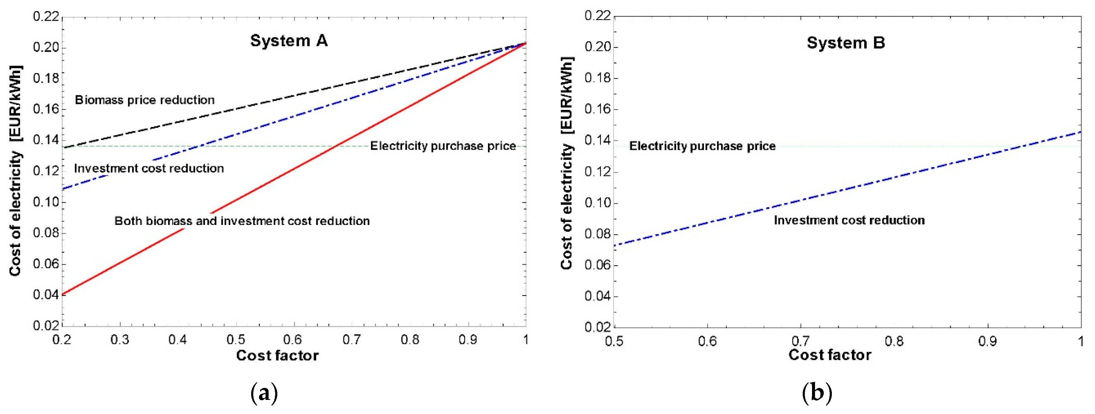
5.3. Sensitivity Analysis

Even though the economic analysis performed in Section 5.1 showed that systems A and B are presently not feasible from an economic viewpoint, the costs of the produced electricity are relatively low. Thus, in this section, we will analyze the factors influencing the costs of both systems.

As can be seen in Table 5, for system A, the investment cost of the solar field of parabolic trough collectors (153,690 EUR/year) represents almost 45% of the total annual investment cost (343,294 EUR/year) and 24% of the total annual cost (632,350 EUR/year). Regarding the operation costs, the energy cost of biomass is also quite high (217,738 EUR/year) and represents about 30% of the total annual cost. In the case of system B, the investment cost of the solar field of parabolic trough collectors (230,535 EUR/year) represents more than 45% of both the total annual investment costs and total annual costs. Note that, in system B, the total annual energy costs are very low, first, because there is no biomass consumption, and, second, because the electricity sale offsets about two thirds of the electricity purchase costs.

Since the investment costs (systems A and B) and the cost of biomass (system A only) accounted for significant shares of the total annual costs, we decided to assess the influence of the unit investment cost and the biomass purchase price on the cost of the electricity produced by the solar systems. The results presented in Figure 18 were obtained by modifying said costs independently and/or simultaneously. The line “Investment cost reduction” in system A was obtained by reducing the unit investment cost of the solar collectors (235 EUR/m²), the TES (65 EUR/kWh_t), the biomass boiler (315 EUR/kW_t) and the ORC (2000 EUR/kW_e) in proportion to the cost factor (a cost factor equal to one means that the cost remains unchanged, and a cost factor equal to 0.8 means that the cost of the considered component has experienced a 20% cost reduction, and so on), while keeping unchanged the cost of the rest of the plant components (chillers), energy resources and considered parameters (annual amortization factor and plant lifetime). Similarly, the line “Biomass price reduction” was obtained by reducing only the price of the biomass (0.0444 EUR/kWh). In contrast, the line “Both biomass and investment cost reduction” was obtained by simultaneously reducing the unit investment cost of the solar collectors, TES, biomass boiler, ORC and biomass price by applying the same cost factor. Clearly, only the effect of the unit investment cost of equipment (i.e., solar collectors, TES and ORC) was analyzed for system B, since there is no biomass boiler and no consumption of pellets.

For system A, the results show the significant influence of the biomass price. Only producing electricity with biomass is expensive due to the low energy efficiency of the ORC (about 20%), which means that the cost of each kWh of electricity is more than six times higher than the cost of each kWh of biomass consumed in the boiler. Note that the cost of the electricity produced is higher than the price of pellets divided by the efficiencies of the biomass boiler and the ORC. For this reason, reducing the biomass purchase cost has a significant effect on the cost of the electricity produced in system A. Nevertheless, a notable reduction in the biomass price (about 80%) is required to reach the electricity cost of the electricity produced in system A, which is similar to the price of electricity (0.1363 EUR/kWh) purchased from the grid. Reducing the investment cost of equipment (concentrating on the parabolic trough solar collectors, TES, biomass boiler and ORC) has a higher influence. Thus, in system A, it is possible to reach an electricity production cost lower than the electricity purchase price by reducing about 60% the investment cost. Combining both factors, with a reduction of 35% in the investment cost of equipment (concentrating parabolic trough solar collectors, TES, biomass boiler and ORC) and in the price of biomass, the cost of electricity produced would be lower than the price of electricity purchased.

For system B, in which the electricity cost is close to the electricity purchase price, with less than a 10% reduction in the investment cost of equipment (concentrating parabolic trough solar collectors, TES and ORC), it would already be possible to produce electricity at a lower cost than the electricity purchased from the grid.

Taking into account only the main parameters with the biggest influences, the obtained results show that, if properly optimized, a solar-based parabolic trough integrated with TES and ORC cogeneration plants, with possible hybridization using biomass, could become competitive in the medium term, provided that the significant cost reduction trend of this type of technology is maintained, which is expected for the next few years [20].

6. Conclusions

The technical feasibility of two novel solar-based PTC–ORC cogeneration systems, producing power and cooling only, and designed to cover the annual energy demands of a commercial center located in Zaragoza (Spain), has been proven. The commercial center considered herein, despite its high energy consumption, had a very low or null heat demand, which is a common situation in some kinds of buildings, such as commercial centers, depending, among other things, on their geographical location.

The analyzed cogeneration systems consist of solar parabolic trough collectors integrated with thermal energy storage, an Organic Rankine Cycle, and vapor compression mechanical chillers. System A is hybridized with a biomass boiler that supports solar thermal production and allows full load operation of the ORC throughout the solar system’s operating time. System B, on the other hand, is not hybridized with biomass. For this reason, the installed capacities of the solar system and ORC are larger, and it is considered that the ORC can modulate, operating at partial load, in order to produce the electrical requirements of the commercial center (electricity for cooling production and electricity demand). Both systems were connected to the electrical grid, regarded as an auxiliary system, thereby selling the surplus electricity, and purchasing the required electricity when needed.

The present work was developed by applying a systematic procedure to obtain the preliminary sizing of the plant components considering commercially available pieces of equipment. Moreover, a detailed physical simulation of the operation of the system throughout the day and the year was also performed, capturing its hourly, daily, and monthly dynamic behavior, considering: (i) the variations in ambient temperature, solar radiation, and thermal energy production, among others; and (ii) the modelling of the different pieces of equipment based on technical data and the investment costs of commercially available devices.

The technical feasibility analysis was complemented by simplified economic and environmental analyses. From an economic viewpoint, the proposed solar-based cogeneration systems were not competitive with conventional systems, in which all required electricity is purchased from the grid. The configuration without biomass hybridization (system B) was more economically interesting than the one with a biomass boiler (system A), producing electricity at 0.1458 EUR/kWh, which is only 7% more expensive than the electricity purchase price in Spain. This was mainly due to the elimination of the purchase of biomass pellets, at the expense of the operational reliability provided by a dispatchable renewable energy source (i.e., biomass) and of a simpler operating strategy due to the partial load operation of the ORC in system B. All things considered, the results are promising and reveal the systems’ potential interest and competitiveness in the short to medium term, particularly in a context in which external environmental costs could also be considered. From an environmental viewpoint, the proposed PTC–ORC systems present considerable benefits, contributing significantly to the decarbonization of energy production, and achieving a very high renewable fraction. Note that the plants’ main energy resources were renewable energies (i.e., solar and biomass), and their auxiliary resource was grid electricity. Nevertheless, it would be advisable to develop this analysis by including the environmental burden associated with the equipment construction.

Future research efforts are required in order to develop optimized cogeneration and trigenerations systems that are mainly driven by renewable energies in terms of: (i) sizing; (ii) more appropriate energy integration schemes, considering the possibility of covering all energy services of a building (heating, cooling and electricity), implementing absorption chillers as well as thermal energy storage of the heating and cooling produced; and (iii) reducing the investment costs of these systems.

References

1. IEA. Exploring the Impacts of the Covid-19 Pandemic on Global Energy Markets, Energy Resilience, and Climate Change. Available online: https://www.iea.org/topics/covid-19 (accessed on 20 May 2020).
2. IRENA. Global Renewables Outlook: Energy Transformation 2050; International Renewable Energy Agency: Abu Dhabi, UAE, 2020. [Google Scholar]
3. EU Comission and Parliament. Directive 2018/844 of the European Parliament and of the Council of 30 May 2018 Amending Directive 2010/31/EU on the Energy Performance of Buildings and Directive 2012/27/EU on Energy Efficiency; Official Journal of the European Union: Brussels, Belgium, 2018; Volume 156, pp. 75–91. [Google Scholar]
4. Kavvadias, K.; Jiménez-Navarro, J.P.; Thomassen, G. Decarbonising the EU Heating Sector—Integration of Power and Heating Sector; Publications Office of the European Union: Luxembourg, 2019. [Google Scholar]
5. Eurostat Renewable Energy for Heating and Cooling. Available online: https://ec.europa.eu/eurostat/en/web/products-eurostat-news/-/DDN-20200211-1 (accessed on 23 May 2020).
6. Odyssee-Mure. Energy Efficiency Trends and Policies—Spain Energy Profile, April 2020. Available online: https://www.odyssee-mure.eu/publications/efficiency-trends-policies-profiles/spain-spanish.html (accessed on 5 June 2020).
7. Forrester, S.P. Residential Cooling Load Impacts on Brazil’s Electricity Demand. Master’s Thesis, University of Michigan, Ann Arbor, MI, USA, 2019. [Google Scholar]
8. Serra, L.M.; Lozano, M.A.; Ramos, J.; Ensinas, A.V.; Nebra, S.A. Polygeneration and efficient use of natural resources. Energy 2009, 34, 575–586. [Google Scholar] [CrossRef]
9. Grilo, M.M.D.S.; Fortes, A.F.C.; de Souza, R.P.G.; Silva, J.A.M.; Carvalho, M. Carbon footprints for the supply of electricity to a heat pump: Solar energy vs. electric grid. J. Renew. Sustain. Energy 2018, 10, 023701. [Google Scholar] [CrossRef]
10. Solano-Olivares, K.; Romero, R.J.; Santoyo, E.; Herrera, I.; Galindo-Luna, Y.R.; Rodríguez-Martínez, A.; Santoyo-Castelazo, E.; Cerezo, J. Life cycle assessment of a solar absorption air-conditioning system. J. Clean. Prod. 2019, 240, 118206. [Google Scholar] [CrossRef]
11. Ullah, K.R.; Saidur, R.; Ping, H.W.; Akikur, R.K.; Shuvo, N.H. A review of solar thermal refrigeration and cooling methods. Renew. Sustain. Energy Rev. 2013, 24, 499–513. [Google Scholar] [CrossRef]
12. Noro, M.; Lazzarin, R.M. Solar cooling between thermal and photovoltaic: An energy and economic comparative study in the Mediterranean conditions. Energy 2014, 73, 453–464. [Google Scholar] [CrossRef]
13. Wang, R.Z.; Ge, T.S. Advances in Solar Heating and Cooling; Woodhead Publishing: Cambridge, UK, 2016; ISBN 9780081003015. [Google Scholar]
14. IEA. Tracking Clean Energy Progress. Available online: https://www.iea.org/topics/tracking-clean-energy-progress (accessed on 23 May 2020).
15. Lovegrove, K.; Stein, W. Concentrating Solar Power Technology; Woodhead Publishing: Cambridge, UK, 2012; ISBN 9781845697693. [Google Scholar]
16. Fernández-García, A.; Zarza, E.; Valenzuela, L.; Pérez, M. Parabolic-trough solar collectors and their applications. Renew. Sustain. Energy Rev. 2010, 14, 1695–1721. [Google Scholar] [CrossRef]
17. Kasaeian, A.; Bellos, E.; Shamaeizadeh, A.; Tzivanidis, C. Solar-driven polygeneration systems: Recent progress and outlook. Appl. Energy 2020, 264, 114764. [Google Scholar]
18. Zourellis, A.; Perers, B.; Donneborg, J.; Matoricz, J. Optimizing Efficiency of Biomass—Fired Organic Rankine Cycle with Concentrated Solar Power in Denmark. Energy Procedia 2018, 149, 420–426. [Google Scholar] [CrossRef]
19. MicroSolar, I. Innovative Micro Solar Heat and Power System for Domestic and Small Business Residential Buildings. Available online: http://innova-microsolar.eu/ (accessed on 23 May 2020).
20. IRENA. Renewable Power Generation Costs in 2018; International Renewable Energy Agency: Abu Dhabi, UAE, 2018; ISBN 978-92-9260-040-2. [Google Scholar]
21. Camilo, F.M.; Castro, R.; Almeida, M.E.; Pires, V.F. Economic assessment of residential PV systems with self-consumption and storage in Portugal. Sol. Energy 2017, 150, 353–362. [Google Scholar] [CrossRef]
22. Cerino Abdin, G.; Noussan, M. Electricity storage compared to net metering in residential PV applications. J. Clean. Prod. 2018, 176, 175–186. [Google Scholar] [CrossRef]
23. Thiem, S.; Danov, V.; Metzger, M.; Schäfer, J.; Hamacher, T. Project-level multi-modal energy system design—Novel approach for considering detailed component models and example case study for airports. Energy 2017, 133, 691–709. [Google Scholar] [CrossRef]
24. Li, G.; Zheng, X. Thermal energy storage system integration forms for a sustainable future. Renew. Sustain. Energy Rev. 2016, 62, 736–757. [Google Scholar] [CrossRef]
25. FEMP. Climatización Urbana en las Ciudades Españolas; Red Española de Ciudades por el Clima: Madrid, Spain, 2015. [Google Scholar]
26. ADHAC. Censo de Redes de Calor y Frío 2019; Asociación de Empresas de Redes de Calor y Frío: Madrid, Spain, 2019. [Google Scholar]
27. Quoilin, S.; Van Den Broek, M.; Declaye, S.; Dewallef, P.; Lemort, V. Techno-economic survey of organic rankine cycle (ORC) systems. Renew. Sustain. Energy Rev. 2013, 22, 168–186. [Google Scholar] [CrossRef] [Green Version]
28. Macchi, E.; Astolfi, M. Organic Rankine Cycle (ORC) Power Systems; Woodhead Publishing: Cambridge, UK, 2016; ISBN 9780081005101. [Google Scholar]
29. Borunda, M.; Jaramillo, O.A.; Dorantes, R.; Reyes, A. Organic Rankine Cycle coupling with a Parabolic Trough Solar Power Plant for cogeneration and industrial processes. Renew. Energy 2016, 86, 651–663. [Google Scholar] [CrossRef]
30. Patel, B.; Desai, N.B.; Kachhwaha, S.S.; Jain, V.; Hadia, N. Thermo-economic analysis of a novel organic Rankine cycle integrated cascaded vapor compression–absorption system. J. Clean. Prod. 2017, 154, 26–40. [Google Scholar] [CrossRef]
31. Buonomano, A.; Calise, F.; Palombo, A.; Vicidomini, M. Energy and economic analysis of geothermal-solar trigeneration systems: A case study for a hotel building in Ischia. Appl. Energy 2015, 138, 224–241. [Google Scholar] [CrossRef]
32. Petrollese, M.; Cocco, D. Robust optimization for the preliminary design of solar organic Rankine cycle (ORC) systems. Energy Convers. Manag. 2019, 184, 338–349. [Google Scholar] [CrossRef]
33. Mascuch, J.; Novotny, V.; Vodicka, V.; Spale, J.; Zeleny, Z. Experimental development of a kilowatt-scale biomass fired micro—CHP unit based on ORC with rotary vane expander. Renew. Energy 2020, 147, 2882–2895. [Google Scholar] [CrossRef]
34. Prando, D.; Renzi, M.; Gasparella, A.; Baratieri, M. Monitoring of the energy performance of a district heating CHP plant based on biomass boiler and ORC generator. Appl. Therm. Eng. 2015, 79, 98–107. [Google Scholar] [CrossRef]
35. Algieri, A.; Morrone, P. Energetic analysis of biomass-fired ORC systems for micro-scale combined heat and power (CHP) generation. A possible application to the Italian residential sector. Appl. Therm. Eng. 2014, 71, 751–759. [Google Scholar] [CrossRef]
36. Chowdhury, M.T.; Mokheimer, E.M.A. Recent Developments in Solar and Low-Temperature Heat Sources Assisted Power and Cooling Systems: A Design Perspective. J. Energy Resour. Technol. 2019, 142, 040801. [Google Scholar] [CrossRef]
37. Wu, Q.; Ren, H.; Gao, W.; Weng, P.; Ren, J. Design and operation optimization of organic Rankine cycle coupled trigeneration systems. Energy 2018, 142, 666–677. [Google Scholar] [CrossRef]
38. Zhao, L.; Zhang, Y.; Deng, S.; Ni, J.; Xu, W.; Ma, M.; Lin, S.; Yu, Z. Solar driven ORC-based CCHP: Comparative performance analysis between sequential and parallel system configurations. Appl. Therm. Eng. 2018, 131, 696–706. [Google Scholar] [CrossRef]
39. Arteconi, A.; Del Zotto, L.; Tascioni, R.; Cioccolanti, L. Modelling system integration of a micro solar Organic Rankine Cycle plant into a residential building. Appl. Energy 2019, 251, 113408. [Google Scholar] [CrossRef]
40. Bellos, E.; Vellios, L.; Theodosiou, I.C.; Tzivanidis, C. Investigation of a solar-biomass polygeneration system. Energy Convers. Manag. 2018, 173, 283–295. [Google Scholar] [CrossRef]
41. Karellas, S.; Braimakis, K. Energy-exergy analysis and economic investigation of a cogeneration and trigeneration ORC-VCC hybrid system utilizing biomass fuel and solar power. Energy Convers. Manag. 2016, 107, 103–113. [Google Scholar] [CrossRef]
42. Boyaghchi, F.A.; Heidarnejad, P. Thermoeconomic assessment and multi objective optimization of a solar micro CCHP based on Organic Rankine Cycle for domestic application. Energy Convers. Manag. 2015, 97, 224–234. [Google Scholar] [CrossRef]
43. Garcia-Saez, I.; Méndez, J.; Ortiz, C.; Loncar, D.; Becerra, J.A.; Chacartegui, R. Energy and economic assessment of solar Organic Rankine Cycle for combined heat and power generation in residential applications. Renew. Energy 2019, 140, 461–476. [Google Scholar] [CrossRef]
44. Roumpedakis, T.C.; Loumpardis, G.; Monokrousou, E.; Braimakis, K.; Charalampidis, A.; Karellas, S. Exergetic and economic analysis of a solar driven small scale ORC. Renew. Energy 2020, 157, 1008–1024. [Google Scholar] [CrossRef]
45. Pantaleo, A.M.; Camporeale, S.M.; Miliozzi, A.; Russo, V.; Shah, N.; Markides, C.N. Novel hybrid CSP-biomass CHP for flexible generation: Thermo-economic analysis and profitability assessment. Appl. Energy 2017, 204, 994–1006. [Google Scholar] [CrossRef]
46. Perers, B.; Sørensen, P.-A.; Kvist, P.; Neergaard, T.B.; Jensen, J.R.; Sørensen, P.A.; From, N.; Sallaberry, F. A CSP Plant Combined with Biomass CHP Using Orc-Technology in Brønderslev Denmark. In Proceedings of the EuroSun 2016, Palma de Mallorca, Spain, 11–14 October 2016; International Solar Energy Society: Freiburg, Germany, 2016; pp. 1–7. [Google Scholar]
47. Tian, Z.; Perers, B.; Furbo, S.; Fan, J. Thermo-economic optimization of a hybrid solar district heating plant with flat plate collectors and parabolic trough collectors in series. Energy Convers. Manag. 2018, 165, 92–101. [Google Scholar] [CrossRef] [Green Version]
48. De la Energía, E.P. Biomasa y Solar, la Micro-Trigeneración Perfecta para Generar Electricidad y Energía Térmica de Calor y frío. Available online: https://elperiodicodelaenergia.com/biomasa-y-solar-la-micro-trigeneracion-perfecta-para-generar-electricidad-y-energia-termica-de-calor-y-frio/ (accessed on 23 May 2020).
49. SAM. System Advisor Model (SAM); National Renewable Energy Laboratory (NREL): Golden, CO, USA, 2018.
50. Turboden Organic Rankine Cycle Technology. Available online: www.turboden.eu (accessed on 21 February 2020).
51. Daikin Optimización del Sistema en Aplicaciones de Enfriadoras Condensadas por Aire. Available online: www.daikin.eu (accessed on 26 May 2020).
52. Wagner, M.; Gilman, P. Technical Manual for the SAM Physical Trough Model; National Renewable Energy Laboratory (NREL): Golden, CO, USA, 2011.
53. Hernández, A. Design and Analysis of Electricity and Air Conditioning Polygeneration System for a Shopping Center Located in Zaragoza; Graduate Project; School of Engineering and Architecture, Universidad de Zaragoza: Zaragoza, Spain, 2019. [Google Scholar]
54. Pina, E.; Lozano, M.A.; Serra, L.M.; Ballerini, C.; Verda, V.; Lazaro, A. Large scale solar cooling/parabolic trough-ORC-biomass polygeneration system for a shopping centre. In Proceedings of the IEA SHC Task 55 “Towards the Integration of Large SHC Systems into DHC Networks”, 6th Expert Meeting, Almería, Spain, 8–10 April 2019. [Google Scholar]
55. TRNSYS. A Transient System Simulation Tool. Available online: http://sel.me.wisc.edu/trnsys/ (accessed on 21 February 2019).
56. Wagner, M.J.; Blair, N.; Dobos, A. A Detailed Physical Trough Model for NREL’s Solar Advisor Model. In Proceedings of the SolarPACES 2010, Perpignan, France, 21–24 September 2010; pp. 1–11. [Google Scholar]
57. Obernberger, I.; Hammerschmid, A.; Forstinger, M. Techno-economic evaluation of selected decentralised CHP applications based on biomass combustion with steam turbine and ORC processes. In Proceedings of the IEA Bioenergy Task 32 Project; BIOS BIOENERGIESYSTEME GmbH: Graz, Austria, 2015; pp. 1–75. [Google Scholar]
58. Swegon; Cobalt, W. Chiller y Bombas de calor Agua/Agua 172–1527 kW. Available online: http://www.swegon.com (accessed on 21 February 2020).
59. Forristall, R. Heat Transfer Analysis and Modeling of a Parabolic Trough Solar Receiver Implemented in Engineering Equation Solver; National Renewable Energy Laboratory (NREL): Golden, CO, USA, 2003.
60. Therminol Heat Transfer Fluids by Eastman. Available online: https://www.therminol.com/ (accessed on 15 May 2020).
61. Meteotest. Meteonorm Software. Available online: http://www.meteonorm.com/ (accessed on 26 May 2020).
62. EES. Engineering Equation Solver Software; F-Chart Software: Madison, WI, USA, 2020. [Google Scholar]
63. Ballerini, C. Thermal Analysis of a Solar Parabolic Trough—ORC—Biomass Cogeneration Plant of Electricity and Cooling Applied to a Shopping Centre. Master’s Thesis, Politecnico di Torino, Turin, Italy, 2018. [Google Scholar]
64. Kurup, P.; Turchi, C.S. Parabolic Trough Collector Cost Update for the System Advisor Model (SAM); Technical Report NREL/TP-6A20-65228; National Renewable Energy Laboratory (NREL): Golden, CO, USA, 2015; pp. 1–40. [CrossRef] [Green Version]
65. Bruno, J.C.; López-Villada, J.; Letelier, E.; Romera, S.; Coronas, A. Modelling and optimisation of solar organic rankine cycle engines for reverse osmosis desalination. Appl. Therm. Eng. 2008, 28, 2212–2226. [Google Scholar] [CrossRef]
66. Desai, N.B.; Bandyopadhyay, S. Thermo-economic analysis and selection of working fluid for solar organic Rankine cycle. Appl. Therm. Eng. 2016, 95, 471–481. [Google Scholar] [CrossRef]
67. RSMeans. Mechanical Cost Data 2018. Available online: https://www.rsmeans.com/ (accessed on 26 May 2020).
68. EUROSTAT. Eurostat Database. Available online: http://ec.europa.eu/eurostat/data/database (accessed on 15 January 2019).
69. IDAE. Informe de Precios de la Biomasa para Usos Térmicos. 2019. Available online: https://www.idae.es/sites/default/files/estudios_informes_y_estadisticas/informe_precios_biomasa_usos_termicos_3t_2019.pdf (accessed on 26 May 2020).
70. IDAE. Factores de Emisión de CO2 y Coeficientes de paso a Energía Primaria de Diferentes Fuentes de Energía Final Consumidas en el Sector de Edificios en España. 2014, pp. 1–31. Available online: https://energia.gob.es/desarrollo/EficienciaEnergetica/RITE/Reconocidos/Reconocidos/Otros%20documentos/Factores_emision_CO2.pdf (accessed on 26 May 2020). (In Spanish).
Figure 1. Monthly thermal cooling energy demand percentage of the commercial center (%) [51].
Energies 13 04807 g001
Figure 2. Hourly occupancy indices on working days (top) and holidays (bottom) [51].
Energies 13 04807 g002
Figure 3. Hourly thermal cooling demands (kWht) of the commercial center throughout the year: (a) working days; (b) holidays.
Energies 13 04807 g003
Figure 4. Hourly load profiles of electric demand (excluding cooling production) of the commercial center on working days and holidays.
Energies 13 04807 g004
Figure 5. Simplified diagram of the analyzed parabolic trough–ORC–biomass cogeneration system. Adapted from Wagner and Gilman [52].
Energies 13 04807 g005
Figure 6. Simplified scheme of the solar collector assemblies (SCA). Adapted from Wagner and Gilman [52].
Energies 13 04807 g006
Figure 7. Receiver model: (a) thermal energy balance; (b) thermal resistance model [59].
Energies 13 04807 g007
Figure 8. Organic Rankine Cycle (ORC) energy efficiency at partial load operation [50].
Energies 13 04807 g008
Figure 9. Annual energy balance of the hybrid solar parabolic trough–ORC–biomass plant (system A), MWh/year.
Energies 13 04807 g009
Figure 10. System A. Solar field hourly profiles obtained with System Advisor Model (SAM) [49] of indicated physical magnitudes for four selected months.
Energies 13 04807 g010
Figure 11. System A. Monthly thermal energy (left side) and hourly thermal energy (right side) of the solar system and boiler.
Energies 13 04807 g011
Figure 12. System A. Electricity produced, bought and sold on working days. Monthly values (left side) and hourly values (right side).
Energies 13 04807 g012
Figure 13. System A. Electricity produced, bought and sold on holidays. Monthly values (left side) and hourly values (right side).
Energies 13 04807 g013
Figure 14. Annual energy balance of the solar parabolic trough–ORC analyzed plant (system B), MWh/year.
Energies 13 04807 g014
Figure 15. System B. Monthly thermal energy (left side) and hourly thermal energy (right side) of the solar field.
Energies 13 04807 g015
Figure 16. System B. Electricity produced, bought and sold in working days. Monthly values (left side) and hourly values (right side).
Energies 13 04807 g016
Figure 17. System B. Electricity produced, bought and sold in holidays. Monthly values (left side) and hourly values (right side).
Energies 13 04807 g017
Figure 18. Sensitivity analysis of the cost of electricity produced as a function of the biomass price and investment cost (parabolic trough collector (PTC), thermal energy storage (TES), biomass boiler and ORC) in (a) system A; (b) system B (biomass boiler and biomass price are not considered for system B).
Energies 13 04807 g018