Faulty Feeder Detection Method Based on VMD–FFT and Pearson Correlation Coefficient of Non-Power Frequency Component in Resonant Grounded Systems

Abstract

Through analyzing the transient components and transient characteristics in transient zero-sequence current (TZSC), a novel fault feeder detection method based on the transient correlation of non-power frequency components (NPFCs) for the resonant grounded system is proposed. Firstly, using variational mode decomposition combined with fast Fourier transformation (VMD–FFT) to decompose the TZSC, by removing the power frequency components and noise signals, the transient NPFCs can be obtained. Secondly, to reflect the overall changing trend between faulty and healthy currents, the moving average filter is introduced to smooth the NPFCs; in this way, the fault transient features can be accurately revealed. Finally, the faulty feeder can be detected by comparing the threshold with the maximum difference value of comprehensive correlation coefficient of NPFCs. The detection results show that the proposed fault detection method can accurately select the faulty feeder; it is unaffected by fault resistances, fault phase angles, etc. Moreover, the detection method can resist noise interference.

1. Introduction

Among the existing operation modes of power distribution networks, the resonance grounding system is most widely used. Single-phase ground (SPG) faults occur most frequently in this type of network, accounting for more than 70% of all fault types. When SPG faults occur in resonant grounding systems, existing line selection techniques have relatively low accuracy due to factors such as unstable arcs and weak fault characteristics [1,2,3,4].

Many researchers have explored the selection of SPG faulty lines. Existing line selection methods are active [5,6,7] or passive [8,9,10,11,12,13,14,15,16,17,18,19,20,21,22]. Active line selection does not depend on the fault current, but requires additional primary equipment and is greatly affected by the ground resistance, giving these methods limited applicability. Passive line selection methods can be divided into steady state and transient state categories. Steady state methods [8,9,10] mainly include amplitude comparison, phase comparison, zero sequence power, and zero sequence admittance techniques. These approaches are susceptible to factors such as operation modes.

The current signal at the moment of fault encompasses rich transient characteristic information. The transient method [11,12,13,14,15] is favored by many scholars. Liu et al. [16] used the Prony algorithm to extract the transient main frequency components of individual lines. This method requires no settings but has low anti-noise capacity. Shu et al. [17] used the peak–valley features of zero-sequence current morphology for faulty line selection; this approach does not work well under small-angle fault conditions. Xue et al. [18] proposed a line selection method based on the difference in projection coefficients of the zero-sequence current on the zero-sequence voltage. The selection ability for low-resistance faults showed room for improvement. Wang et al. [19] used wavelet transformation to decompose a transient zero-sequence current (TZSC), but the choice of wavelet basis function showed undue influence on the decomposition results. Wang et al. [20] introduced a novel cut-in point for fault detection issues; the power component can be calculated based on the fast Fourier transformation (FFT) method. Firstly, the power frequency component is eliminated by FFT, and then the non-power frequency component (NPFC) is obtained; the final results show that the fault detection method has high accuracy. However, when the TZSC contains harmonics, the detection method needs to be further verified.

The Empirical Mode Decomposition (EMD) algorithm has been proposed for faulty line selection to resolve the above problems [21,22,23]. EMD does not require a priori selection of the basis function and can directly decompose the input signal. Shu et al. [22] first used EMD to decompose a TZSC and obtain the high-frequency components. The faulty line was determined based on the magnitude of the correlation coefficient of the waveform. Though effective to some extent, this EMD decomposition process is prone to modal aliasing.

A faulty line selection method based on variational mode decomposition combined with fast Fourier transformation (VMD–FFT) and the Pearson correlation coefficient was developed in this study to improve the accuracy of faulty line selection in resonant grounded systems. The VMD first adaptively calculates the center frequency of the signal to decompose the zero-sequence current of each outgoing line into intrinsic mode functions (IMFs), intuitively reflecting their compositions. The low-frequency IMFs of each outgoing line are then subjected to FFT analysis to obtain the power frequency component of the fault signal. Then, the NPFCs of each outgoing line are obtained, smoothed, and subjected to a Pearson correlation analysis. Finally, the faulty line is determined. This prevents the inaccurate separation of power frequency components otherwise caused by modal aliasing and boundary effects in traditional algorithms.

2. Composition and Characteristics of TZSC for Faults

When a SPG fault occurs in the resonant ground system, the equivalent circuit for the transient analysis is as shown in Figure 1. In this circuit, $U_{0f}$ represents the zero-sequence voltage source, $R_0$ and $L_0$ are the equivalent grounding resistance and inductance of the zero-sequence circuit, $R_P$ and $L_P$ are the equivalent resistance and equivalent inductance of the arc suppression coil, and $C$ is the total ground capacitance of the system.

As shown in Figure 1, the circuit equation is:

$$R_0{i}_C{+L}_0\frac{d{i}_c}{dt}+\frac{1}{C}{\displaystyle {\int }_0^t{i}_C}dt=U_m\sin ({\omega }_{b}t+\phi )$$

(1)

$$R_P{i}_L+L_P\frac{d{i}_L}{dt}=U_m\sin ({\omega }_{b}t+\phi )$$

(2)

where $i_C$ and $i_L$ are the transient capacitance current and inductance current; $U_m$ is the relative ground voltage amplitude of the system; ${\omega }_b$ is the reference frequency; and $\phi$ is the initial phase angle of the power supply voltage at the moment of grounding.

According to Equations (1) and (2), $i_0$, the TZSC flowing through the fault point can be determined as:

$$i_0=i_L+i_C=I_L\cos \phi e^{-\frac{t}{{\tau }_L}}+(I_C-I_L)\cos ({\omega }_{b}t+\phi )+I_C(\frac{{\omega }_f}{{\omega }_b}\sin \phi \sin {\omega }_{b}t-\cos \phi \cos {\omega }_{f}t)e^{-\delta t}$$

(3)

where $I_L$ and $I_C$ are the amplitudes of the inductor current and capacitor current, ${\omega }_f$ and $\delta$ are the transient free oscillation frequency and attenuation coefficient, $\delta =1/{\tau }_c$, ${\tau }_c$ is the attenuation time constant of the capacitor current, and ${\tau }_L$ is the attenuation time constant of the inductor current.

Equation (3) indicates that for a resonant grounding system, the fault TZSC is mainly composed of attenuated DC components, power frequency AC components, and transient high-frequency components. The attenuated DC component is generated by the loop between the fault point and the arc suppression coil. Its magnitude varies with the initial phase angle $\phi$ and reaches its maximum when $\phi$ = 0.

Due to the compensation effect of the arc suppression coil, the zero-sequence currents of the faulty line and the non-faulty line have a capacitive constraint relationship in the power frequency component. No line can be selected without the fault characteristics. In the transient high-frequency component, under the effect of the same zero-sequence voltage, the direction of the high-frequency component of the non-faulty line moves from the bus to the line. The amplitude is mainly determined by the equivalent capacitance to the ground of each line. By contrast, the high-frequency component of the faulty line is equal to the sum of all non-faulty lines moving from the line to the bus and with an amplitude greater than that of the non-faulty line.

When using the TZSC, the power frequency component seriously affects the accuracy of faulty line selection as a disturbance variable. The disturbance in the power frequency component in the zero-sequence current should be eliminated. In the early stage of the fault, non-faulty lines have similar NPFC waveforms in the TZSC. Additionally, faulty and non-faulty lines have significant differences in amplitude and polarity. Faulty lines can be identified based on the correlation of the NPFCs of the TZSC.

3. Line Selection Theory and Process

3.1. Principles of Variational Mode Decomposition

VMD is a widely used, non-linear, pre-scaled signal processing algorithm that was first proposed in 2014. In essence, the VMD algorithm transforms the signal decomposition problem into a constrained optimization problem. The optimal solution obtained is the decomposed single-component amplitude-modulated–frequency-modulated (AM–FM) signal. In other words, VMD decomposes the TZSC signal $i_{0j}$ of line j into K intrinsic modal functions $u_k(t)$ with a center angle frequency ${\omega }_k$, where K is the preset number of modal components. Unlike EMD decomposition, VMD defines each IMF as an AM–FM function $u_k(t)$:

$$u_k(t)=A_k(t)\cos ({\mathsf{\varphi }}_k(t))$$

(4)

where instantaneous amplitude value $A_k(t)\ge 0$; ${\omega }_k(t)={\mathsf{\varphi }}_k^{\prime }(t)$.

The step-wise operation of the VMD algorithm is as follows [24].

(1)

The TZSC signal $i_{0j}$ is subjected to Hilbert transformation, resulting in the analytical signals of the K modal component $u_k(t)$ and the $u_k(t)$ single-sided spectrum:

$$\left[\delta (t)+\frac{j}{\pi t}\right]u_k(t)$$

(5)

where $\delta (t)$ is the impulse function.

(2)

The frequency spectrum of each mode is modulated to the base frequency band:

$$\left\{\left[\delta (t)+\frac{j}{\pi t}\right]u_k(t)\right\}{e}^{-j{\omega }_{k}t}$$

(6)

(3)

The square $L^2$ norm of the gradient of Formula (6) is calculated. The bandwidth of each modal signal was estimated. The variational problem is established as follows:

$$\{\begin{array}{c}\underset{\left\{u_k\right\},\left\{{\omega }_k\right\}}{\min }\left\{{\displaystyle \sum _{k=1}^K{\Vert {\partial }_t\left\{\left[\delta (t)+\frac{j}{\pi t}\right]u_k(t)\right\}{e}^{-j{\omega }_{k}t}\Vert }_2^2}\right\}\\ s.t.{\displaystyle \sum _{k=1}^K{u}_k}=f\end{array}$$

(7)

where ${\partial }_t$ is the partial derivative of $t$; $\left\{u_k\right\}:=\left\{u_1,u_2,\dots ,u_K\right\}$; $\left\{{\omega }_k\right\}:=\left\{{\omega }_1,{\omega }_2,\dots ,{\omega }_K\right\}$.

(4)

In order to solve the above constrained variational problem, the quadratic penalty factor $\mathsf{\alpha }$ and the Lagrangian multiplication operator $\lambda (t)$ can be introduced into Equation (7) to turn it into a non-constrained variational problem. The extended Lagrangian expression is:

$$L(\left\{u_k\right\},\left\{{\omega }_k\right\},\lambda ):=\mathsf{\alpha }{\displaystyle \sum _{k=1}^K{\Vert {\partial }_t\left\{\left[\mathsf{\delta }(t)+\frac{j}{\pi t}\right]u_k(t)\right\}{e}^{-j{\omega }_{k}t}\Vert }_2^2}+{\Vert f(t)-{\displaystyle \sum _{k=1}^K{u}_k(t)}\Vert }_2^2+\langle \lambda (t),f(t)-{\displaystyle \sum _{k=1}^K{u}_k(t)}\rangle$$

(8)

(5)

The alternate direction method of multipliers (ADMM) is applied to solve the extended Lagrangian expression. The specific steps are:

(a)

Initialize variables $\left\{{\widehat{u}}_k^1\right\},\left\{{\omega }_k^1\right\},{\widehat{\lambda }}^1,n$;

(b)

Execute cycles: $n=n+1$;

(c)

Update $u_k$, ${\omega }_k$ and $\lambda$;

$${\widehat{u}}_k^{n+1}\left(\omega \right)\leftarrow \frac{\widehat{f}\left(\omega \right)-{\displaystyle \sum _{i\ne k}^K{\widehat{u}}_i^{}\left(\omega \right)}+\frac{\widehat{\lambda }(\omega )}{2}}{1+2\alpha {(\omega -{\omega }_k^{})}^2}$$

(9)

$${\omega }_k^{n+1}\leftarrow \frac{{\displaystyle {\int }_0^{\infty }\omega }{\left|{\widehat{u}}_k^{}\left(\omega \right)\right|}^{2}d\omega }{{\displaystyle {\int }_0^{\infty }{\left|{\widehat{u}}_k^{}\left(\omega \right)\right|}^{2}d\omega }}$$

(10)

$${\widehat{\lambda }}^{n+1}\left(\omega \right)\leftarrow {\widehat{\lambda }}^n\left(\omega \right)+\mathsf{\tau }\left(\widehat{f}\left(\omega \right)-{\displaystyle \sum _{k=1}^K{\widehat{u}}_k^{n+1}\left(\omega \right)}\right)$$

(11)

where $\mathsf{\tau }$ is the noise margin parameter.

(d)

Steps b–d are repeated until the iteration termination conditions are met:

$${\displaystyle \sum _{k=1}^K({\Vert {\widehat{u}}_k^{n+1}-{\widehat{u}}_k^n\Vert }_2^2/{\Vert {\widehat{u}}_k^n\Vert }_2^2)}<e$$

(12)

where $e$ is the condition for iteration termination.

In order to discuss the decomposition effect of VMD on TZSC, a previously described ideal TZSC signal [25] is taken as an example for verification:

$$\begin{array}{l}x(t)=x_1(t)+x_2(t)+x_3(t)+x_4(t)+\epsilon (t)\\ x_1(t)=5.6\cos (2\pi \times 50t+{60}^{°})\\ x_2(t)=40e^{-56t}\cos (2\pi \times 250t+{30}^{°})\\ x_3(t)=72e^{-102t}\cos (2\pi \times 315t)\\ x_4(t)=10e^{-5.5t}\end{array}$$

(13)

where $x_1(t)$ is the power frequency signal; $x_2(t)$ is the fifth harmonic signal; $x_3(t)$ is the non-integer harmonic signal; $x_4(t)$ is the attenuated DC component; and $\epsilon (t)$ is the white noise signal.

The ideal signal can be generated from the characteristics of the TZSC when a SPG fault occurs in a resonant grounding system. VMD was used here to analyze $x(t)$ while the number of decomposition levels K = 3 and the secondary penalty factor $\alpha$ = 2000. The resulting decomposed IMF1, IMF2, and IMF3 are shown in Figure 2.

As shown in Figure 2, IMF1 is a low-frequency component containing power frequency components and attenuated DC components. IMF2 is a transient high-frequency attenuation component and IMF3 is noise signal. VMD effectively separated low-frequency components, high-frequency components, and white noise components in an ideal TZSC in this case.

3.2. Separation of Power Frequency Components by FFT

As shown in Figure 2, VMD cannot directly separate the power frequency components of the zero-sequence current. Further processing is needed. Steady-state harmonic signal analysis is usually conducted via FFT. In order to accurately obtain NPFCs and avoid any interference from transient signals, the second power frequency period of IMF1 was subjected here to FFT analysis. First, an FFT analysis of the second power frequency cycle of IMF1 was performed to obtain power frequency components; IMF1 (minus the obtained power frequency component) and IMF2 were then added to obtain the NPFC of the TZSC.

The actual NPFC are shown in the blue solid line in Figure 3 with the ideal zero sequence current signal as an example. An FFT analysis was performed on the IMF1 shown in Figure 2 to obtain the NPFC of the ideal zero-sequence current, as marked with a red dashed line in Figure 3.

In Figure 3, the actual NPFC coincide with the NPFC obtained by the proposed algorithm. This method can accurately separate the power frequency components and noise signals, ultimately revealing the NPFC of the transient zero sequence current.

3.3. Data Smoothing and Pearson Correlation Coefficient

To highlight the overall trend characteristics of NPFCs of faulty lines and non-faulty lines, the paper selects a moving average filter to smooth the NPFCs, and the results obtained can better describe the trend characteristics of NPFCs.

The NPFCs of TZSCs $i_{0i}$ and $i_{0j}$ were selected for faulty and non-faulty lines, as shown in Figure 4a,c, to smooth the element point at a certain moment as an example. This point was placed as the center and g elements (odd number) were selected as an interval. (g = 199 was found by trial and error to meet the line selection requirements of this study.) The elements in the interval were fitted by the second-order polynomial to obtain a weighted regression curve; this step was repeated for the remaining element points to obtain their respective weighted regression curves. Finally, the centers of all regression curves were connected together to obtain a smoothed signal curve.

The results before and after smoothing the NPFCs are shown in Figure 4. This method appears to perform well without altering the overall trend of $i_{0i}$ and $i_{0j}$, which is conducive to subsequent correlation analysis.

The Pearson correlation coefficient is based on a concept proposed by Karl Pearson. It is typically used to measure the degree of correlation between two variables resulting in a value between −1 and 1 [26,27]. It is calculated as follows:

$${\rho }_{ij}=\frac{{\displaystyle \sum _{a=1}^N(i_{0i}(a)-\overline{i_{0i}})(i_{0j}(a)-\overline{i_{0j}})}}{\sqrt{{\displaystyle \sum _{a=1}^N{(i_{0i}(a)-\overline{i_{0i}})}^2}}\sqrt{{\displaystyle \sum _{a=1}^N{(i_{0j}(a)-\overline{i_{0j}})}^2}}}$$

(14)

where N is the number of sampling points; $\overline{i_{0i}}$ and $\overline{i_{oj}}$ are the average values of N elements of $i_{0i}$ and $i_{0j}$, respectively.

Pearson correlation has good analytical performance for the linear correlation. However, when signals are interfered by the noises, the strong correlation between actual signals may be broken. As a result, the Pearson correlation coefficients may be close to 0 [28]. The smoothing method can filter the high-frequency noises and restore the original characteristics of the actual signals. Therefore, the smoothing method can help to accurately reflect the true Pearson correlations between faulty NPFC and non-faulty NPFCs. The Pearson correlation coefficient of the two lines $i_{0i}$ and $i_{0j}$ is −0.2901 before processing (Figure 4) and that of ${\rho }_{ij}$ after smoothing is −0.9980. This suggests that smoothing highlights the overall trend characteristics of NPFCs in faulty and non-faulty lines, which yields an accurate correlation line selection.

3.4. Line Selection Method and Process

(1)

The zero-sequence voltage of the system busbar, $U_0$, is first continuously monitored on-line. When $U_0$ exceeds 0.15 $U_N$, the line selection device is activated and the transient zero sequence current of the m circuit is recorded. The TZSC of two power frequency cycles after the fault of the m circuit line is then VMD decomposed to obtain the corresponding IMF component. The NPFCs of each outgoing line are obtained (Section 3.2) and the NPFCs of each line are smoothed and filtered to obtain $H_i(i=1,2,\dots m)$.

(2)

The Pearson correlation coefficient of the first 1/4 power frequency cycle H_i following the fault is calculated to obtain the correlation coefficient matrix M:

$$\mathit{M}=\left[\begin{array}{cccc}{\rho }_{11}& {\rho }_{12}& \dots & {\rho }_{1m}\\ {\rho }_{21}& {\rho }_{22}& \dots & {\rho }_{2m}\\ ⋮& ⋮& \ddots & ⋮\\ {\rho }_{m1}& {\rho }_{m2}& \dots & {\rho }_{mm}\end{array}\right]$$

(15)

(3)

This matrix M is normalized to obtain the comprehensive correlation coefficient P of each line. The comprehensive correlation coefficient $P_i$ of the i-th circuit relative to other m−1 circuits is calculated as follows:

$$P_i=\frac{1}{m-1}{\displaystyle \sum _{j=1,j\ne i}^m{\rho }_{ij}}$$

(16)

(4)

The absolute value S of the difference between the maximum value $P_{max}$ and the minimum value $P_{min}$ of the comprehensive correlation coefficient is calculated. If S is greater than the set threshold $P_{set}$ (0.3 in this case), the corresponding line of $P_{min}$ is judged as faulty; otherwise, it is judged as a bus fault.

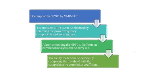
A flow chart of this faulty line selection process is given in Figure 5.

4. Simulation Analysis

4.1. Simulation Modeling

A cable hybrid system simulation model was established in the electromagnetic transient simulation software ATP (3.8, SINTEF Energy Research, Norway), as shown in Figure 6, which includes four lines:

• the line L₁ is a 13 km overhead line;
• the line L₂ is a hybrid of a 4 km cable line and a 12 km overhead line;
• the line L₃ is a hybrid of a 3 km cable line and a 10 km overhead line;
• the line L₄ is a 6 km cable line.

The line impedance parameters [29] are shown in

Table 1. Impedance parameters of transmission line.

Line Types	Sequence	Resistance (Ω/km)	Inductance (mH/km)	Capacitance (nF/km)
Overhead line	positive-sequence	0.17	1.2	9.697
	zero-sequence	0.23	5.48	6
Cable line	positive-sequence	0.193	0.442	143
	zero-sequence	1.93	5.48	143

.

The transformers in this setup are 110/10.5 kV. The resistance of the single-phase neutral point coil on the high-voltage side is 0.40 Ω. The inductance is 12.2 Ω. The resistance of the single-phase coil on the low-voltage side is 0.006 Ω and the inductance is 0.183 Ω. The excitation current is 0.672 Ω, the excitation flux is 202.2 Wb, and the magnetic circuit resistance is 400 kΩ. The delta connection method was used in all cases, ZL = 400 + j20 Ω. Overcompensation was simulated in the arc suppression coil grounding system with a 10% overcompensation degree and 1.2819 H arc suppression coil inductance. The resistance value of the arc suppression coil is 10% of the reactance value, 40.2517 Ω. The model sampling frequency fs = 10⁵ Hz. The period T = 0.02 s. The SPG fault occurred at 0.02 s in the simulation, which was 0.06 s long in total.

4.2. Simulation Case Analysis

4.2.1. Overhead Line Fault

The A-phase grounding fault on the line L₁ at a distance of 5 km from the bus line is discussed here as an example. The initial phase angle of the fault is 90° and the grounding resistance is 100 Ω. After Gaussian white noise with a signal to noise ratio (SNR) of 10 dB was injected into the collected signal, the zero-sequence current waveform of the line was derived as shown in Figure 7.

As shown in Figure 7, the zero-sequence current of each line contains obvious power frequency components and transient high-frequency components. The maximum amplitude of the faulty line reaches about 150 A, which is much larger than that of the non-faulty line. The lines have opposing polarities. The TZSC of each outgoing line was decomposed in three layers using VMD, resulting in each outgoing line IMF1, as shown in Figure 8.

As shown in Figure 8, the IMF1 of line L₁ has the largest amplitude and the IMF1 of each outgoing line is composed mainly of low-frequency components, with power frequency components as the main components. FFT analysis can be used to separate the power frequency components.

As shown in Figure 9, IMF2 is dominated by transient high-frequency components without power frequency components. This indicates that VMD can decompose low-frequency components and high-frequency components with favorable decomposition effects.

As shown in Figure 10, IMF3 is the noise signal of each line. In effect, VMD can accurately decompose the interference noise of each line and has a good denoising ability. After VMD decomposition was completed, H_j was obtained by the line selection method discussed above, as shown in Figure 11.

Figure 11 is the NPFC H_j obtained here after smoothing and filtering the NPFC of each line. The Pearson correlation coefficient of each outgoing line H_j was calculated to form the correlation coefficient matrix M:

$$\mathit{M}=\left[\begin{array}{rrrr}\hfill 1& \hfill -0.9985& \hfill -0.9984& \hfill -0.9976\\ \hfill -0.9985& \hfill 1& \hfill 1.0000& \hfill 0.9965\\ \hfill -0.9984& \hfill 1.0000& \hfill 1& \hfill 0.9964\\ \hfill -0.9976& \hfill 0.9965& \hfill 0.9964& \hfill 1\end{array}\right]$$

The comprehensive correlation coefficient P = [−0.9982, 0.3327, 0.3327, 0.3318] was calculated after normalization. S is much larger than $P_{set}$ in this case. As a result, the line corresponding to the minimum value, line L₁ can be judged as a faulty line. The line selection result is accurate.

4.2.2. Cable Line Fault

The A-phase grounding fault with a grounding resistance of 500 Ω at the cable line L₄, 3 km away from the bus, is presented here as an example, where the initial phase angle of the fault is 90°. Gaussian white noise with an SNR of 30 dB was injected into the collected zero sequence current of each outgoing line as shown in Figure 12.

The NPFC H_j after the smoothing and filtering of each outgoing line is shown in Figure 13.

The comprehensive correlation coefficient P = [0.4486, 0.4512, 0.4516, −0.6473] was obtained after the Pearson correlation coefficient was calculated. S was greater than $P_{set}$ in this case, so the line corresponding to the minimum value (L₄) can be judged as faulty. The line selection result is accurate.

4.2.3. Bus Fault

A SPG fault with a grounding resistance of 100 Ω was next imposed at the bus bar, where the initial phase angle of the fault is 0°. Gaussian white noise with an SNR of 30 dB was injected into the collected zero-sequence current of each outgoing line as shown in Figure 14.

As shown in Figure 14, when the ground fault occurred on the bus, the initial polarities of the zero-sequence current of each line were the same. The NPFC H_j of each smoothed and filtered outgoing line is shown in Figure 15.

As shown in Figure 15, the polarities of all outgoing lines H_j are the same. The comprehensive correlation coefficient P = [0.9937 0.9974 0.9975 0.9974] can be calculated accordingly. S is less than $P_{set}$ here, so a bus fault is identified. The line selection result is accurate.

5. Applicability Analysis

The fault resistance, initial phase angle of the fault, intensity of the injected noise, and fault location were changed in succession for the purposes of further analysis. The proposed algorithm was used to obtain the the absolute value S of the difference between the comprehensive correlation coefficient P of the NPFCs of each line and the maximum and minimum values. The results, as presented below, confirm the applicability of the faulty line selection method based on VMD–FFT NPFC correlation analysis.

The SPG fault of the overhead line L₁ is presented here as an example. At this time, the initial phase angle of the fault is 90°, the fault is 5 km away from the bus, the SNR is 30 dB, and the fault resistance increases from 1 Ω to 1000 Ω. The changes in the NPFCs P and S of each feeder are shown in Figure 16.

As the resistance increases, the comprehensive correlation coefficients of lines L_2, L₃, and L₄ become basically approximated. Although the comprehensive correlation coefficient of line L₁ increases to some extent, it is still smaller than the other three-circuit lines. The S value indicates that line L₁ is the faulty line. These results show that the proposed algorithm can be used to accurately select the faulty line as the grounding resistance changes.

5.2. Changing Initial Fault Phase Angle

When a SPG fault occurs on the overhead line L₁, the fault resistance is 5 Ω, and the fault is 5 km away from the bus. As the initial phase angle of the fault changes from 0° to 90°, the changes in P and S of the NPFCs of each outgoing line are as shown in Figure 17.

As shown in Figure 17, when the initial phase angle of the fault changes, the faulty line can be accurately selected based on the P and S of each feeder.

5.3. Changing Fault Location

The SPG fault of the cable line L₄ was next given a grounding resistance of 100 Ω, initial phase angle of the fault of 0°, and faults 2 km, 3 km, 4 km, and 5 km from the bus, respectively. The changes in P and S of the NPFCs of all outgoing lines are shown in Figure 18.

As shown in Figure 18, when the fault location changes, the faulty line can still be quickly and accurately selected based on the P and S values of each feeder.

5.4. Changing Injected Noise Intensity

When a SPG fault occurs on the cable hybrid line L₃, the fault resistance is 100 Ω, the initial phase angle of the fault is 90°, the fault is 3 km, and the SNRs are −10 dB, 0 dB, 10 dB, 20 dB, and 30 dB, respectively, the changes in P and S of the NPFCs of each feeder are as shown in Figure 19.

As shown in Figure 19, when the intensity of the noise changes, the P and S of each feeder change very slightly. This suggests that the proposed method can be used to accurately select faulty lines with high noise tolerance.

6. Comparison Analysis

In order to verify the superiority and effectiveness of the proposed method, another two commonly used fault detection methods are compared, the one is based on the EMD algorithm and correlation analysis [22], the second one is based on the Prony algorithm and correlation analysis [16].

When the SPG fault occurs on the hybrid line L₂, and the fault initial phase angle is 90°, the fault resistance is 1 Ω, 500 Ω, and 1000 Ω, respectively. The final fault detection results and the comparisons are listed in

Table 2. Comparisons with the existing fault detection methods.

Detection Method	Fault Resistances	Line Selection Criterion	Fault Detection Result
Proposed method	1	[0.3316, −0.9959, 0.3320, 0.3273]	L2
	500	[0.3529, −0.9254, 0.3537, 0.3523]	L2
	1000	[0.3916, −0.7947, 0.3813, 0.3897]	L2
EMD-based method	1	[0.0320, −0.6848, 0.0245, 0.0137]	L2
	500	[−0.0845, −0.3926, −0.2264, −0.3814]	L2
	1000	[−0.1229, −0.3933, −0.3592, −0.3065]	Bus
Prony-based method	1	[−0.0106, −0.3176, −0.0058, −0.2611]	L2
	500	[0.0723, −0.1725, 0.0809, −0.3103]	L4
	1000	[−0.0165, −0.3049, −0.0085, −0.3171]	L4

.

As shown in Table 2, when the fault resistance is equal to 1 Ω, the three methods can detect the fault line accurately. When the fault resistance is equal to 500 Ω, both the proposed method and EMD-based method achieve accurate fault detection results, while the Prony-based method misjudges the faulty line. When the resistance increases to 1000 Ω, only the proposed method can accurately detect the faulty line, while the other two give the wrong results. Therefore, when a SPG fault occurs with a large grounding resistance, and the fault detection results based on the EMD algorithm and the Prony algorithm are no longer reliable, the superiority and effectiveness of the proposed method can be verified.

VMD and FFT were combined in this study to accurately separate power frequency components and noise signals in a TZSC. The proposed algorithm was found to be more accurate than EMD-based method and Prony-based method.

7. Conclusions

By analyzing the composition and characteristics of the TZSC of a resonant grounding system, a novel faulty line selection method was established in this study based on the correlation analysis of NPFCs via VMD–FFT. The main conclusions of this work can be summarized as follows.

• VMD and FFT are combined to prevent any inaccurate separation of power frequency components caused by modal aliasing and boundary effects, and to provide a sound basis for subsequent line selection.
• The moving average filter smoothes and filters the NPFCs to reveal the overall trend of the NPFCs. This highlights the correlations between faulty lines and non-faulty lines.
• The proposed line selection algorithm is relatively unaffected by factors such as fault resistance and fault initial phase angle and shows strong anti-noise characteristics.

References

- Barik, M.A.; Gargoom, A.; Mahmud, M.A. A decentralized fault detection technique for detecting single phase to ground faults in power distribution systems with resonant grounding. IEEE Trans. Power Deliv. 2018, 33, 2462–2473. [Google Scholar]
- Wang, X.; Gao, J.; Wei, X.; Zeng, Z.; Wei, Y.; Kheshti, M. Single line to ground fault detection in a non-effectively grounded distribution network. IEEE Trans. Power Deliv. 2018, 33, 3173–3186. [Google Scholar]
- Shao, W.; Bai, J.; Cheng, Y.; Zhang, Z.; Li, N. Research on a Faulty Line Selection Method Based on the Zero-Sequence Disturbance Power of Resonant Grounded Distribution Networks. Energies 2019, 12, 846. [Google Scholar] [CrossRef]
- Guo, Z.; Yao, J.; Yang, S.; Zhang, H.; Mao, T.; Dong, T. A new method for non-unit protection of power transmission lines based on fault resistance and fault angle reduction. Int. J. Electr. Power Energy Syst. 2014, 55, 760–769. [Google Scholar] [CrossRef]
- Zhu, K.; Ni, J.; Zhang, R. A New Approach for Fault Location in Resonant Grounded System Based on Active Disturbance Technology. Power Syst. Technol. 2016, 40, 1881–1887. [Google Scholar]
- Zhu, K.; Wang, Y.; Ni, J. Application of active disturbance technology in faulty line selection of arc suppression coil grounding system. Electr. Power Autom. Equip. 2017, 37, 189–196. [Google Scholar]
- Qi, Z.; Zhuang, S.; Liu, Z. Analysis on Distribution Network Fault Location Method Based on Parallel Resistance Disturbed Signal Injection. Autom. Electr. Power Syst. 2018, 42, 195–200. [Google Scholar]
- Zhang, Z.X.; Liu, X.; Piao, Z.L. Fault line detection in neutral point ineffectively grounding power system based on phase-locked loop. IET Gener. Transm. Distrib. 2014, 8, 273–280. [Google Scholar]
- Lin, X.N.; Huang, J.G.; Ke, S.H. Faulty feeder detection and fault self-extinguishing by adaptive Petersen coil control. IEEE Trans. Power Deliv. 2011, 26, 1290–1291. [Google Scholar] [CrossRef]
- Lin, X.; Sun, J.; Kuran, I.; Zhao, F.; Li, Z.; Li, X.; Yang, D. Zero-sequence compensated admittance based faulty feeder selection algorithm used for distribution network with neutral grounding through Peterson-coil. Int. J. Electr. Power Energy Syst. 2014, 63, 747–752. [Google Scholar] [CrossRef]
- Liu, M.; Wang, Y.; Zeng, X. Novel method of fault line selection based on characteristic analysis of transient phase-current. Proc. CSU EPSA 2017, 29, 30–36. [Google Scholar]
- Shu, H.; Gong, Z.; Tian, X.; Dong, J.; Li, S. Single Line-to-ground Fault Line Selection Based on Fault Characteristic Frequency Band and Morphological Spectrum. Power Syst. Technol. 2019, 43, 1041–1053. [Google Scholar]
- Guo, M.F.; Yang, N.C. Features-clustering-based earth fault detection using singular-value decomposition and fuzzy c-means in resonant grounding distribution systems. Int. J. Electr. Power Energy Syst. 2017, 93, 97–108. [Google Scholar] [CrossRef]
- Peng, N.; Kai, Y.; Rui, L. Single-Phase-to-Earth Faulty Feeder Detection in Power Distribution Network Based on Amplitude Ratio of Zero-Mode Transients. IEEE Access 2019, 7, 117678–117691. [Google Scholar] [CrossRef]
- Guo, M.; Zeng, X.; Chen, D.; Yang, N. Deep-Learning-Based Earth Fault Detection Using Continuous Wavelet Transform and Convolutional Neural Network in Resonant Grounding Distribution Systems. IEEE Sens. J. 2018, 18, 1291–1300. [Google Scholar] [CrossRef]
- Liu, M.; Fang, T.; Jiang, Y. A new correlation analysis approach to fault line selection based on transient main-frequency components. Power Syst. Prot. Control 2016, 44, 74–79. [Google Scholar]
- Shu, H.; Huang, H.; Tian, X. Fault Line Selection in Resonant Earthed System Based on Morphological Peak-Valley Detection. Autom. Electr. Power Syst. 2019, 43, 228–233. [Google Scholar]
- Xue, Y.; Li, J.; Chen, X. Faulty feeder selection and transition resistance identification of high impedance fault in a resonant grounding system using transient signals. Proc. CSEE 2017, 37, 5037–5048. [Google Scholar]
- Wang, X.; Gao, J.; Wei, X. A novel fault line selection method based on improved oscillator system of power distribution network. Math. Probl. Eng. 2014, 2014, 1–19. [Google Scholar] [CrossRef]
- Wang, X.; Wei, X.; Yang, D.; Song, G.; Gao, J.; Weri, Y.; Zeng, Z.; Wang, P. Fault feeder detection method utilized steady state and transient components based on FFT backstepping in distribution networks. Int. J. Electr. Power Energy Syst. 2020, 114, 105391. [Google Scholar]
- Zha, C.; Wang, C.; Wei, Y. A new method of the resonant grounding system fault line detection based on EMD. Power Syst. Prot. Control 2014, 42, 100–104. [Google Scholar]
- Liu, M.; Fang, T.; Jiang, Y. Fault Line Selection Method Based on Correlation Analysis of High-frequency Components. Proc. CSU EPSA 2017, 29, 101–106. [Google Scholar]
- Hou, S.; Guo, W. Optimal Denoising and Feature Extraction Methods Using Modified CEEMD Combined with Duffing System and Their Applications in Fault Line Selection of Non-Solid-Earthed Network. Symmetry 2020, 12, 536. [Google Scholar] [CrossRef]
- Dragomiretskiy, K.; Zosso, D. Variational Mode Decomposition. IEEE Trans. Signal Process. 2014, 62, 531–544. [Google Scholar] [CrossRef]
- Kang, X.; Liu, X.; Suonan, J. New method for fault line selection in non-solidly grounded system based on matrix pencil method. Autom. Electr. Power Syst. 2012, 36, 88–93. [Google Scholar]
- Shangguan, X.; Qin, W.; Xia, F. Pole-to-ground Fault Protection Scheme for MMC Multi-terminal Flexible DC Distribution Network Based on Pearson Correlation of Transient Voltage. High Volt. Eng. 2020, 46, 1740–1749. [Google Scholar]
- Zang, J.; Xiong, G.; Meng, K. An improved probabilistic load flow simulation method considering correlated stochastic variables. Int. J. Electr. Power Energy Syst. 2019, 111, 260–268. [Google Scholar] [CrossRef]
- Jiang, F.; Feng, Z.; Zhu, J. Applied research to assess envaporator performances in ORC system by Pearson correlation coefficient. Acta Energ. Sol. Sin. 2019, 40, 2732–2738. [Google Scholar]
- Yang, D.; Wei, X.; Wen, B. Fault line selection method based on sparse decomposition and comprehensive measure values for distribution network. High Volt. Eng. 2017, 43, 1526–1534. [Google Scholar]
Figure 1.
Transient equivalent circuit for the single-phase ground (SPG) fault.
Figure 2.
VMD decomposition results with use of ideal transient zero-sequence current (TZSC). (a) Ideal TZSC; (b) intrinsic mode function (IMF)1; (c) IMF2; (d) IMF3.
Figure 3.
Comparisons for two calculated non-power frequency components (NPFCs).
Figure 4.
Smoothing results based on the moving average filter. (a) NPFC of before smoothing; (b) NPFC of after smoothing; (c) NPFC of before smoothing; (d) NPFC of after smoothing.
Figure 5.
Fault detection flow chart.
Figure 6.
ATP simulation model for radial distribution network.
Figure 7.
TZSCs for SPG fault. (a) Lian L1; (b) Lian L2; (c) Lian L3; (d) Lian L4.
Figure 8.
IMF1 components of each outgoing line. (a) Lian L1; (b) Lian L2; (c) Lian L3; (d) Lian L4.
Figure 9.
IMF2 components of each outgoing line. (a) Lian L1; (b) Lian L2; (c) Lian L3; (d) Lian L4.
Figure 10.
IMF3 components of each outgoing line. (a) Lian L1; (b) Lian L2; (c) Lian L3; (d) Lian L4.
Figure 11.
NPFCs after smoothing. (a) Lian L1; (b) Lian L2; (c) Lian L3; (d) Lian L4.
Figure 12.
TZSCs for SPG fault (Case 2). (a) Lian L1; (b) Lian L2; (c) Lian L3; (d) Lian L4.
Figure 13.
NPFCs after smoothing (Case 2). (a) Lian L1; (b) Lian L2; (c) Lian L3; (d) Lian L4.
Figure 14.
TZSCs for SPG fault (Case 3). (a) Lian L1; (b) Lian L2; (c) Lian L3; (d) Lian L4.
Figure 15.
NPFCs after smoothing (Case 3). (a) Lian L1; (b) Lian L2; (c) Lian L3; (d) Lian L4.
Figure 16.
S and P of each feeder for different fault resistances. (a) P of each feeder for different fault resistances; (b) S of different fault resistances.
Figure 17.
S and P of each feeder for different fault phase angles. (a) P of each feeder for different fault phase angles; (b) S of different fault phase angles.
Figure 18.
S and P of each feeder with distance variation. (a) P of each outgoing line with distance variation; (b) S of distance variation.
Figure 19.
S and P of each feeder for different signal to noise ratios (SNRs). (a) P of each feeder for different SNRs; (b) S of different SNRs.