Comparison of Electricity Spot Price Modelling and Risk Management Applications

Abstract

In dealing with sharp changes in electricity prices, contract planning is considered as a vital risk management tool for stakeholders in deregulated power markets. In this paper, dynamics of spot prices in Turkish electricity market are analyzed, and predictive performance of several models are compared, i.e., time series models and regime-switching models. Different models for derivative pricing are proposed, and alternative portfolio optimization problems using mean-variance optimization and conditional value at risk (CVaR) are solved. Expected payoff and risk structure for different hedging strategies for a hypothetical electricity company with a given demand are analyzed. Experimental studies show that regime-switching models are able to capture electricity characteristics better than their standard counterparts. In addition, evaluations with various risk management models demonstrate that those models are highly competent in providing an effective risk control practice for electricity markets.

1. Introduction

In many countries around the world, electricity markets were been liberalized in the late 20th century. Subsequently, integrated state-owned electricity companies have been separated into specialized individual market participants. Before the liberalization, the power sector in most of these countries was not free to competition, and cost-based pricing was applied where prices were calculated by regulators using generation, transmission, and distribution costs of electricity. As a result, there were no price risks in the electricity market. However, as a result of liberalization, electricity price risk has appeared as one of the most critical financial risks for the market participants. In particular, both the electricity generation and distribution companies face these new uncertainty factors and therefore higher financial risk.

Electricity markets have attracted the attention of both researchers and practitioners due to the major changes in the market environment. Studies on electricity markets aim to understand the unique attributes of electricity and help the market participants interpret the characteristics of this product. Studies on electricity markets can be divided into two significant streams concerning our work. The first stream is modeling the electricity price process, and the second is the risk management of electricity portfolios. In this paper, we aim to deal with those two issues.

Electricity, as a trading commodity of the power markets, has a distinguishing characteristic that it is fundamentally non-storable and behaves different form other commodities according to [1]. Besides, demand for electricity is highly volatile due to the seasonality of customer usage as stated by [2]. The change in demand depends on both deterministic and stochastic factors. An example of the deterministic effect is the time of the day or day of the week. However, the stochasticity of the market depends on different factors, such as business cycles or weather. Electricity spot prices display cyclic patterns on different frequencies, such as daily, weekly, and annual cycles. As suggested by [3], disruptive effects like unexpected outages at power plants or uncertainty at transmission lines add complexity and reduce predictability. Extreme price changes due to disruptive events can be modeled using jump processes. These spikes are usually short-lived and unexpected, and after jump periods, a mean-reverting characteristic is usually observed.

There are several various approaches to electricity price modeling. Main types of models can be classified as fundamental, game-theoretic, stochastic, and time-series models [4]. Different methods are generally used for different applications; therefore, it is not easy to compare them. In fundamental models, the supply-demand relationship is used to simulate future prices. A general model for all the participants in the market is generated to find the marginal production costs and demand prices, and the equilibrium price is calculated for different scenarios of production and order levels. Full supply and demand curves are modeled by [5] to derive prediction intervals for short and medium term forecasting. Furthermore, [6,7] extend their approach for long term forecasting. These models are used for long term price estimation by using all the information on potential power plants and usage scenarios. In game-theory models, the market players are modeled as independent agents who optimize their bid prices. These models are used to analyze the strategic decisions of market participants. Initially, [8] built an agent based model to test different market designs. The authors of [9] investigate the optimal strategies of suppliers in an electricity market using Nash equilibrium. Both of the fundamental and game-theoretic models are equilibrium type models rather than pricing models. Since they have diverse objectives, hence these varied methods are not easy to compare. This paper aims to compare the effectiveness of stochastic and time-series models from a risk analysis perspective.

The stochastic models—which is also called reduced form models by [10]—consist of jump diffusions or Markov regime switching models. Derivatives for electricity contracts are priced by [11] using Merton jump-diffusion model. On the other hand, [12] used hidden Markov models for regime switching properties to model the movements in prices of US electricity markets. In a more recent study, Ref. [13] uses a modelling approach where they integrate the deterministic seasonal components with regime-switching feature based stochastic factors through higher order hidden Markov models. Statistical time series methods are used to model the future price through a mathematical function of the previous prices. In addition to the pure price information of exogenous factors, such as supply-demand figures, or weather variables can be used. Most basic statistical model applied to electricity prices is the exponential smoothing method in [14]. A widely used time series method is the linear approach such as different types of autoregressive moving average (ARMA-type) models. Recent studies using time series modelling in energy markets include [15,16,17,18]. In [10] another type of model is defined as the computational intelligence models. Recent advances in machine learning has also affected the electricity pricing literature with vast amount of new studies [19]. The main methods used can be counted as neural networks [20,21], support vector machines [22], deep learning [23,24,25] and ensemble methods [26,27].

The households and usually the small and medium enterprises buy their electricity with fixed prices, so the electricity providers absorb the entire risk of volatile spot prices. Therefore, they have to use derivative contracts for risk management purposes to fix their electricity purchasing costs. Financial products such as futures, forwards, or options are some instances of instruments that allow people to make decisions by their risk preferences. Ref. [28] provides a broad review of electricity derivatives that are commonly in use. In this study, we assume the companies use forward contracts. Forward contracts are agreements between buyers and sellers, making those players exchange an asset or commodity, in this context, electricity, with pre-specified price in a predefined future time.

Since the retailers are private companies the main objective of a retailer is to minimize the expected cost for a given level of the risk parameter selected.There are various approaches to define the risk. The conditional value at risk (CVaR) model, used by [29] in the context of single stage portfolio optimisation, is preferred due to its linear structure in the scenario based modelling. In the context of electricity spot price uncertainty, Ref. [30] first used CVaR criterion in addition to several risk criteria such as worst return and mean semi-deviation below the mean return and solved a multiple criteria optimization problem for a single stage. In [31], authors have defined a two-stage stochastic integer programming model in order to devise an optimal power contract portfolio from the perspective of a generation company. In contrast to multi-stage models they define the second stage for balancing the demand. In a multi-stage environment, Ref. [32] deals with the portfolio selection problem for an electricity retailer using derivative contracts and applied robust optimization using decision rules to the problem. They do not incorporate any other risk parameter in their model. In [33], authors propose a model with minimizing the cost and the CVaR in a multi-stage stochastic programming framework and compare the performance of the predefined model with the hedge-and-forget case. A scenario tree of stochastic spot prices is generated using a simple autoregressive model, and a tree-based solution procedure is applied. Their experiments show that the multi-stage stochastic programming method outperforms the hedge and forget approach. However, in their multi-stage framework the contracts are only valid in a single stage; therefore, each stage can be solved independently. In our model we use future contracts with longer maturity period. In recent studies CVaR is used for different problems in the risk management in energy markets context. For example, Ref. [34] model the risks for a virtual power plant, Ref. [35] examine the supplier selection problem for large customers, or [36] risk averse natural gas generator operation in a micro-grid.

The main contributions of this study are listed below.

• Different models for electricity pricing have been proposed, and their regime-switching counterparts have been driven. All models are compared for both the in-sample and out-sample performance.
• CVaR based multi-stage risk management model for a distributor company is developed, and differences between single and multi-stage models are examined.
• The performance of different pricing and simulation models for risk hedging purposes have been investigated
• Risk-return trade-off for different levels of risk averseness is analyzed.

The rest of this study is formed as follows. Electricity price models are introduced in Section 2. Portfolio optimisation models are developed in Section 3. Empirical results for the estimation of the model parameters and the optimisation results are provided in Section 5. This paper is finalized with the conclusion section.

2. Electricity Price Models

The price processes are modelled via stochastic and econometric time-series approaches as they are often used to capture short term price movements. Besides, those models allow to add external factors such as the business cycles, weather conditions and fuel prices. Main stochastic (or financial) models are geometric Brownian motion models with possible addition of regime switching components, jump processes and mean reverting processes. Similarly, time series models can be categorized as autoregressive and mean reverting models with heteroscedastic components. In both time series and financial models there exists deterministic components such as trend variables and seasonal cycles. The deterministic components are modelled in the same way for all the models analysed. For that reason the deterministic component is removed from historical prices to obtain stochastic parts. Following that, the parameters for the proposed models are estimated.

In the literature, various approaches can be found for extracting deterministic components of price series for financial variables. Following [2], spot price of electricity $X\left(t\right)$ can be represented as a sum of two independent components, i.e., deterministic component $X^d\left(t\right)$ and stochastic component $X^s\left(t\right)$ ($X\left(t\right)=X^d\left(t\right)+X^s\left(t\right)$). Deterministic component is equivalent to sum of two parts defined as trend $X^t\left(t\right)$ and seasonal $X^c\left(t\right)$. Trend components represent the increase (or decrease) in prices throughout the years due to the changes in supply of the electricity or consumption conditions. In this paper, a non-linear trend as the average price in a yearly moving window is used. In particular trend at time t is defined as

$$X^t\left(t\right)=\frac{1}{8760}\sum _{s=t-4380}^{t+4380}X\left(s\right).$$

(1)

Obtained historical data and the literature on prices suggest three main cycles in electricity prices. Those cycles are (i) daily cycle that is effected by change in the levels of demand during daytime and night time; (ii) weekly cycle represents differences between weekdays and weekends and (iii) yearly cycle reflects seasonal usage differences. Yearly cycle is defined as a sum of trigonometric functions given in Equation (2). Annual cycle explains seasonal variation in prices and changes with the higher and lower price periods of the year.

$$X^y\left(t\right)=\sum _{i=1}^k{\beta }_k^y\left(cos(2\pi i(t-{\phi }_k^y)/365/24)\right)$$

(2)

where k is the number of components, ${\beta }_k^y$ is the magnitude of the component and ${\phi }_k^y$ is the phase difference between the data and the component. According to [37] the set ${\{exp\left(2\pi \kappa i\right)\}}_{\kappa \in Z}$ is an orthonormal basis and any periodic function can be approximated by a sum of trigonometric functions arbitrarily good. Here as the computational part is applied to the Turkish market, hourly price data is used. If the price is determined half hourly in the market then the denominator inside the cosine function in Equation (2) should be changed by 48 instead of 24. Using a cosine function provides a better estimation for yearly data since number of variables to be estimated is smaller.

The weekly cycle is modelled through a step function that changes with respect to day of the week as in Equation (3).

$$X^w\left(t\right)=\sum _{i=1}^6{\alpha }_i{W}_i\left(t\right)$$

(3)

In Equation (3), $W_i\left(t\right)$ is an indicator function. To clarify, $W_i\left(t\right)$ is equal to zero if time t is at day i where Monday is defined as day one. Here, Sunday is the base day for which all the indicator functions are equal to zero. Daily cycle is also defined by using orthonormal basis as in (2). Daily cycle function for hourly based prices is given in Equation (4).

$$X^g\left(t\right)=\sum _{i=1}^k{\beta }_k^g\left(cos(2\pi i(t-{\phi }_k^g)/24)\right)$$

(4)

Seasonal and trend components of the prices are combined and overall deterministic part is given in Equation (5).

$$X^d\left(t\right)=X^t\left(t\right)+X^y\left(t\right)+X^w\left(t\right)+X^g\left(t\right).$$

(5)

In this paper the same form for deterministic component $X^d\left(t\right)$ is used for all the alternative approaches of price models.

2.1. Mean Reverting Model

In times of supply disruptions it is common to observe sudden price spikes in electricity markets, and after these spikes the price usually reverts to mean levels. According to [38] most of the energy spot prices have mean reverting characteristic. Specifically for electricity, speed of mean reversion in prices series distinguishes electricity from others. Among all financial time series electricity spot prices are perhaps the one with the fastest rates of mean reversion [39]. Mean reversion process (or Ornstein-Uhlenbeck process as defined in [40]) can be formulated using stochastic differential equation (SDE) and is stated in Equation (6).

$$d{X}^s\left(t\right)=\kappa (\mu -X^s\left(t\right))dt+\sigma d{W}_t$$

(6)

In Equation (6), $\mu$ is the long term average mean for the stochastic component, $\kappa$ is the mean reversion rate and $W_t$ is the standard Brownian motion. After applying Ito’s Lemma to Equation (6) one can obtain the discrete time version of mean reversion process. As suggested by [41] discrete time mean reversion equation is derived as in Equation (7).

$$X^s\left(t\right)=X^s(t-1)e^{-\kappa \delta }+\mu \left(1-e^{-\kappa \delta }\right)\sigma \sqrt{\frac{1-e^{-2\kappa \delta }}{2\kappa }}{\epsilon }_t$$

(7)

In Equation (7), $\delta$ is set to one hour and ${\epsilon }_t$ is a standard normal random variable. Mean reverting model has similar characteristics with an autoregressive (AR) process with lag equal to 1.

An important assumption for mean reversion process is about normality of residuals. However, as noted by [42] normality assumption does not hold in electricity prices. Electricity price processes are heavy-tailed and positively skewed. Reason of that outcome is the instantaneous jumps in the prices. Jumps in electricity prices are usually modelled by using a Poisson error component in addition to mean reverting model in (6). Let $dq$ be Poisson factor responsible for jumps arrivals and let J be the jump heights, then mean reversion process with jump can be written as Equation (8).

$$d{X}^s\left(t\right)=\kappa (\mu -X^s\left(t\right))dt+\sigma d{W}_t+ln\left(J\right)dq.$$

(8)

The variable J is assumed to be log-normally distributed where $ln\left(J\right)>0$ that can be interpreted as positive jumps. In the discrete version of mean reversion process, jump process is added as a random variable that takes zero value with probability p and value of a log-normal random variable with probability $1-p$ (Equation (9)).

$$X^s\left(t\right)=X^s(t-1)e^{-\kappa \delta }+\mu \left(1-e^{-\kappa \delta }\right)\sigma \sqrt{\frac{1-e^{-2\kappa \delta }}{2\kappa }}{\epsilon }_t+ln\left(J\right)dq.$$

(9)

Required probability values are estimated by counting the number of jumps in the process. Besides, distribution of J is estimated from the size of jumps.

2.2. ARMA Model

In addition to mean reversion processes, autoregressive moving average (ARMA) processes are also widely used to model the electricity prices [42]. ARMA process consists of two parts where the autoregressive components consider the last p previous prices, and the mean average part is based on the last q error terms. Although there exists different extensions for ARMA processes, the standard ARMA process used in this paper can be defined as given in Equation (10).

$$X^s\left(t\right)=\sum _{i=1}^p{\alpha }_i{X}^s(t-i)+\sum _{j=1}^q{\beta }_j{ϵ}_{t-j}+{ϵ}_t$$

(10)

In Equation (10), ${ϵ}_t$ is a normal random variable. ARMA process assumes that the residuals are normal with independent and identically distributed. It is a well-known fact that the electricity residuals do not satisfy this assumption [43]. That issue is a consequence of the jump processes and the heteroscedastic variance. Usually after the jump occurrences, volatility stays high since the markets are often nervous about the equilibrium price levels. Using Generalized AutoRegressive Conditional Heteroskedasticity (GARCH) models those types of market behaviour can be effectively modelled.

Several forms of GARCH modeling are proposed in the literature. In this paper the definition suggested by [44] is used. Formula for GARCH (p, q) model (p is the order of the volatility terms and q is the order of the residual terms) is given by Equation (11).

$${\sigma }_t^2=\omega +\sum _{z=1}^p{\alpha }_z^g{\sigma }_{t-z}^2+\sum _{z=1}^q{\beta }_z^g{\epsilon }_{t-z}^2.$$

(11)

It is usually common to set p and q values equal to one. In Equation (11), $\omega$ is a constant, ${\alpha }_z^g$ and ${\beta }_z^g$ are the autoregressive and moving average coefficients, ${\sigma }_{t-z}$ stands for time-variant variance and ${\epsilon }_{t-z}$ represents residual terms.

2.3. Regime Switching Models

Although the jump process explains the sudden movements in the price shifts of stock market variables, they are not adequate to model the price dynamics of electricity. In electricity price series a positive jump caused by interruptions is followed by some period of high prices and afterwards a negative jump as a result of the system repair [45]. Stochastic jump is considered as poor at explaining the sudden change of regime in prices. Use of mean reversion with jump process has its drawbacks since the reverting rate after the jumps and in normal periods needs to be different. It is not possible to distinguish normal operating times from the post-catastrophic events. This induces high estimation errors.

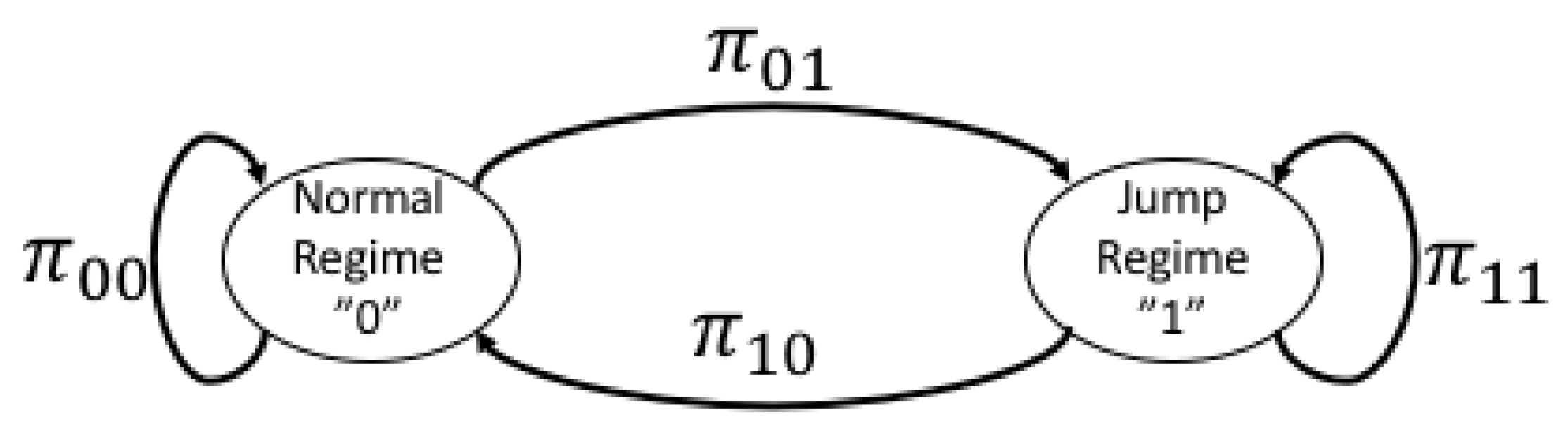
Regime switching models aid to avoid this problem by introducing different regimes for different market conditions. The idea of the regime-switching models is that the time series behaves differently in different economic environments by defining an environmental variable, i, the state or regime. Although it is possible to estimate models with n different regimes, in the literature usually two or three states are suggested for regime switching time series models. One of the regimes model ordinary conditions whereas the other(s) models disruption periods which may include the price spikes or the negative prices. Here, two different regimes, i.e., base regime (State 0) and peak regime (State 1) are used. A sample diagram used in regime switching models is illustrated in Figure 1.

The regime switching electricity market can be modelled using discrete time Markov chains since prices set with hourly time intervals. In order to model a market using Markov chains one needs to estimate the transition probability matrix. Probability of the market’s regime being the same between consecutive periods is denoted by ${\pi }_{ii}$ for $i=0,1$. More specifically, ${\pi }_{00}$ (${\pi }_{11}$) is the probability that a base regime (peak regime) continues given the previous one is base (peak regime). Transition matrix is defined in Equation (12).

$$P=\left[\begin{array}{cc}{\pi }_{00}& 1-{\pi }_{00}\\ 1-{\pi }_{11}& {\pi }_{11}\end{array}\right]$$

(12)

Note that, ${\pi }_{01}=1-{\pi }_{00}$ is probability of transition of the market from base to peak regimes and ${\pi }_{10}=1-{\pi }_{11}$ is from peak to base state.

The parameters for the Markov process are calculated using historical stochastic residues of electricity prices. The process at time t is assumed to be in peak regime if $X^s\left(t\right)$ is $3\sigma$ higher than the mean level. After classifying the past data into different regimes transition probabilities ${\pi }_{ij}$ are calculated as the probability of switching to or remaining in the respective regime between two time steps through historical data.

Regime switching approach are applied to mean reversion, ARMA and GARCH models. It is assumed that the process in base regime is mean reverting, ARMA, or GARCH and estimate the parameters using the historical data for the base regime. Then the parameters of peak regime using the corresponding historical price residuals are calculated.

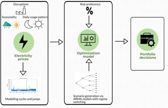
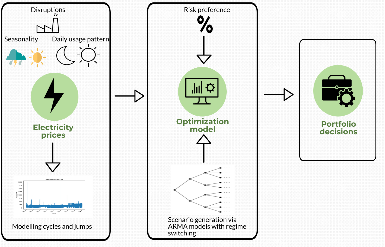
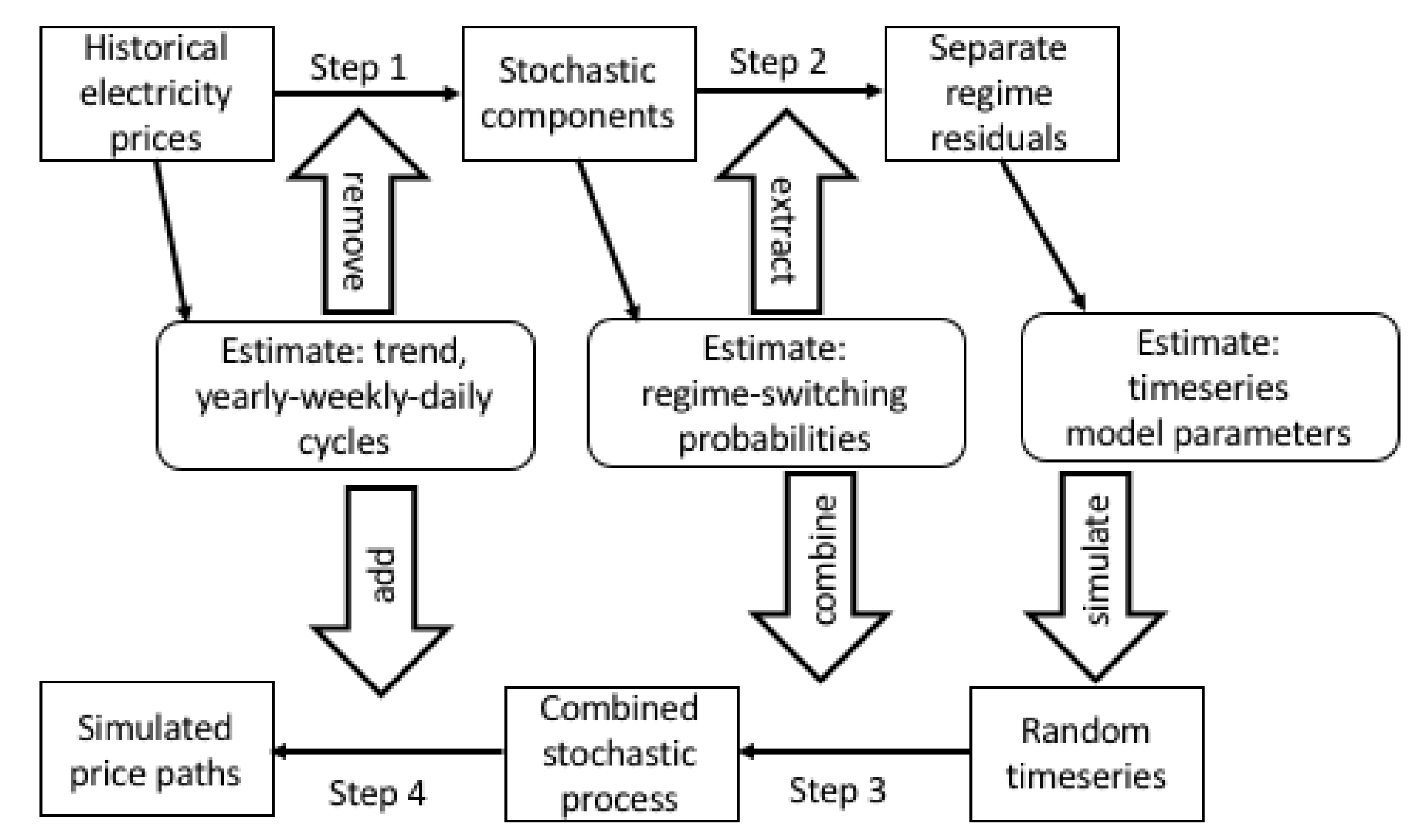
The methodology for price estimation and simulation is represented in Figure 2. The historical price series is used to estimate the deterministic components, namely the trend component and the yearly, weekly, and daily cycles. After the estimation of the deterministic components, they are removed from the historical prices to get the stochastic part in step 1. Then, if a regime-switching model is used, different types of regimes are extracted in step 2. For each regime, the parameters for the time series model are estimated. If a model without regime-switching is used, then step 2 is skipped, and the parameters are estimated from the whole process. The estimated models are used to generate the simulations for the portfolio optimization model described in Section 3.2. First, the random time series are simulated. Then for regime-switching models, the Markov chain is simulated, which changes states according to the transition probability matrix. Then the deterministic components are added in step 4, to get the simulated price processes.

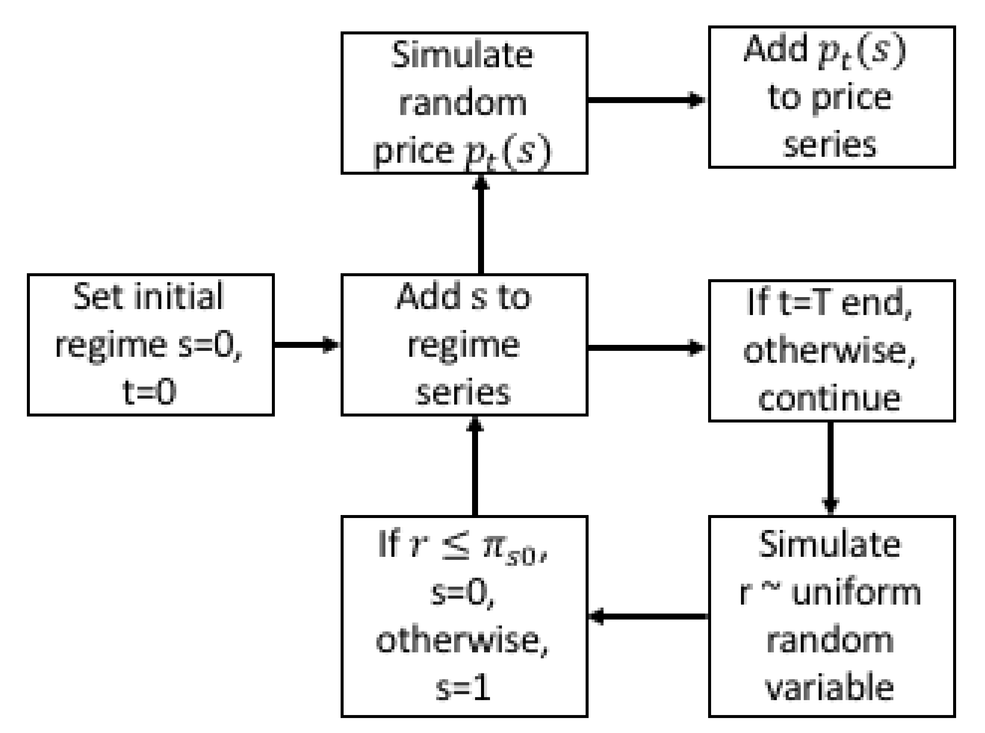
The regime switching models are simulated as shown in Figure 3. In the first step the regime s for time period t is simulated. Then if the regime is regular then the price at time t is simulated using regular process whereas if the regime is jump regime, then the price is simulated using the jump process. A uniform random variable r is used to generate the next period regime. When current regime is regular regime, if r is less than ${\pi }_{00}$, then the regime process at time $t+1$ is also regular regime. Similarly, for a jump regime, if r is less than ${\pi }_{10}$ then the regime is converted to regular regime.

3. Portfolio Risk Management

Extraordinary nature of electricity, i.e., lacking the opportunity of utilizing the inventory, spikes or high weather dependency, makes the market players shape and manage their risk constantly if they want to survive [46]. For example, in the aftermath of the failure of two major plants in the US in 1998, the spot price for electricity have escalated up to USD 7000 per MWatt, noting that the normal price level oscillates in interval of USD 30–60 at that time of the year [47]. In [39], authors compare the relative price volatility of the electricity and some other assets in German spot market on daily scale and concludes that although treasury bills and notes have volatilities less than 0.5% and even very volatile stocks have volatilities around 4% level, for electricity this could go up to 50%. considering that issue, taking action against the extreme spikes in advance would provide the companies from catastrophic outcomes such as bankruptcy.

There is a hypothetical electricity distribution company without any production facilities and the company has to meet the customer demand by buying electricity from producers. Therefore the company faces the risk due to spot price since it is not possible to pass the price fluctuations in the electricity spot market onto customers and price charged to the final consumer is usually fixed. Therefore, the retailer should use risk management tools while making decisions on how to build an electricity purchasing portfolio.

At period $t=0$, assuming an electricity retailer has to decide on how to allocate the portfolio for future electricity delivery for the horizon until time T where $\delta t$ is the price interval (one hour in our case) and there are T periods. The demand is stochastic and equal to $D_t$ at time t and the retailer must satisfy all the demand either by purchasing electricity in the day-ahead market or using available bilateral contracts and derivative markets. Using only the spot market to satisfy demand is very risky because of the high variability of the spot price $X\left(t\right)$ at time t. Therefore, the company can set up different forward contracts indexed by $i=1,2,\cdots ,I$ that are available at the over the counter or the exchange market. The forward contract guarantees delivery of electricity for the given time period and the retailer is obliged to buy the prescribed amount of electricity at the agreed price. Retailer company can decide to buy forward contracts at certain decision times $s\in \mathsf{\Theta }$ where $s<T$ and the coverage period of the contract starts after s. Market price of long position in forward contract i is assumed to be equal to $f^i\left(s\right)$ at time s. Retailer can sell a part of its position on a given contract at a later decision epoch. There are different types of forward contracts, i.e., daily, monthly or quarterly, covering the base period, peak period or the whole period. Peak time forward contract provides a pre-defined amount of electricity between 8:00 and 20:00. Time period between 20:00 and 8:00 are accepted as off-peak time hence the corresponding forward prices are relatively lower than peak hours. Base load contracts supply the consumers some desired amount of electricity 24-hour day time constantly. We define an $I\times T$ indicator matrix $A(i,t)$ as $A(i,t)=1$ if contract i is active at period t and otherwise 0. The volume of contract type i purchased at decision epoch s is denoted by ${\theta }_s^i$. Total amount of electricity contracts that are active at time t are equal to

$$\sum _{i=1}^I\sum _{s\in \mathsf{\Theta }}{\theta }_s^{i}A(i,t).$$

Given the above assumptions, total electricity purchasing costs $C\left(T\right)$ for the period between 0 and T, can be written as given Equation (13).

$$C\left(T\right)=\sum _{i=1}^I\sum _{s\in \mathsf{\Theta }}{\theta }_s^i{f}^i\left(s\right)\sum _{t=1}^{T}A(i,t)+\sum _{t=1}^{T}X\left(t\right)\left(D_t-\sum _{i=1}^I\sum _{s\in \mathsf{\Theta }}{\theta }_s^{i}A(i,t)\right)$$

(13)

Cost function is defined as sum of the cost of purchasing derivative contracts and purchasing extra electricity that is needed. The retailer company does not effect the prices in the market by its decisions.

The objective of the retailer is to minimize $E\left[C\left(T\right)\right]$ with respect to some risk parameter. Different risk definitions are used in the literature and the most widely used risk definition is the variance (or the standard deviation) suggested by [48]. In [48], risk is defined as the variance of returns and a model is given therein for an investor tries to minimize the risk and maximize the return. Following [49] one way to define the risk for electricity retailer company is using the variance of the cost function. Although there has been a well-established research on that risk definition there are some drawbacks require attention. First of all, variance treats the downside risk equal to the upside where the cost is smaller and profits are larger. Furthermore, variance does not satisfy three of the assumptions of coherent risk measures which is discussed at Section 3.2. Although there are possible problems with mean variance models, it is used as a benchmark model at Section 3.1.

An alternative risk definition is conditional value at risk (CVaR). This definition concentrates on the average cost given that the price realisations are at the worst $\alpha$ percentile. Details on this formulation are presented in Section 3.2.

3.1. Mean Variance Model

In line with study given in [49], the goal of the retailer company is to find the portfolio of assets with the minimum expected cost for a predefined level of risk that can be accepted by the company. Risk is defined as the variance of the cost function. Then, purchasing problem of the retailer can be defined as the optimization problem given in Equation (14).

$$\begin{array}{cc}\hfill min& E\left[C\left(T\right)\right]\hfill \\ \hfill \mathrm{s}.\mathrm{t}.& var\left(C\left(T\right)\right)\le {\sigma }_{max}^2\hfill \end{array}$$

(14)

In Equation (14), $var\left(C\left(T\right)\right)$ is the variance of the total costs that the retailer is happy to accept. For mean-variance optimisation problem it is enough to specify the mean and variance of the prices in the electricity spot price series. It is clear from the discussions in Section 2 that the first two moments are not enough to describe the statistical properties of the electricity prices. However, due to the nature of the model the higher moments do not effect the decisions. Therefore, this model is used to see possible drawbacks of the mean-variance formulation.

In this section total electricity demand for the retailer and price of electricity in the spot market are assumed to be independent. This is reasonable since the customers of the retailer use electricity at a constant price. Therefore, their demand structure is not effected by the sudden changes in electricity prices in the market.

Expected cost at time 0 can be written in matrix notation and given in Equation (15).

$$\begin{array}{ccc}\hfill E\left\{C\left(T\right)\right\}& =& \sum _{i=1}^I\sum _{s\in \mathsf{\Theta }}{\theta }_s^i(f^i\left(s\right)-{\mu }_t^p)\sum _{t=1}^{T}A(i,t)+\sum _{t=1}^T{\mu }_t^p{\mu }_t^D\hfill \\ & =& {\theta }^{\prime }\left(1Af-A^{\prime }{\mu }_p\right)+{\left({\mu }^p\right)}^{\prime }{\mu }^D.\hfill \end{array}$$

(15)

In Equation (15), ${\mu }_t^p$ is the expected value of price at time t where ${\mu }^p$ is the vector of means, and ${\mu }_t^D$ is the expected value of demand at time t with ${\mu }^D$ vector. The vectors f consist of price vectors of different derivative contracts for all decision epochs. Similarly, $\theta$ is the decision vector over the quantity bought on all available derivative contracts for all decision epochs. By using the independence assumption, the variance of the cost calculated at time 0 as given in Equation (16).

$$\begin{array}{ccc}\hfill var\left(C\left(T\right)\right)& =& {\theta }^{\prime }{A}^{\prime }{\mathsf{\Lambda }}_{p}A\theta +tr\left({\mathsf{\Lambda }}_p{\mathsf{\Lambda }}_d\right)+{\mu }_p^{\prime }{\mathsf{\Lambda }}_d{\mu }_p\hfill \\ & & +{\mu }_d^{\prime }{\mathsf{\Lambda }}_p{\mu }_d+2{\theta }^{\prime }\left(A^{\prime }{\mu }_p\right)\left({\mu }_d^{\prime }{\mu }_p\right)\hfill \end{array}$$

(16)

In Equation (16), ${\mathsf{\Lambda }}_p$ is the covariance matrix of the prices between different time periods up to 24 periods. Similarly, ${\mathsf{\Lambda }}_d$ is the covariance matrix of the demands between different time periods. Besides, $tr(·)$ is the matrix trace operator. As stated in [49], it is possible to solve this problem using a second order solver.

3.2. CVaR Framework

Value at risk (VaR) is a risk measure used previously in banking industry to calculate the level of possible losses for a portfolio of financial assets. VaR of a portfolio is defined as the threshold level of loss for which the return on portfolio will be greater than that threshold level for $\beta$ percentage of the cases at a given time horizon. Although the main use of VaR is to compute regulatory capital, it has also been used for risk management purposes. The mathematical formulation of $\beta$ percentage value at risk VaR${}_{\beta }$ is

$${\alpha }_{\beta }=min\left\{\alpha \in \Re :\mathsf{\Psi }(x,\alpha ))\ge \beta \right\}$$

(17)

where x is the decision variable and $\mathsf{\Psi }$ is the cumulative distribution function for the random cost depending on x. Since VaR${}_{\beta }$ is a threshold value it is independent of how big the losses can be if the cost is higher than this threshold. The details of coherent risk measures we first introduced in [50]. In contrast to its popularity VaR is clearly not a coherent risk measure since it contradicts the principle of risk reduction by diversification. In addition, it does not provide a convex structure which results computationally intractable optimization models.

An alternative risk measure to VaR is conditional value at risk (CVaR) is defined as the expected value of losses on condition that loss function is greater than VaR threshold. The CVaR formula is given as Equation (18).

$${\phi }_{\beta }\left(x\right)={(1-\beta )}^{-1}\underset{f(x,y)\ge {\alpha }_{\beta }\left(x\right)}{\int }f(x,y)p\left(y\right)dy$$

(18)

In Equation (18), $f(x,y)$ represents a loss function for a random outcome y. CVaR is a coherent and convex measure thus it can be considered as practically more sensible and computationally tractable. Formulation in (18) can be characterised by a convex and continuously differentiable function $F_{\beta }(x,{\alpha }_{\beta })$ in terms of the threshold value $\alpha$ as

$$F_{\beta }(x,\alpha )=\alpha +{(1-\beta )}^{-1}\underset{y\in {\Re }^m}{\int }{\left[f(x,y)-\alpha \right]}^{+}p\left(y\right)dy$$

where ${\phi }_{\beta }\left(x\right)={min}_{\alpha \in R}\left(F_{\beta }(x,{\alpha }_{\beta })\right)$ (for the derivations see [51]). Although the CVaR risk measure provides a convex optimisation problem, evaluation of CVaR efficiently is still intractable. Besides, distribution information of the loss function is often not available. However, one can approximate the risk measure by sampling the probability distribution using samples $\omega$ according to its density function with probability of each sample is equal to ${\pi }^{\omega }$. The resulting approximated function can be written as

$${\tilde{F}}_{\beta }(x,\alpha )=\alpha +\frac{1}{(1-\beta )}\sum _{\omega \in \mathsf{\Omega }}{\pi }^{\omega }{\left[f(x,y^{\omega })-\alpha \right]}^{+}.$$

Since the approximation is a piecewise linear function of the $\alpha$ value, CVaR minimisation problem can be solved using the linear programming technique introduced by [51] through the CVaR constraints using positive auxiliary variables $u^{\omega }$ where $u^{\omega }\ge f(x,y^{\omega })-\alpha$.

In order to convert the electricity retailer cost optimisation problem into CVaR based model, simulation of the price paths are needed. Therefore, the scenario tree based approach as suggested in [52] is used. The sequential simulation method is applied where the nodes are defined as either the decision epochs or the end nodes corresponding to the terminal time. Every node has limited number of leaves and a price path for each leaf is calculated thorough the decision epoch s to $s+1$ using the corresponding process defined as in Section 2. Therefore, each price path from a node to its child node consists of all the simulated prices between times s to $s+1$.

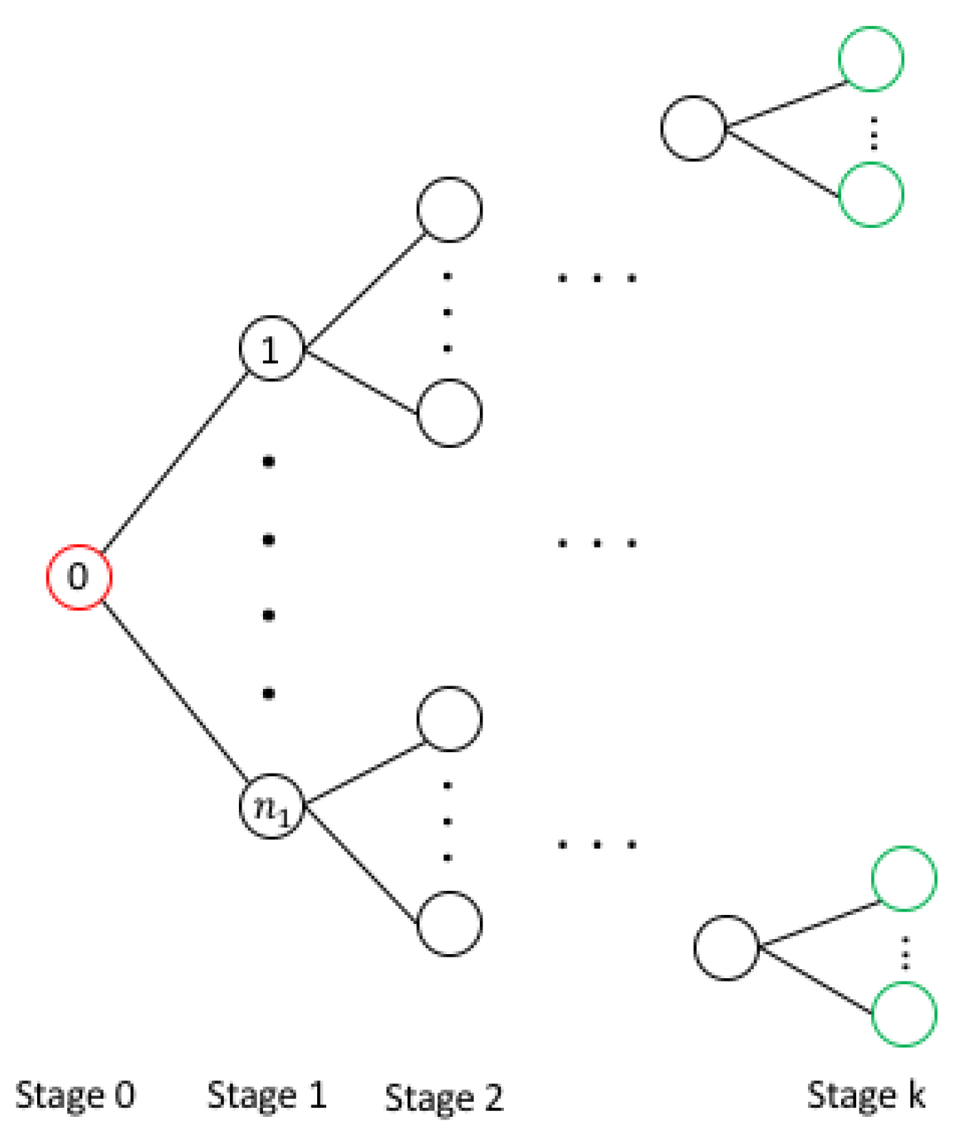
The nodes in the simulation path are defined as follows. The set of all nodes is N including the base node 0 and the set of the terminal nodes $N_K$. A parent of a node n is referred as $pre\left(n\right)$. The time $T_{\left(n\right)}$ refers to the time at which the decisions for node n are taken. The nodes of the decision process is illustrated in Figure 4. The price process has a tree based structure where for each node there are $\overline{n}$ child nodes. In the initial stage there is only one node. Therefore, there is only one decision for this stage initially. This node 0 has $n_1=\overline{n}$ children nodes. Therefore, for all nodes from 1 to $n_1$ the parent node is node 0 ($pre\left(1\right)=pre\left(2\right)=\cdots pre\left(n_1\right)=0$). For stage 1 there are $n_1$ different alternatives. For each possible scenario there is a node that is corresponding to the scenario. Similarly, for each node in stage 1 there are $\overline{n}$ children nodes which results in ${\overline{n}}^2$ total nodes in stage 2. This repeats on subsequent periods; therefore, the total number of nodes at terminal stage (stage k) is equal to $n^k$. In a single stage hedge and hold model the only decision is taken at the initial stage which is represented by a red circle. This approach is compared with a stochastic model. In this case decision is taken at all the nodes except the terminal nodes (green circles). The green circles are the terminal nodes; therefore, no decision is taken at those nodes however the cost is calculated. In this model there are in total $n^k$ possible scenarios however some scenarios follow similar path for some stages; therefore, the tree representation is used. The advantage of the tree representation type modelling is that there no need for nonanticipativity constraints.

One way to use the CVaR formulation is to minimise the risk measure. The portfolio allocation problem with an objective to minimise CVaR risk measure can be modelled as a linear program ($P_{CVaR}$) that is stated as follows:

$$\begin{array}{cc}{P}_{CVaR}:\hfill & \hfill \\ min\hfill & {\displaystyle \alpha +\frac{1}{(1-\beta )}\sum _{n\in N_K}{\pi }^n{u}^n}\hfill \\ \mathrm{s}.\mathrm{t}\hfill & {\displaystyle {\gamma }^n={\gamma }^{pre\left(n\right)}+\sum _{i\in I_n}{\theta }_n^i{f}_n^i\sum _{t=1}^T{A}_{i,t}+}\hfill & \hfill {\displaystyle \sum _{t=T_{\left(pre\right(n\left)\right)}+1}^{T_{\left(n\right)}}{p}_t^n\left(D_t^n-\sum _{i=1}^I{\widehat{\theta }}_{pre\left(n\right)}^i{A}_{i,t}\right)}\\ \hfill & \hfill & \hfill \cdots \forall n\in N/\left\{0\right\}\\ \hfill & {\displaystyle {\widehat{\theta }}_n^i={\widehat{\theta }}_{pre\left(n\right)}^i+{\theta }_n^i}\hfill & \hfill \forall n\in N/\left\{0\right\}\\ \hfill & {\displaystyle u^n\ge {\gamma }^n,u^n\ge 0}\hfill & \hfill \forall n\in N_K\\ \hfill & {\displaystyle {\gamma }^0=\sum _{i=1}^I{\theta }_0^i{f}_0^i\sum _{t=1}^T{A}_{i,t}}\hfill \end{array}$$

In formulation ($P_{CVaR}$), ${\pi }^n$ is the probability of each terminal node. ${\gamma }^n$ refers to the cost of purchasing electricity from market between node $pre\left(n\right)$ and n plus the cost of derivative contracts purchased at time $T_{\left(n\right)}$. Since for node zero there is no parent node, there wont be any electricity price purchased from the market. Similarly at any node $n\in N_K$ it is not possible to buy derivative contracts for the planning horizon; therefore, ${\theta }_{N_K}^i$ are all equal to zero.

In formulation ($P_{CVaR}$), the objective is to minimize the risk. Usually the companies try to find a balance between the risk and return. Decisions taken by merely using risk minimisation models can end up to be too much conservative. As a consequence, the resulting profit would be too small. An alternative formulation can be suggested similar to mean variance problem where the objective is to minimize the expected cost (which results a maximized return) for a given limit on the risk budget. In terms of CVaR framework the intuition is to have a limited budget threshold, and the CVaR of the cost cannot be above which the worst case lost (defined as CVaR). Then the problem turns out to be a constrained portfolio optimisation problem where CVaR value appears as a constraint with a cost minimisation objective. This problem can be formulated as in ($P_{ret}$)

$$\begin{array}{cc}{P}_{ret}:\hfill & \hfill \\ min\hfill & \sum _{n\in N_K}{\pi }^n{\gamma }^n\hfill \\ \hfill & {\displaystyle \alpha +\frac{1}{(1-\beta )}\sum _{n\in N_K}{\pi }^n{u}^n\le B}\hfill \\ \mathrm{s}.\mathrm{t}\hfill & {\displaystyle {\gamma }^n={\gamma }^{pre\left(n\right)}+\sum _{i\in I_n}{\theta }_n^i{f}_n^i\sum _{t=1}^T{A}_{i,t}+}\hfill & \hfill {\displaystyle \sum _{t=T_{\left(pre\right(n\left)\right)}+1}^{T_{\left(n\right)}}{p}_t^n\left(D_t^n-\sum _{i=1}^I{\widehat{\theta }}_{pre\left(n\right)}^i{A}_{i,t}\right)}\\ \hfill & \hfill & \hfill \cdots \forall n\in N/\left\{0\right\}\\ \hfill & {\displaystyle {\widehat{\theta }}_n^i={\widehat{\theta }}_{pre\left(n\right)}^i+{\theta }_n^i}\hfill & \hfill \forall n\in N/\left\{0\right\}\\ \hfill & {\displaystyle u^n\ge {\gamma }^n,u^n\ge 0}\hfill & \hfill \forall n\in N_K\\ \hfill & {\displaystyle {\gamma }^0=\sum _{i=1}^I{\theta }_0^i{f}_0^i\sum _{t=1}^T{A}_{i,t}}\hfill \end{array}$$

CVaR optimization approach takes into account investor’s risk preferences. CVaR minimization and maximization models impose single objective to find an optimal investment strategy. While the first one minimizes risk, the latter maximizes portfolio wealth considering risk preferences of the investor. Multi-objective formulation involves the minimum risk investment strategy to achieve pre-determined wealth $W_{target}$. The size of the problem (in terms of number of constraints and variables) depends on the number of assets as well as the number of scenarios generated. In Section 4 the empirical results of the proposed models is analysed.

4. Computational Experiments

In this section, in order to analyze the effect of different models for the risk management models, a series of experiments are given. Specifically, the objective is to answer the following questions:

• How well different models fit the historical electricity spot price data?
• How do different modeling techniques affect the decisions over derivative contracts?
• How different risk awareness levels of companies affect the total cost of electricity?

In order to address these issues, different models for the electricity spot price are modeled using Python. Then, three different models, the mean-variance model, $P_{CVaR}$, and $P_{ret}$ using simulated price series, are solved. The optimization models are implemented in MATLAB version R2016b using the modeling interface YALMIP [53] and the solver GUROBI version 8.1.1.

4.1. Electricity Price Modelling-Seasonal Part

In the computational experiment part, hourly electricity spot market data between 2012 and 2019 in the Turkish Electricity market is considered. The price data is collected from the EPIAS (Turkish Electricity Market Regulator) website. Descriptive statistics for the entire period and the different years are presented in

Table 1. Descriptive statistics of electricity spot prices (in TRY) in Turkish market.

Period	Average	Standard Deviation	Skewness	Kurtosis
2012–2019	174.729	72.5812	1.85211	29.1861
2012	149.557	61.9412	12.747	334.073
2013	150.081	41.1138	0.197593	10.1976
2014	163.97	33.6955	−0.153973	0.387636
2015	138.011	49.0333	−0.450024	0.348303
2016	140.571	68.8754	4.32308	86.2217
2017	163.844	39.0925	0.756796	19.9034
2018	231.636	72.1105	0.174506	−0.627248
2019	260.32	83.9872	−1.65767	2.00645

. The historical data show that the electricity spot market has very heavy tails and positively skewed. This situation verifies the non-normality of the data and the need for the use of extreme jumps. Furthermore, the averages tend to change from one year to another, where the most noticeable change occurred from 2017 to 2018. The reason for this case is the rapid increase in exchange rates in Turkey. Due to the increase in exchange rates, electricity prices have also increased since a significant portion of Turkey’s production depends on imported resources, such as natural gas.

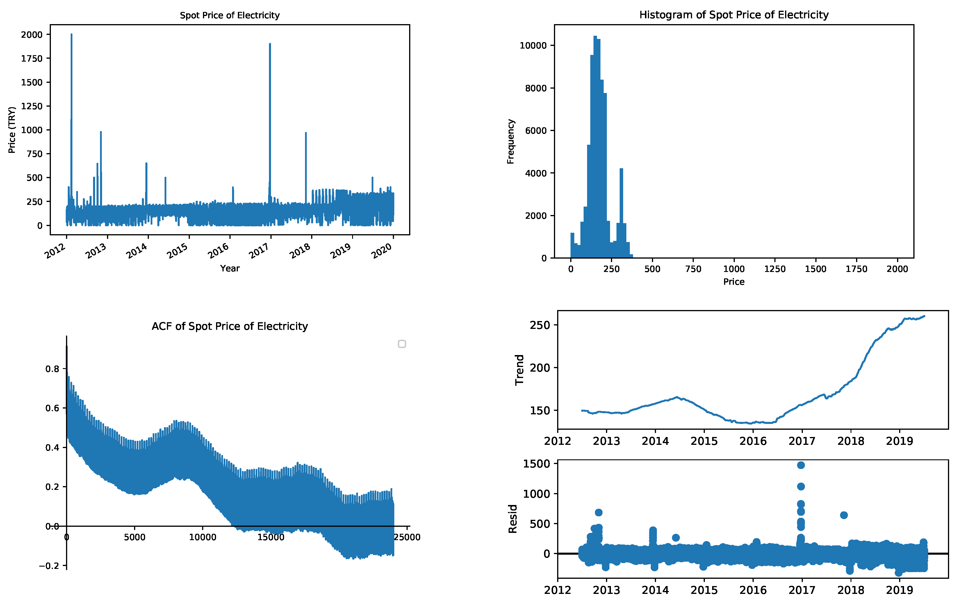
If the historical spot prices are analyzed, the jumps are evident. Figure 5 displays the historical prices from 2012–2019 in the top-left chart. The highest allowable price in Turkey is 2000 Turkish Liras. The jumps are more common in the year 2012, which can also be observed by the skewness and kurtosis values in Table 1. However, in the years 2014 and 2015, they are smoother. The top-right chart represents the histogram of the prices. The nonnormality and the two-state pattern of the prices are observable in the histogram. The bottom-left chart of Figure 1 shows the corresponding autocorrelation function (ACF), which clearly shows the price data’s seasonal behavior. The autocorrelation function plot is for lags up to 24,000 h. Here the weekly seasonality can be observed with small stings, whereas the sinusoidal shape shows the yearly seasonality.

The spot price has a positive trend component, which can be observed by comparing the yearly averages in Table 1. The trend component can be removed by decomposition analysis in the time series. Trend component, calculated by taking the yearly average values, is given in the bottom-right chart of Figure 5. The trend is smooth around 150 TRY until 2016 and increases steadily after that point as the exchange rates against Turkish Lira rise.

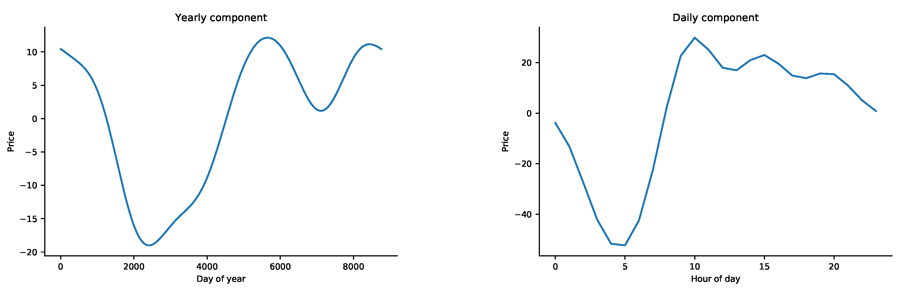
The yearly seasonal component is derived through Equation (2) using the de-trended data for $k=5$. The parameters for the yearly component are summarised in

Table 2. Yearly and daily components.

	${\mathit{\beta }}_1$	${\mathit{\phi }}_1$	${\mathit{\beta }}_2$	${\mathit{\phi }}_2$	${\mathit{\beta }}_3$	${\mathit{\phi }}_3$	${\mathit{\beta }}_4$	${\mathit{\phi }}_4$	${\mathit{\beta }}_5$	${\mathit{\phi }}_5$
Yearly Trend	12.04	0.82	7.93	0.07	1.86	1.00	−1.42	0.01	0.97	0.33
Daily Trend	−30.27	0.14	−16.98	0.68	8.17	0.04	−3.83	0.24	2.20	0.01

. The $\phi$ values represent the time in terms of years in the yearly component row. For example first component has width of ${\beta }_1^y$= 12.4 where the top point is at ${\phi }_1^y$ = 0.82 years which is around end of October. The weekly components are calculated using regression, and the value of price for each day compared to the average price is given in

Table 3. Weekly components.

Period	Monday	Tuesday	Wednesday	Thursday	Friday	Saturday	Sunday
$W_i\left(t\right)$	1.653	3.193	3.531	3.822	3.554	−1.274	−14.45

. The parameters for the daily component are also given in Table 2, where the $\phi$ values represent the time in terms of days for this case. The yearly and daily seasonal component functions are given in Figure 6.

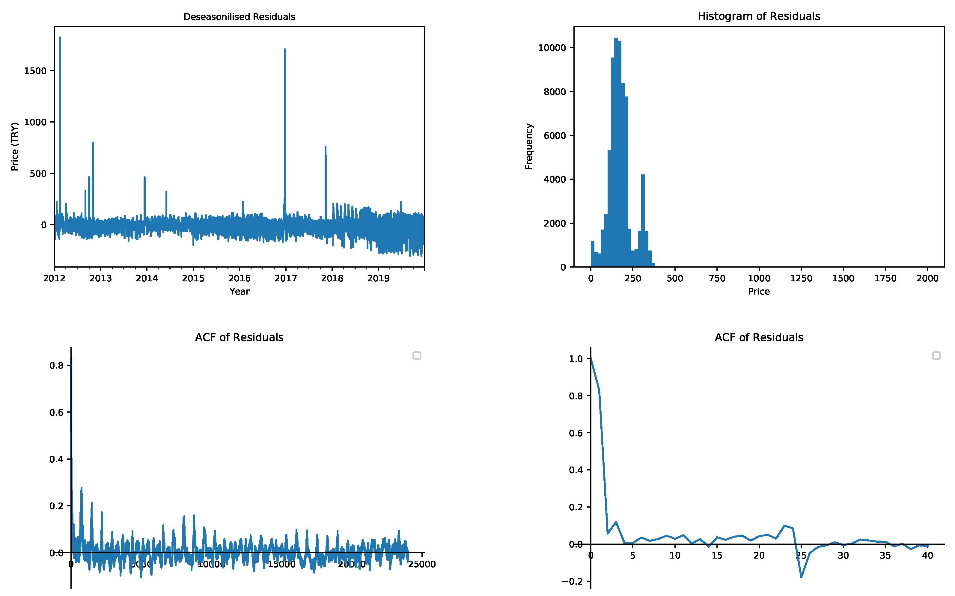
The residuals are derived after cleaning all the seasonal and trend components. Figure 7 presents the histogram, the autocorrelation function, and the partial autocorrelation (PACF) for the residual process. From the PACF diagram, one can observe the autoregressive behavior. When tested for unit root using Augmented Dickey–Fuller test, the null hypothesis of series possessing a unit root is rejected with a p-value less than 0.0000001 and it is strongly shown that the data does not have a unit root. Therefore, both the ARMA models and the mean reversion model can be used. Residuals are used to model the processes that are introduced in Section 2.

4.2. Electricity Price Modelling-Stochastic Part

The processes that are introduced in Section 2 are used to model the residuals after removing the trend and seasonality components. The models used are; mean reversion process, ARMA process, and GARCH process. Three different ARMA models are selected according to their Bayesian information criterion (BIC) values. The GARCH model is driven for the ARMA(1,1) model. The parameters for different types of models estimated for dates between 2012 and 2019 are shown in

Table 4. Model parameters.

	Models
Parameter	MR	ARMA(1,1)	ARMA(5,1)	ARMA(6,3)	GARCH(1,1)
$\mu$	-	−0.0071	0.097	0.0013	−0.3715
$\sigma$	0.312	-	27.873	27.721	-
$\kappa$	0.829	-	-	-	-
${\alpha }_1$	-	0.8584	1.711	0.725	0.0839
${\alpha }_2$	-	-	−0.765	−0.048	-
${\alpha }_3$	-	-	0.148	1.061	-
${\alpha }_4$	-	-	−0.128	−0.726	-
${\alpha }_5$	-	-	0.030	0.045	-
${\alpha }_6$	-	-	-	−0.067	-
${\beta }_1$	-	0.8584	−0.948	0.043	0.9039
${\beta }_2$	-	-	-	0.041	-
${\beta }_3$	-	-	-	−0.946	-
GARCH- $\omega$	-	-	-	-	11.8629

. A jump or state change is defined as the cases where the residual is at least three standard deviations different from the mean. The mean reversion with jump process has the jump probability equal to $1.28\%$ with an average jump size of $151.7$ from the seasonal expected value. The parameters for regime-switching models are estimated by separating the base regime and jump regime. Here the probability that the next hour will be a base regime given this hour is a base regime is ${\pi }_{00}=0.977$, whereas the next hour will be a peak regime given this hour is a peak regime is ${\pi }_{11}=0.769$. This shows that disruptions in average continues for 4.32 h.

After estimating parameters for each model, predictive performances of the simulations are evaluated. Three error measures are selected: mean average percentage value (MAPE), root mean squared error (RMSE) and coefficient of determination ($R^2$). The formulae of these performance measures are given in Equations (19) and (20). In these equations, N, T, and P represents the number of simulations, the number of simulated hours and the prices, respectively.

$$E\left(MAPE\right)=\frac{1}{N}\sum _{k=1}^N\frac{1}{T}\sum _{t=1}^T\frac{\left|P_{k,t,generic}-P_t\right|}{P_t}$$

(19)

$$E\left(RMSE\right)=\frac{1}{N}\sum _{k=1}^N\left(\frac{1}{T}\sqrt{{\sum }_{t=1}^T{\left(P_{k,t,generic}\right)}^2)-P_t}\right)$$

(20)

The calculations are done through sorted price paths of both the historical data and the simulated data. The reason to use sorted paths is that the retailer is not concerned about exactly knowing when the price jump will occur but it is more interested in the number and amplitude of the jumps. A sorted comparison gives a better measurement on how well each model works over modelling the jump processes. The sorted price paths are called price duration curves. In order to achieve robust results we determine the quality of solutions over 100 simulated paths for every model. The results of performances for different models used are given in

Table 5. Error measures of different models between 2012 and 2019.

MODEL	RMSE	MAPE	${\mathit{R}}^2$
ARMA(1,1) w/o RS	11.58	28.80	0.74
ARMA(1,1)-GARCH(1,1)	12.45	28.70	0.74
ARMA(5,1) w/o RS	14.76	29.67	0.74
ARMA(6,3) w/o RS	10.98	29.04	0.78
Mean Reverting W/o RS	9.09	34.55	0.88
Mean Reverting- Jump process	8.49	21.14	0.81
ARMA(1,1) w/RS	6.95	19.17	0.88
ARMA(5,1) w/RS	7.37	21.98	0.88
ARMA(6,3) w/RS	7.34	28.19	0.85
MR w/RS	6.54	27.01	0.93

. It is clear that the regime switching models perform better in terms of $R^2$ and RMSE criteria. This shows the importance and advantage of using models with regime switching.

4.3. Hedging Portfolios

In this section, the results for different portfolio hedging problems are presented, particularly mean-variance, $P_{CVaR}$, and $P_{ret}$. Different models for spot price processes are assumed and the price paths according to those processes are simulated. The objective is to compare the goodness of fit results calculated in Section 4.2 with hedging performance results.

Demand forecast is assumed as 5% of total demand of electricity market in Turkey for the retailer. The planning horizon is assumed to be three months. Two different planning scenarios are analysed, in particular

• The only decision epoch is the beginning of three month period;
• There are three different decision epochs at the beginning of each month in the decision quarter.

Therefore, in the first plan the decision maker builds his/her hedging portfolio initially then does not buy or sell any more future/forward contracts. In the second scenario the decision maker can update his/her portfolio at intermediate time periods. The price paths are simulated as a tree type structure where the nodes are placed at the decision points and each node has 20 children which results in a total of 8000 scenarios. For each experiment 10 replications are performed.

In the market there are monthly and quarterly contracts for peak, off peak and base hour of electricity. The peak contract is sold at a 3% premium compared to the expected cost of electricity. The off peak is sold at par and the base contract is sold at 1% premium. These are parallel with the real market conditions.

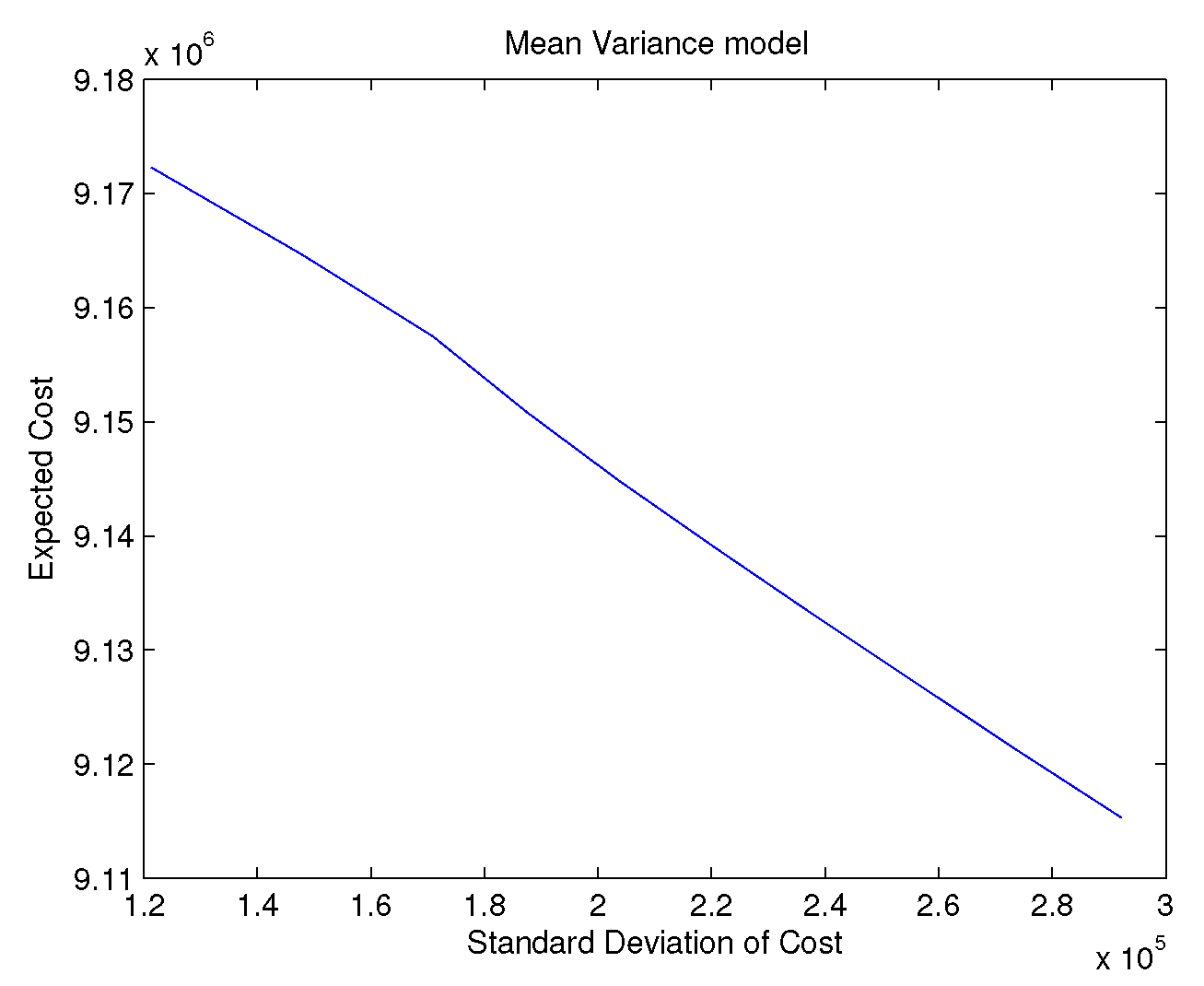
For the mean-variance case the historical data is used to calculate the mean vector and covariance matrix. In Figure 8 we present the results for mean variance model at different levels of variance tolerance. The efficient frontier is different from the portfolio optimisation case since the objective in our problem is to minimise cost rather than maximize the profit.

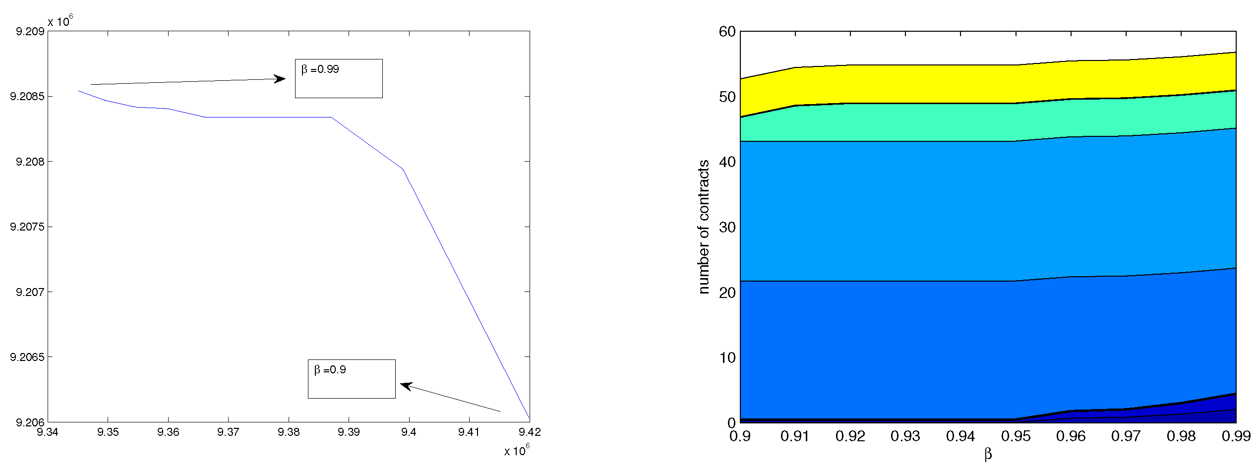
Figure 9 presents the results for simulations done using ARMA(1,1) in model $P_{CVaR}$ with decisions made at the beginning. Here, as the $\beta$ value increases the risk appetite of the retailer company decreases so the number of contracts that are purchased increases. Furthermore, the expected cost increases. The CVaR values are the empirical $95\%$ CVaR of simulated results. Furthermore, the area plot shows how many of each derivative the retailer buys at given levels of $\alpha$.

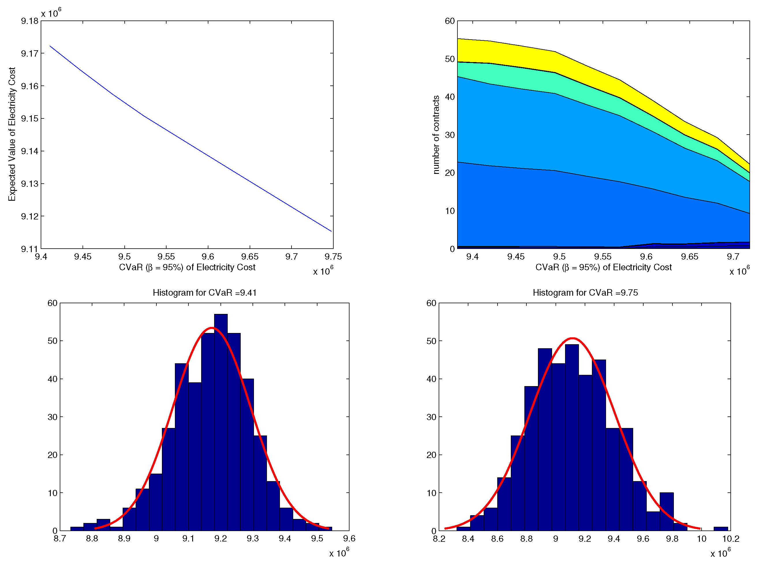
Figure 10 presents the solutions for model $P_{ret}$ and where the simulations are done using ARMA(1,1) with decisions made at the beginning. Here $\beta =95\%$ and the budget level i set between the optimal solution of $P_{CVaR}$ and the budget needed if no derivative contract is bought. It can be observed that the number of contract needed increases with the increased budget. Furthermore, the contract mix does not change as the budget is increased. A higher budget allows the retailer to minimise the expected cost. The histograms shows the results of scenarios with respect to different budget levels. The diagram on the left shows the cost scenarios for a budget of 9.41 M whereas the one on the right shows the scenario results for a budget of 9.75 M. If the budget is tight more contracts are bought so it is less likely that very high costs are seen. But also low costs are not possible.

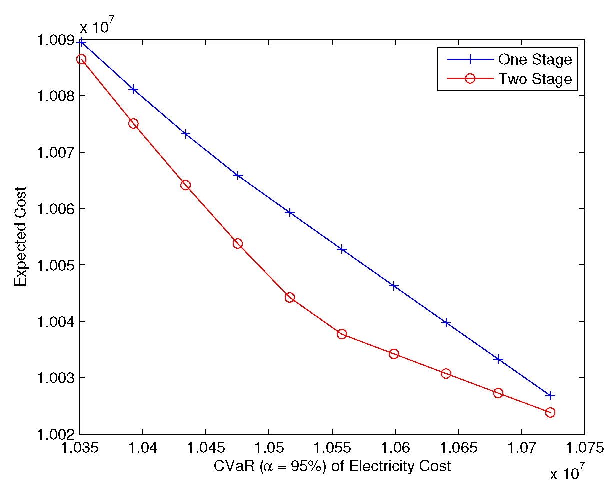
In order to compare multi-stage decision making with the hedge and forget approach the expected cost and CVaR values for two models in Figure 11 are compared using different budget levels. The stochastic programming approach provides lower cost or lower risk because if in the first period there are not too many jumps then the budget available and the company hedges only small part of portfolio. If there were a lot of jumps then company needs to buy more contracts to hedge in the remaining periods.

In order to compare different models an out-sample analysis is performed. First the parameters are estimated using 2012–2015 data. Then the electricity prices are forecasted for each quarter as a rolling horizon. In

Table 6. Out-of-sample error measures and electricity purchase cost

MODEL	RMSE	MAPE	${\mathit{R}}^2$	Average Cost
ARMA(1,1) w/o RS	16.02	29.66	0.60	9.74
ARMA(1,1)-Garch(1,1)	15.68	29.36	0.59	9.71
ARMA(5,1) w/o RS	18.13	34.68	0.65	9.76
ARMA(6,3) w/o RS	14.42	35.61	0.78	9.57
Mean Reverting W/o RS	12.77	37.17	0.85	9.56
Mean Reverting- Jump process	12.82	27.59	0.76	9.58
ARMA(1,1) w/RS	10.31	24.09	0.78	9.56
ARMA(5,1) w/RS	10.62	24.53	0.76	9.58
ARMA(6,3) w/RS	9.75	32.61	0.83	9.49
MR w/RS	11.56	27.43	0.87	9.44

the out of sample error measures estimated for each of the 4 quarters using different models are summarised. Furthermore, the cost of electricity purchase using $P_{CVaR}$ case with three stage recourse for every model is presented. It is clear that the regime switching models behave better compared to standard models. This also shows that using regime switching can better explain the electricity spot price data and also can be useful for risk management applications.

5. Conclusions

In this paper, the hedging portfolio allocation problem for an electricity retailer company under the price uncertainty is studied. The retail companies that operate in this market may either buy the electricity at the day ahead market or hedge their electricity price risks via bilateral contracts or financial derivative instruments. Since the bilateral agreements depend on the private negotiations between different parties, the derivative contracts are used. The company aims to hedge its cost of electricity for a given period. The company’s objective is either minimization of the risk of cost or minimization of the cost of electricity for a given level of the risk level. For this setting, a multi-stage stochastic optimization model that decides on the monthly and quarterly hedging strategies is developed.

The risk is defined as the CVaR for the cost in addition to the variance of the cost. In order to calculate CVaR values, price scenarios for electricity are generated. The electricity prices bear highly volatile properties due to unexpected jumps. Therefore, appropriate models are needed. The Electricity price paths are simulated through different stochastic processes. The standard models and their extended counterparts with their regime-switching components, which can capture the jump phenomenon, are analyzed. It is observed that using the regime-switching approach not only fits the data better for an in-sample experiment but also has better forecasting power at the out-of-sample analysis. Therefore, we conclude that regime-switching models have the power to capture structural changes that result in instantaneous jumps in the prices. As a result, the use of complex models that incorporate Markovian structure is inevitable for the players in the electricity market for price simulations.

This paper’s main contribution is to combine the price forecasting and model comparison part with the risk management problem. Computational tests are conducted by using datasets for the Turkish electricity market regulated by Epiaş. The portfolio optimization and risk hedging properties of different models are compared according to their performances in the conditional value at risk problems. In particular, for the out-of-sample examination, comparison in terms of risk levels for various models is carried out and added as an extra column in addition to the forecasting metrics in the results table. For the in-sample analysis, best models appear to be ARMA(1,1) with regime-switching and mean reversion with regime-switching according to RMSE and MAPE values. For the out-of-sample analysis, regime-switching models behave better according to both the forecasting metrics and financial performances. The regime-switching models have around 1% lower cost compared to their standard counterparts. The model with the lowest cost after hedging is mean reversion with regime-switching. This result shows that if a model to capture the jump component such as a Markovian process is used, then even with simple models, it is possible to achieve good hedging performance. Since the regime-switching models perform better than their traditional counterparts, a market participant in the electricity sector is advised to use Markov processes in their scenario generation models.

Another contribution of this study is the modeling and analysis of multi-stage risk models. A scenario tree for electricity price simulations is generated. In the computational experiment section, a quarterly planning horizon with monthly balancing decision epochs is analyzed as an alternative to the hedge-and-wait approach. A multi-stage CVaR optimization model where the portfolio is managed dynamically is modeled and solved in this paper. It has empirically been shown that the multi-stage model results in better portfolios in terms of risk and profit. The Pareto optimal solutions for the dynamic case results in a more efficient frontier compared to the static case where all decisions are taken upfront with a risk reduction of around 2.5% for the same level of cost. Therefore, a multi-stage CVaR model, as the methods introduced in this paper, which can hedge the price risks in the market dynamically, is inevitable for the electricity distribution companies.

We conclude that the risk-averse approaches for electricity distribution companies can decrease the company’s price risk through a slight increase in cost. Proper model selection for the price before the optimization step remarkably increases the benefit of the model. In particular, the regime-switching approaches to capture the jumps in the electricity prices are markedly lucrative.