Two-Stage Fuzzy Logic Inference Algorithm for Maximizing the Quality of Performance under the Operational Constraints of Power Grid in Electric Vehicle Parking Lots

Abstract

The widespread adoption of electric vehicles (EVs) has entailed the need for the parking lot operators to satisfy the charging and discharging requirements of all the EV owners during their parking duration. Meanwhile, the operational constraints of the power grids limit the amount of simultaneous charging and discharging of all EVs. This affects the EV owner’s quality of experience (QoE) and thereby reducing the quality of performance (QoP) for the parking lot operators. The QoE represents a certain percentage of the EV battery required for its next trip distance; whereas, the QoP refers to the ratio of EVs with satisfied QoE to the total number of EVs during the operational hours of the parking lot. This paper proposes a two-stage fuzzy logic inference based algorithm (TSFLIA) to schedule the charging and discharging operations of EVs in such a way that maximizes the QoP for the parking lot operators under the operational constraints of the power grid. The first stage fuzzy inference system (FIS) of TSFLIA is modeled based on the real-time arrival and departure probability density functions in order to calculate the aggregated charging and discharging energies of EVs according to their next trip distances. The second stage FIS evaluates several dynamic and uncertain input parameters from the electric grid and from EVs to distribute the aggregated energy among the EVs by controlling their charging and discharging operations through preference variables. The feasibility and effectiveness of the proposed algorithm are demonstrated through the IEEE 34-node distribution system.

1. Introduction

The shortage of fossil fuel in the world and the concerns about the negative impact of conventional vehicles on the environment have raised attention towards exploring alternative energy sources for transportation. One of the possible solutions to tackle such problems is to replace conventional vehicles with electric vehicles (EVs). As a result, widespread adoption of EVs will be observed in the near future. For instance, the global stock of EVs has been estimated to be about 40–70 million by 2025, and more than one hundred million EVs by the year 2050 [1,2]. These EVs are moving across cities and have the potential to serve the power grid through charging and discharging with the availability of vehicle-to-grid (V2G) technology.

The integration of large-scale EVs into the electric grid requires a specific and costly infrastructure. On the other hand, parking lots (PLs) are alternative solutions that can help to efficiently utilize the potential of EVs within the existing power system [3]. PLs are regarded as a platform where the aggregated EVs represent the electric load as well as the power supply resources for the electric grid in grid-to-vehicle (G2V) and vehicle-to-grid (V2G) mode, respectively [4]. As the EVs are staying for a longer period of time, therefore; in G2V mode, their charging load may coincide with the baseload (residential load). In [5] the authors identified an overlap between vehicles on the street and the residential load profile from 2:00 p.m. to 6:00 p.m. An uncontrolled simultaneous charging of a fleet of EVs during such an overlap time may greatly stress the distribution power network in terms of power losses, voltage fluctuations, degraded power quality and efficiency which may increase the chances of a power blackout. The possible reasons for such a huge load are the simultaneous charging of a large-scale EVs and their use of fast charging stations (CSs).

Most of the global companies under the international coalition initiative (EV100) commitments are transitioning their internal combustion engine vehicle parks into EV parks with fast CSs. For instance, Tesla has already announced a plan to build supercharging stations, where 50 stations have been installed in Shanghai and others in Beijing and the USA [6]. In V2G mode, simultaneous discharging of such a large scale of EVs is not a desirable solution from both the power grid and from the EV owner’s perspective. Therefore, the PL operators are required to limit the charging EVs during the peak-hours and the discharging EVs during the off-peak hours. However, on the other side, this can have a significant effect on the desired quality of experience (QoE) level for the EV owners during their parking duration. This implies that PL operators are expected to satisfy the QoE for a maximum number of EVs and thereby to improve the PL quality of performance (QoP). Considering 12 h as the parking operational hours, a higher value of QoP in a day corresponds to better performance and vice versa. Therefore, selection of the most appropriate EVs for charging and discharging services among all the EVs candidates such that to maximize the QoP while respecting all the operational limits of the power grid is a complex problem. The complexity of this problem is due to the dependency of the QoE satisfaction level on multiple and independent factors, including the arrival time, departure time, parking duration, state-of-charge (SoC), next trip travelling distance, required SoC (SoC^req), the current PL occupancy and the updated available power from the grid. These are temporal and spatial based varying parameters with a higher level of uncertainty and thereby resulting in a dynamic and complex system. In practice, the drivers and the PL operators perceptions on several of the above parameters are highly imprecise. For instance, the driver’s description of SoC is likely to be non-specific and qualitative, for instance: enough, low or high. Similarly, the postulation of PL operators about the available power is simply as low, medium or high. In order to efficiently utilize the energy usage, the scheduling of charging and discharging of EVs can play an important role and should consider the aforementioned factors from both the power grid and EV domains. However, the uncertain behavior of EV owners and the requirements of both EVs and of the power grid present challenges for the PL operators to efficiently schedule EVs operation and thus affecting their QoP.

One of the possible solutions to deal with such types of temporal and spatial varying complex systems is to apply a fuzzy logic-based methodology. The fuzzy-logic based approach resolves the nonlinearity of any real-time complex system by breaking it down into a simple weighted sum of linear subsystems [7,8]. The growing trend of EVs, the owner’s parking behavior, charging and discharging requirements, the electric power grid constraints, and the fuzzy approach towards solving such complex systems motivated us to develop a scheduling algorithm based on two-stage fuzzy logic inference system for EV PLs. The TSFLIA takes the flexibility of EV owner’s behaviors into account and aims to schedule the charging and discharging operations for the most appropriate EVs such that it helps to maximize the QoP under the operational limits of the power grid. To do so, the TSFLIA utilizes the services of the developed first and second stages of the fuzzy inference mechanisms for computing the required SoC of EVs according to their next trip travelling distance and schedule their charging and discharging operations under the smart grid operational limits. The input parameters such as the departure time from home arrival time to PL departure time from PL, required SoC, parking duration and the available power for controlling the charging and discharging operation of EVs are believed to be adequately accurate for solving this complex problem. The proposed scheme is validated using the IEEE 34-node distribution system and simulated for three different PLs. The simulation results indicate that the QoP with the proposed TSFLIA prevails over the fuzzy logic inference based algorithm (FLIA) for electric vehicles in PLs. The contributions of this research work are as follows:

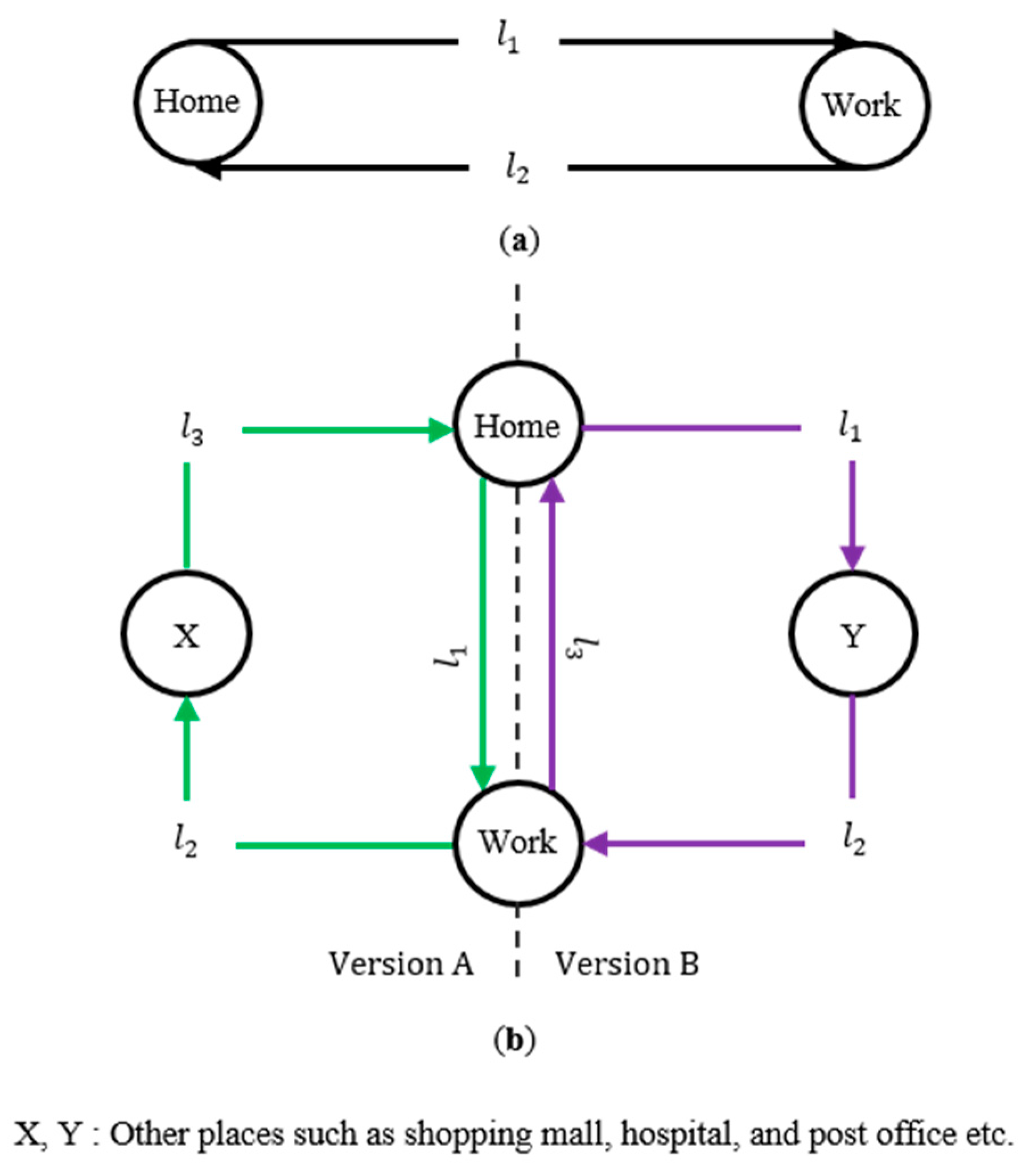
• The energy requirements of the EV owners are identified using realistic traveling distance patterns from the US national household travel survey (NHTS) and their G2V and V2G operations are formulated and solved through a TSFLIA.
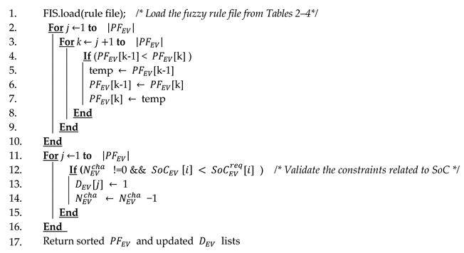
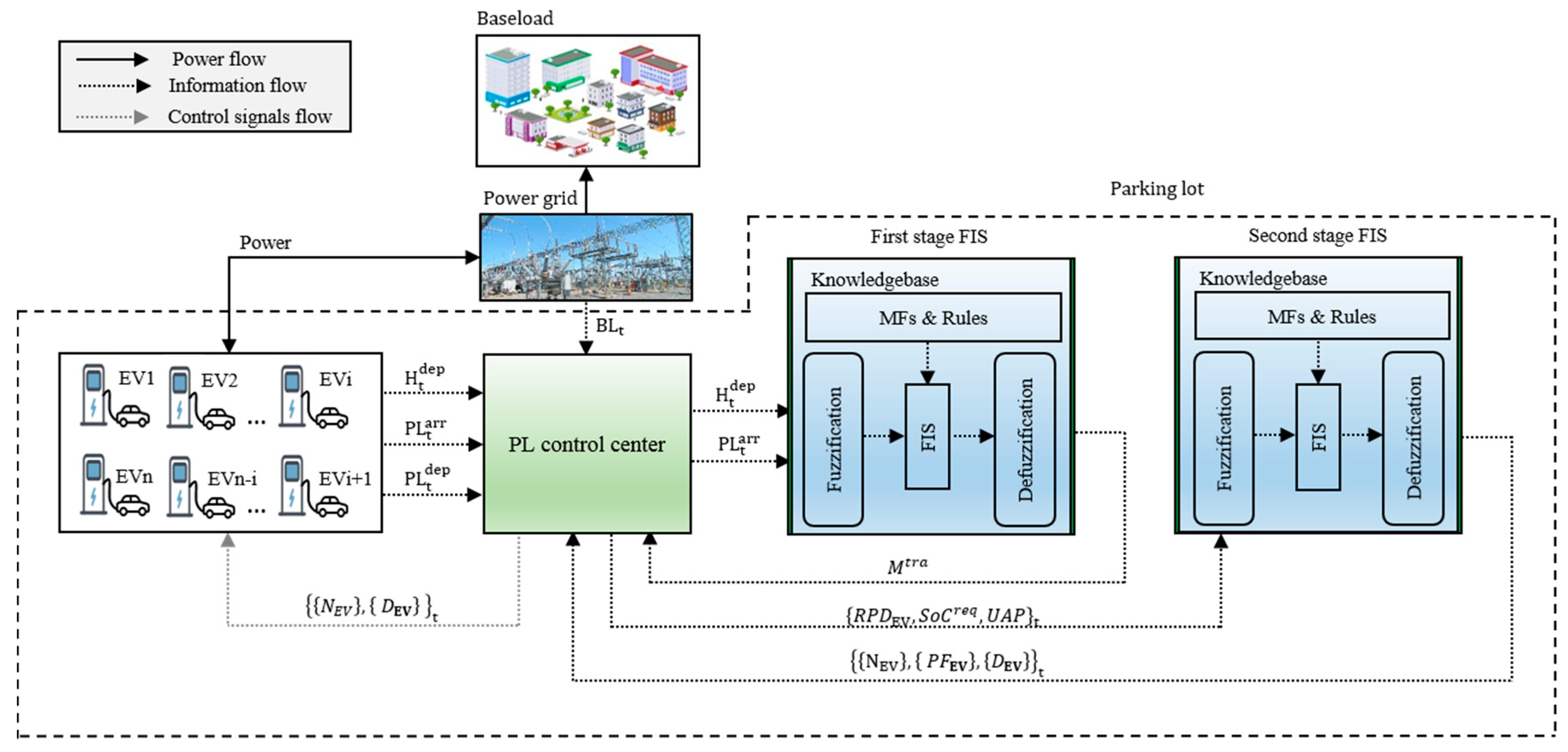
• The first stage fuzzy inference system (FIS) is developed based on the real data obtained from the NHTS to compute the aggregated charging and discharging energies of EVs according to their next trip travelling distances. The second stage FIS utilizes the inputs from EVs and the power grid to determine an adequately accurate charging and discharging preferences for each of the connected EVs.
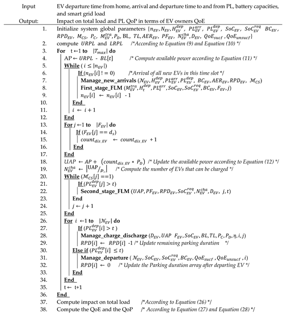
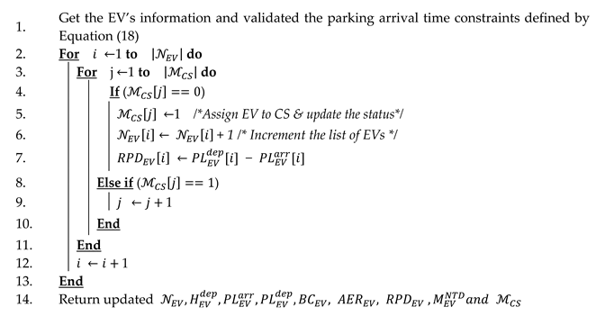
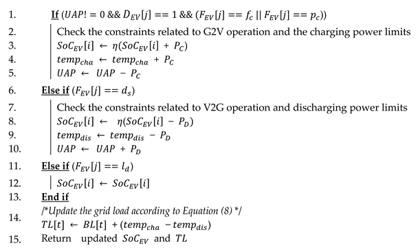
• The TSFLIA is developed with five sub-algorithms: (1) Manage_new_arrival, (2) First_stage_FLM (Fuzzy Logic Module), (3) Second_stage_FLM, (4) Manage_charge_discharge, and (5) Manage_departure. The registration of new arriving EVs, the departure of served EVs and the maintenance of PL occupancies are serviced by Manage_new_arrival and Manage_departure. The First_stage_FLM resolves the departure time from home and arrival time to PL to compute the SoC and required SoC of EVs according to their traveled and next trip distances and categorizes the operation of EVs in G2V, V2G and idle modes. The Second_stage_FLM account an accurate preference for each of the connected EVs by comprehensively solving the complexity of temporal based varying available power, required SoC for the next trip and EVs remaining parking duration. In each sampling period, the scheduled G2V and V2G operations of EVs are controlled according to their preference values through the sub-algorithm Manage_charge_discharge.
• The proposed TSFLIA is applied to three different PLs connected to the IEEE 34-node distribution system and the results are validated against the FLIA.

The paper is organized as follows: Section 2 explores the state-of-the-art techniques in this area. In Section 3, the proposed TSFLIA is presented. The simulation environment and results are discussed in Section 4. Finally, the paper is concluded in Section 5.

2. Related Work

In the literature, the problem of scheduling EVs for future smart PLs has been extensively studied with different perspectives and objectives. This includes power allocation to PLs, energy and cost management of PLs, PLs placement in the power distribution network and routing and PL selection for moving EVs. A scheduling algorithm for EVs based on fuzzy logic control with the aim to reduce the waiting time for charging and balance the charging load of EVs was proposed in Ref. [9]. The developed fuzzy logic control system was used to compute a weighted priority for each of the EVs and CSs and determine their optimal pairs. By this way, they evenly distributed the charging load of EVs among the available CSs for reducing the waiting time. The performance of the proposed scheme was analyzed through average waiting time and was compared with the conventional random and maximum weight-based scheduling schemes. However, the authors only focused on the waiting time requirements of the EV owners while they did not address the charging level satisfaction and optimization of energy consumption.

The authors in [10] proposed a multi-agent scheme for the rerouting of moving EVs towards the appropriate CSs with the aim to distribute the charging load among the dispersed CSs. The multi-agent scheme was built in a bottom-up hierarchical manner where each agent was modeled with different services. An EV agent was modeled based on a fuzzy logic expert system which was used to request the other high-level agents for charging and discharging services. A case study was conducted by considering 21 EVs with battery capacities of 100 kWh and 6 CSs dispersed within a virtual block to validate their proposed scheme. The results indicate that the proposed scheme was able to cognitively redistribute the EVs among the CSs. However, the work focused on the distribution of the preload of EVs (i.e., the load at the time of request) and did not consider the situation of already parked EVs. The authors in [11] considered the mobility of EVs and studied the problem of analyzing the impact of different sampling rates on the communication channel with the G2V and V2G operations of EVs. The authors concluded that a faster sampling data rate between the three communicating entities (i.e., aggregator, EVs and CSs) can help in reducing the error. However, the work mainly focused on the sampling rate of requests and the impact on the communication channel instead of any scheduling for EVs or optimization of the power grid load.

A G2V and V2G capabilities for voltage stability and mitigating peak demand in a typical power distribution were studied in [12]. Two controllers were designed: one for CS and another for the aggregator to control the V2G operation based on fuzzy logic. The CS controller was used to determine the output charging and discharging energy according to the SoC of EVs and voltage of the nodes. The output of the first fuzzy controller coupled to the node voltage was used as inputs to the second controller which results in power flow between the nodes with connected CSs. The simulation results demonstrated that the G2V and V2G operations were controlled efficiently while using a fuzzy logic controller. However, the authors did not consider the QoE requirements of the EV owners. An integrated G2V and V2G scheme based on fuzzy logic and genetic algorithm (GA) was developed to maximize the penetration of EVs in a workplace car park [13]. The developed fuzzy logic inference system used two inputs: the SoC and subsequent trip distance (STD) to compute a weighted value for decision. For each of the EVs, the fuzzy logic inference was returning two outputs: one for charging while the other for discharging. The two output values were compared to determine the charging and discharging status of each the EVs. After the status determination of each EV, the G2V and V2G operations were scheduled using GA. The results of the proposed scheme showed maximum penetration of EVs with reduced cost in industrial and commercial laterals of the 38-node distribution system. The authors in [14] proposed a probabilistic approach for determining optimal locations for EV PLs in the distribution network by considering driving patterns of EVs owners and scheduled the charging and discharging of EVs based on the electricity prices. The authors concluded that minimizing the difference between the initial and final SoC of EVs, or in other words, satisfying the charging and discharging requirements of a maximum number of EVs could increase the benefits for the PLs. However, the problem of minimizing the differences between initial and final SoCs still needs to be explored, because there are multiple factors such as arrival and departure time of EVs, initial SoCs, battery capacities, charging and discharging rate, and the available power which influences the operations of PLs.

A real-time charging scheme based on fuzzy logic inference was proposed in [15] with the aim to manage the aggregated charging load and satisfies the EVs in a fair manner. The developed fuzzy inference system was used to determine the charging or discharging priority value based on the associated inputs such as remaining charging time, the SoC and the electricity price. Given the priority value, an optimization model using linear programming (LP) was adopted to obtain an optimal charging or discharging rate for each EV. Two different cases with discharging only and charging and discharging were simulated to validate the proposed scheme. However, the proposed scheme assumed that the V2G operation was based on the willingness of EV owner’s regardless of their requirements. Therefore, the rationality of their participation in V2G operation and their required amount of charge/discharge are yet to be exploited. An online decision-making scheme for managing the charging loads of plugged-in electric vehicles (PEVs) in public PLs was proposed for aggregators [16]. In their scheme, a fuzzy expert system was used to assign a charging priority value to each EV by evaluating the required SoC, maximum charging rate, and parking duration for making a decision. The optimization problem was then formulated using mixed-integer nonlinear programming and the proposed method was applied on a 38-node distribution network. The proposed scheme addressed both the requirements of the power grid and the EV owner’s QoE. The results were validated against uncoordinated charging and first-come-first-serve (FCFS) schemes in terms of required energy, delivered energy and owner’s QoE. However, this scheme was introduced only for the G2V application and the applicability of both the power grid and EV owner’s QoE for V2G application is still required.

A multi-objective optimization technique for monitoring the status of CSs and their reservation based on the fuzzy logic controller was proposed in [17]. This work aimed to maximize the EV’s battery SoC with a minimum cost at the time of plug-out. The updated status of the CSs was monitored and they were reserved through a mobile application. The fuzzy logic controller was used to compute the output power according to the difference between the time required to charge a full battery capacity and the users preferred charging time in conjunction with the real-time electricity prices. The scheme was simulated for a total number of 60 EVs and the results showed improved performance compared with conventional charging schemes. However, the scheme was validated for a small PL with only G2V application and yet both the G2V and V2G applications for a sizable PL need to be studied. Furthermore, in the case of a large fleet of EVs with different battery capacities and user preferences, several EVs would not be able to meet the charging requirement during their preferred charging duration, but this aspect was not considered. The authors in [18] proposed a real-time energy management algorithm (RTEMA) based on a fuzzy logic controller to reduce the charging cost of EVs and mitigate the impact of charging load on the main grid by shaving the peak power load in a commercial workplace car park. The fuzzy logic controller was used to determine a charging index based on the associated power flow between the utility grid & the PL and the energy tariff. The RTEMA utilized the charging index to adjust the charging rate for each of the PEV priority levels. The proposed RTEMA was applied to a car park connected to the IEEE 69-node system and simulated with different penetration levels distributed in a PEVs car park. The proposed RTEMA scheme showed improved results by reducing the overall charging cost, improving the voltage profile and reducing losses in the system. Although the RTEMA considered the power grid requirements and the cost of charging EVs; however, the EVs owner’s QoE in terms of the desired amount of charge and discharge energy still needs to be explored.

In our previous work, we developed a fuzzy logic weight based charging scheme (FLWCS) aiming to schedule the charging of EVs according to the different inputs from power and EV domains [19,20]. In [19], the work focused on the G2V operation mode and therefore, was further extended by considering both the charging and discharging of EVs in [20]. The proposed fuzzy logic inference based algorithm (FLIA) aims to efficiently manage the available power for a PL, while maximizing the EV owner’s QoE [20]. The developed fuzzy inference mechanism was used to evaluate several uncertain input parameters from the power grid and from EVs to determine a weighted decision value for controlling the charging and discharging operations of EVs. The proposed FLIA was applied to a PL and simulated with different parking capacities and penetration levels of EVs. The simulation results showed an improved performance against the conventional system. However, the work was based on two assumptions: (1) The EVs were categorized into G2V and V2G by utilizing the α-cut and β-cut properties of fuzzy set theory where these values were assumed to be as α = 0.8 and β = 0.3. Based on these fixed values the EVs for which the fuzzy decision was equal to or less than the β values were scheduled for G2V while those with the fuzzy decision values equal to or greater than α were scheduled for V2G operations. (2) The level of EV owner’s QoE was assumed to be charged until full battery capacity. But, in a real system, the categorization of EVs for G2V and V2G operations and the amount of charging and discharging energies should be based on certain requirements of the EVs, such as the next traveling distance. Furthermore, charging EVs until full battery capacity is not a favorable option for both the EV owners and power grid perspectives. Therefore, the FLIA was unable to manage the power efficiently with the increasing number of requesting EVs and thus results in a degraded QoP with high parking occupancies. Several other research work related to EVs motilities and fair charging have been studied [21,22].

The main difference of this study from the abovementioned works is that it evaluates the energy requirements of EVs based on their trip distances obtained from the real data of US NHTS, and optimally control their charging and discharging operations according to the PL occupancies, and under the power grid operational limits of the power grid, EV owner’s and PL operators point of views. In the existing approaches, the charging and discharging optimization of EVs in PLs was investigated from either the power grid such as minimizing the peak load or the EV owners and PL operator’s profit point of view. However, none of the previous work focused on the concurrent requirements of both the power grid and EV owners. The proposed two-stage fuzzy logic inference based algorithm (TSFLIA) utilizes the first and second stages of the fuzzy logic inferences to compute the required energy of EVs according to their next trip distances, and schedule the G2V and V2G operations in such a way that maximizes the EV owner’s QoE and thereby the PL QoP within the power grid operation constraints.

3. Proposed Two-Stage Fuzzy Logic Inference Algorithm

The TSFLIA computes the EV owner’s energy requirements and schedule their charging and discharging operations by utilizing the two stages of the fuzzy inference mechanism. The first stage incorporates the arrival and departure probability distribution functions (PDFs) obtained from the NHTS data to model the travelled and next trip distances of EVs, compute the amount of their required energy and thereby categorize the EVs into G2V and V2G operations. Given the amount of charging and discharging energies of EVs, the algorithm determine the G2V and V2G operations for each of the connected EVs and utilizes the services of the second stage fuzzy logic inference mechanism to control their operations. A detailed description of the proposed TSFLIA is given as follows.

3.1. System Model of the Proposed TSFLIA

The different components of the proposed TSFLIA are presented in Figure 1. The model consists of a low-voltage (LV) power distribution network connecting residential buildings (baseload) and a PL (EV load). The baseload is the average electricity demand of the connected residential houses. The PL in this work is based on futuristic scenarios such that each parking spot has a connected CS. These CSs have the standard J1772 connectors which are used to plug in the inlet of EVs for charging or discharging operation. The CSs in the proposed model are considered to supply a 208–240 V Alternative Current (AC) level 2 (high) power which provides about 19.2 kWh charging and discharging energy [23]. This work considers the charging and discharging scheduling problem for a sizable PL which represents a considerable load due to a number of simultaneous charging of EVs. For instance, an urban PL supporting regular (routine EVs) commuting vehicles and irregular (Non-routine EVs) vehicles with long and short (vehicles coming for shopping, theaters, city visiting, social events, etc.) parking duration [24]. This type of PL accommodates the number of EVs in order of 100 during their parking time and represents a significant electric load. The arrival time, departure time, the parking duration and the required amount of charge/discharge energy of EVs are random and not known in advance. The PL controller is a central entity which collects the data from EVs and the power grid and runs the algorithm. The algorithm utilizes first stage fuzzy logic inference to compute the traveled distance and consequently the next travelling trip distance, the current SoCs and required SoCs. Once the required SoCs of EVs are computed, in each time slot their charging and discharging operations are scheduled according to the required SoC (SoC^req), remaining parking duration (RPD) and the updated available power (UAP) through the second stage of fuzzy logic inference. Furthermore, an advanced metering infrastructure (AMI) is used for updating the baseload to the distribution system operators and to the PL operators using wide-area-network (WAN) [25]. Similarly, the EV owners information is collected using a local area network (LAN) between the PL and the CSs [26]. Owners of EVs provide all the necessary information, plug-in the connectors to their EVs and leave the PL for their planned activities such as movie/restaurant/shopping mall, etc. This information includes the EVs departure time from home, arrival and departure times to and from PL. The charging and discharging process is controlled by the PL controller where at any scheduling period an appropriate preference value for decision is made according to the SoC^req, RPD, and the UAP from the power grid through the use of the fuzzy inference mechanism. The aforementioned input parameters are based on the PDFs obtained from the NHTS and from the power grid.

3.1.1. National Household Survey Data and the Probability based Functions

The NHTS labels the travel behavior of the American public and collects periodic national survey data for the transportation planners and policy makers [27]. The NHTS data report 2009 has a total of 1,048,575 single trips collected within a 24 h period with 150 attributes per trip [28]. An EV can make three different trips such as home-based-work (HBW), non-home-based (NHB) and home-based-other (HBO) [29].

The study in [30] explored three trips in two different versions. In version A, the first trip originates from home and travel $l_1$ miles to the workplace; the second trip is from the workplace to some intermediate place with a short traveling distance of $l_2$ miles, while the third trip begins from the intermediate place and travel $l_3$ miles to reach back to the home. Similarly, the trip in version B includes, starting from the home to the intermediate place with a short distance of $l_1$ miles, then from the intermediate place to the workplace with $l_2$ miles and finally from the workplace back to home covering $l_3$ miles. The intermediate places represent multiple locations for temporary visits with a short stay time such as shopping malls, medical care centers, and post offices, etc. The home and the workplace represent permanent locations such as each driver has a known home and workplace [31]. Based on the evidence of visiting locations such as permanent & temporary with the short/long stay of EVs, this work categorizes the trip of EVs into routine trips and non-routine trips. The routine trip is considered to be between the home and the workplace while the non-routine trip consists of a trip between three different places such as home, intermediate place and workplace, as shown in Figure 2. A detail of PDFs is given below:

(1)

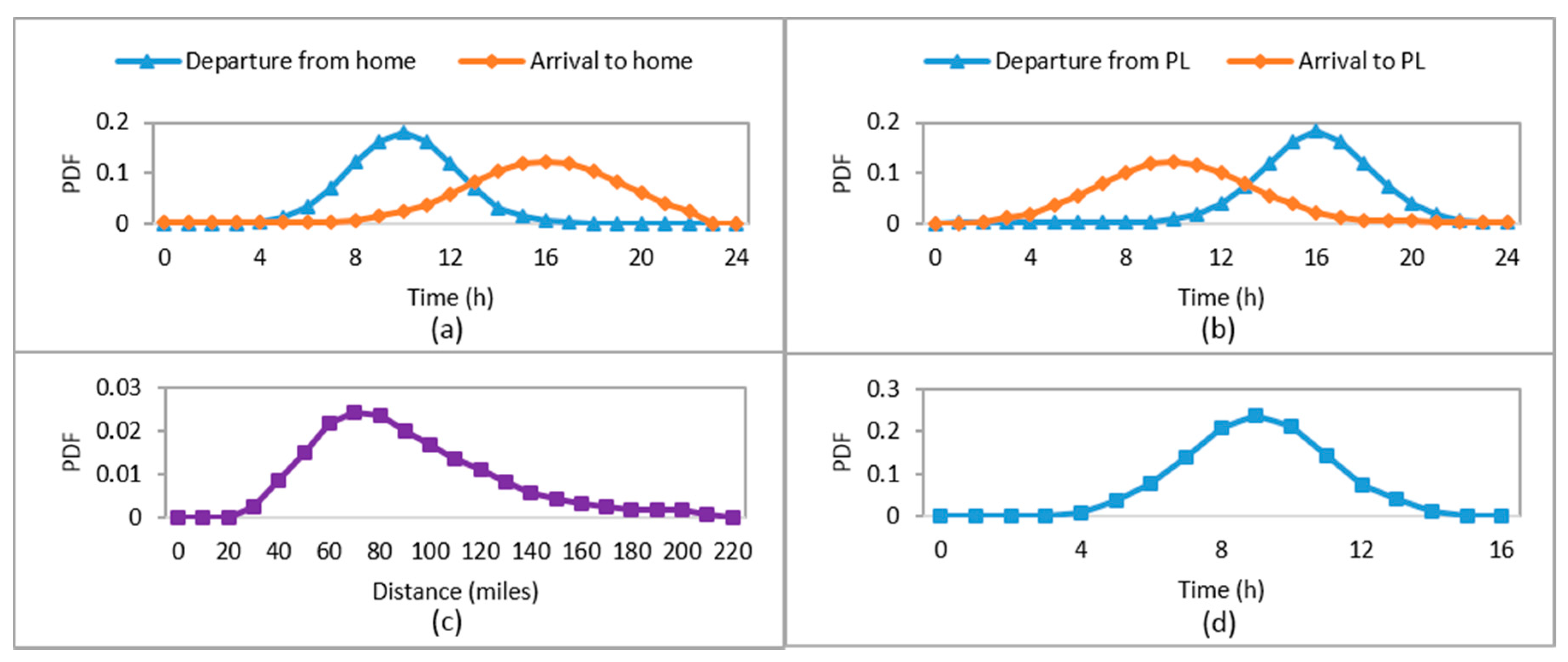
Arrival and departure PDF: The arrival time (from home to PL) and departure time (from PL to home) of EVs are considered to follow a normal distribution function as given in Equation (1) and shown in Figure 3a, and Figure 3b, respectively [32]:

$$F\left(t\right)=\frac{1}{\sqrt[\sigma ]{2\pi }}{e}^{\raisebox{1ex}{$-{\left(t-\mu \right)}^2$}\!\left/ \!\raisebox{-1ex}{$2{\sigma }^2$}\right. , 0<t<24}$$

(1)

where the mean for arrival and departure to/from home and PL are ${\mu }_{arr}^{home}=17.01$, ${\mu }_{dep}^{home}=9.97$, ${\mu }_{arr}^{PL} =10$ and ${\mu }_{dep}^{PL}=16$, respectively. Similarly, the standard deviation for arrival and departure to/from home and PL are ${\sigma }_{arr}^{home}={\sigma }_{arr}^{PL}=3.2$ and ${\sigma }_{dep}^{home}={\sigma }_{dep}^{PL}=2.2$, respectively. The mean and standard deviation values are obtained from the NHTS-2009 data based on [32].

(2)

Traveled distance PDF: A normal distribution with ${\mu }_{dis}^{tra}=3.744$ and ${\sigma }_{dis}^{tra}=0.396$ is considered for traveled distance in [33]. However, for sizable battery capacity with longer all-electric range (AER) [34], this work considers a normal distribution with ${\mu }_{dis}^{tra}=7.488$ and ${\sigma }_{dis}^{tra}=0.792$ to model the traveled distance as shown in Figure 3c.

(3)

Parking duration PDF: A normal distribution function with ${\mu }_{EV}^{PD} = 8.99$ and ${\sigma }_{EV}^{PD} = 1.92$ is considered to model the parking duration of EVs as shown in Figure 3d. The values for mean and standard deviation are given in Ref. [35] provide a reasonable parking duration; therefore, the same values are adopted in this work.

3.1.2. First Stage Fuzzy Logic Inference System

The first stage fuzzy logic inference system is modelled using three different types of linear membership functions. The readers are encouraged to refer to Ref. [19] for the definition and the detail of parameters required to implement the membership functions. The detail of inputs and output parameters for implementing the first stage FIS is given as follows.

Fuzzification of Input Parameters:

The current and required SoCs of an EV are the functions of traveled distance and next traveling trip distance, respectively. The investigation of NHTS 2009 data portrays that the daily traveled distance can be computed by correlating the two independent PDFs of arrival time and departure time events. The first stage FIS is used to correlate the arrival and departure sequence for the traveled distance of each EV. The relevant input and output parameters are the departure time from home, arrival time to PL and the traveled distance (mileage). The PDFs of departure time from home and arrival time to PL are modeled based on mean and standard deviation obtained from the real-time data of the NHTS 2009 report. The real-time data is normalized into time slots such that time slot number 1 represents 12:00 a.m., time slot number 2 represents 12:15 a.m. and so on. The set of crisp inputs needs to be fuzzified for representing it through the degree of membership functions and thus requires the definition of linguistic variables along with their units and ranges. In this work, five membership functions are selected for each of the two input variables. The first input is the departure time from home, which is measured in time slots and its range is from 5:00 a.m. to 3:00 p.m. (Figure 3a) which corresponds to the range of 21–61 in normalized time slots. The second input is the arrival time to PL, which is measured in time slots and its real-time values are from 7:00 a.m. to 5:00 p.m. (Figure 3b) which corresponds to the range of 29–69 in time slots.

The linguistic terms of the membership functions for the first input (i.e., departure time from home) are Very Early Departure from Home (VEDH), Early Departure from Home (EDH), Normal Departure from Home (NDH), Late Departure from Home (LDH) and Very Late Departure from Home (VLDH). The VEDH and VLDH are developed as left and right open shoulder membership functions.

The terms EDH, NDH and LDH are developed as triangular membership functions. The fuzzy sets VEDH and EDH contain the set of EVs having membership functions in ranges of 21 ≤ ${\mu }_{n_{EV}}$ (${\mathrm{H}}_{\mathrm{t}}^{\mathrm{dep}}$) ≤ 33 time slots and 25 ≤ ${\mu }_{n_{EV}}$ (${\mathrm{H}}_{\mathrm{t}}^{\mathrm{dep}}$) ≤ 41 time slots, respectively, where $n_{EV}$ is the number of Evs in the set. The range of time slots 33 ≤ ${\mu }_{n_{EV}}$ (${\mathrm{H}}_{\mathrm{t}}^{\mathrm{dep}}$) ≤ 49, represents the number of EV in the NDH set. Finally, the time slots ranges 41 ≤ ${\mu }_{n_{EV}}$(${\mathrm{H}}_{\mathrm{t}}^{\mathrm{dep}}$) ≤ 57 and 49 ≤ ${\mu }_{n_{EV}}$ (${\mathrm{H}}_{\mathrm{t}}^{\mathrm{dep}}$) ≤ 61, represents the number of Evs in the sets LDH and VLDH, respectively. Similarly, the membership functions of the second input (i.e., arrival time to PL) are also defined with five different linguistic terms: Very Early Arrival to Parking (VEAP), Early Arrival to PL (EAPL), Normal Arrival to PL (NAPL), Late Arrival to PL (LAPL), and Very Late Arrival to PL (VLAP).

These linguistic terms are implemented with two left-right open shoulders and three triangular membership functions. The time slots ranges 29 ≤ ${\mu }_{n_{EV}}$(${\mathrm{PL}}_{\mathrm{t}}^{\mathrm{arr}})$≤ 41 and 33 ≤ ${\mu }_{n_{EV}}$(${\mathrm{PL}}_{\mathrm{t}}^{\mathrm{arr}})$≤ 49, denotes the number of EVs in the fuzzy sets VEAPL and EAPL, respectively. The time slots range 41 ≤ ${\mu }_{n_{EV}}$(${\mathrm{PL}}_{\mathrm{t}}^{\mathrm{arr}})$ ≤ 57 holds the number of EVs in set NAPL. The ranges 49 ≤ ${\mu }_{n_{EV}}$(${\mathrm{PL}}_{\mathrm{t}}^{\mathrm{arr}})$ ≤ 65 and 57 ≤ ${\mu }_{n_{EV}}$(${\mathrm{PL}}_{\mathrm{t}}^{\mathrm{arr}})$ ≤ 69 contain the number of EVs in sets LAPL and VLAPL, respectively. The membership functions of departure time from home and arrival time to the PL are depicted in Figure 4a,b, respectively.

Fuzzy Inference System for Traveled Distance:

The fuzzy inference mechanism is basically a function of the degree of membership functions of the input and output variables and the set of expert’s rules. The inferred knowledge is the set of the fuzzy variable representing a fuzzified output. Therefore, the definition of the output variable and the fuzzification are required. In this work, the distance travelled $M^{tra}$ (mileage traveled) represents the fuzzy output variable which is modeled based on the PDF of traveled distance, discussed in Figure 3c. The robustness of the proposed TSFLIA depends upon the number of membership functions. Therefore, an adaptive experimental method of testing different numbers of membership functions was applied and the results were tested. In sequel, a total of five membership functions is selected to fuzzify the output $M^{tra}$. The variable $M^{tra}$ is fuzzified with linguistic terms Very Short Mileage Traveled (VSMT), Short Mileage Traveled (SMT), Normal Mileage Traveled (NMT), Long Mileage Traveled (LMT) and Very Long Mileage Traveled (VLMT). The VSMT and VLMT are modeled as left-open shoulder and right-open shoulder membership functions, respectively. The triangular membership functions are used to implement the terms SMT, NMT, and LMT. The traveled mileage in the range 0 < ${\mu }_{n_{EV}}$($M^{tra})$ ≤ 60 represents the number of EVs in the sets VSMT. The number of EVs with $M^{tra}$ in the range 20 ≤ ${\mu }_{n_{EV}}$($M^{tra})$ ≤ 100 is covered in the term SMT. The term NMT contains the number of EVs with $M^{tra}$ in the range of 60 ≤ ${\mu }_{n_{EV}}$($M^{tra})$ ≤ 140. Similarly, the sets LMT and VLMT contain the number of EVs with $M^{tra}$ in the ranges of 100 ≤ ${\mu }_{n_{EV}}$($M^{tra})$ ≤ 180 and 140 ≤ ${\mu }_{n_{EV}}$($M^{tra})$≤ 220, respectively. The parameters detail and membership functions of $M^{tra}$ are visualized in Figure 4c. The second step of the fuzzy inference process is to couple the fuzzy rules and the degree of membership functions. The fuzzy rules are the set of processes that map the inputs to the output using the logical IF-THEN statements [36]. The rules are designed according to the expert knowledge for the problem domain and can vary according to the different types of applications [37]. A set of fuzzy rules for the first-stage of FIS is given in

Table 1. Set of fuzzy rules of first stage FIS for computing the traveled distance.

${\mathit{M}}^{\mathit{t}\mathit{r}\mathit{a}}$		$\mathit{P}{\mathit{L}}_{\mathit{t}}^{\mathit{a}\mathit{r}\mathit{r}}$
		VEAPL	EAPL	NAPL	LAPL	VLAPL
${\mathit{H}}_{\mathit{t}}^{\mathit{d}\mathit{e}\mathit{p}}$	VEDH	VSMT	SMT	NMT	LMT	VLMT
	EDH	VSMT	SMT	SMT	NMT	LMT
	NDH	VSMT	VSMT	SMT	NMT	NMT
	LDH	VLMT	VSMT	VSMT	SMT	SMT
	VLDH	VLMT	VLMT	VSMT	VSMT	VSMT

.

Defuzzification of Traveled Distance:

The defuzzification is a process that converts the fuzzified output of FIS into crisp value. There are different standards of defuzzification methods such as the Center of Gravity (COG), Middle of Maxima (MOM), First of Maxima (FOM) and Last of Maxima (LOM) and Random Choice of Maxima (RCOM) for computing the most certain crisp value. Following our previous work, this work models the FIS using the COG method for correlating the two input variables to compute the traveled distance [19,20].

3.1.3. Problem Formulation and Objective Function

Most of the EVs are fully charged when they arrived home from work and consume energy during the day [38,39]. Therefore, SoC and the SoC^req of an EV are the functions of the traveled distance, next trip distance, all-electric range (AER) and the battery capacity and can be computed according to Equations (2) and (3) [40]:

$$So{C}_{E{V}_i}\left(t\right)= \{\begin{array}{cc}\left[1-\left(\raisebox{1ex}{$M_{E{V}_i}^{tra}$}\!\left/ \!\raisebox{-1ex}{${\mathrm{AER}}_{E{V}_i}$}\right.\right)\right]& \mathrm{if}0< M_{E{V}_i}^{tra} < \left(0.8\times {\mathrm{AER}}_{E{V}_i} \right)\hfill \\ 0.2& \mathrm{if}{M}_{E{V}_i}^{tra} \ge \left(0.8\times {\mathrm{AER}}_{E{V}_i} \right)\hfill \end{array}$$

(2)

$$So{C}_{E{V}_i}^{req}\left(t\right)= \{\begin{array}{cc}\left[\left(\raisebox{1ex}{$M_{E{V}_i}^{NTD}$}\!\left/ \!\raisebox{-1ex}{${\mathrm{AER}}_{E{V}_i}$}\right.\right)+0.2\right]& \mathrm{if}0< M_{E{V}_i}^{NTD} < \left(0.8\times {\mathrm{AER}}_{E{V}_i} \right)\hfill \\ 1& \mathrm{if} M_{E{V}_i}^{NTD} \ge \left(0.8\times {\mathrm{AER}}_{E{V}_i} \right)\hfill \end{array}$$

(3)

where ${\mathrm{AER}}_{E{V}_i}$ is the maximum distance that an ith battery electric vehicle (BEV) or Plug-in Hybrid Electric Vehicle (PHEV) can travel by using only electric energy without the use of the internal combustion engine [41]. The variables $M_{E{V}_i}^{tra}$ and $M_{E{V}_i}^{NTD}$ are the travelled and next trip distances in miles of the ith EV. To extend the battery life, a minimum margin value of SoC is considered to be 20% of the battery capacity. It is assumed the EV owners with stored energy higher than the required energy for the next trip distance are willing to sell their excess energy. Therefore, the PL control center determines the G2V and V2G operation for the EVs depending on their initial and required SoCs. Based on the difference of the initial and required SoCs, three cases can be considered to categorize the EVs for G2V, V2G and Idle operations [40].

• G2V operation: The EVs are considered to perform the G2V if their required SoCs are greater than their corresponding initial SoCs.
• V2G operation: The EVs with required SoCs less than their initial SoCs are scheduled to participate in V2G operation.
• Idle (no-participation): The EVs are considered to remain idle if their required SoCs are equivalent to their initial SoCs.

The amount of charging energy until the SoC^req and the full battery capacity in G2V operation can be computed according to Equation (4) while the amount of discharging energy in V2G operation can be computed according to Equation (5). The amount of charging and discharging of an EV is 0 (i.e., idle/no participation in G2V and V2G) if it’s current and required SoCs are equivalent, as given in Equation (6):

$$E_{E{V}_i}^{G2V}\left(t\right) =\{\begin{array}{c}B{C}_{E{V}_i} - \left({\mathrm{SoC}}_{{\mathrm{EV}}_i}\left(t\right)\times B{C}_{E{V}_i}\right),\mathrm{if} So{C}_{E{V}_i}^{req}\left(t\right) \ge B{C}_{E{V}_i}\\ \left(So{C}_{E{V}_i}^{req}\left(t\right)-{\mathrm{SoC}}_{{\mathrm{EV}}_i}\left(t\right)\right)\times B{C}_{E{V}_i},\mathrm{if} {\mathrm{SoC}}_{{\mathrm{EV}}_i}\left(t\right)< So{C}_{E{V}_i}^{req}\left(t\right) < B{C}_{E{V}_i}\end{array}$$

(4)

$$E_{E{V}_i}^{V2G}\left(t\right) =- \left({\mathrm{SoC}}_{{\mathrm{EV}}_i}\left(t\right)- So{C}_{E{V}_i}^{req}\left(t\right)\right)\times B{C}_{E{V}_i},\mathrm{if} So{C}_{E{V}_i}\left(t\right)> So{C}_{E{V}_i}^{req}\left(t\right)$$

(5)

$$E_{E{V}_i}^{V2G}\left(t\right)=0,\mathrm{if} So{C}_{E{V}_i}\left(t\right)= So{C}_{E{V}_i}^{req}\left(t\right)$$

(6)

where $E_{E{V}_i}^{G2V}$, $E_{E{V}_i}^{V2G}$, and $B{C}_{E{V}_i}$ are the charging energy, discharging energy and battery capacity of the ith EV, respectively. The total amount of required energy for the PL at each time instance t can be computed by summing up the charging and discharging energies ($E_{total}^{PL}$) of the total number of participating EVs in G2V and V2G operations, as given by Equation (7). The aggregation of baseload ($BL$) and the PL load represents the total power consumption/load ($TL)$ of any node and can be computed according to Equation (8):

$$E_{total}^{PL}\left(t\right) =\left[{\displaystyle \sum }_{i=1}^{N_{EV}}\left(E_{E{V}_i}^{G2V}- E_{E{V}_i}^{V2G}\right)\right]\left(t\right)$$

(7)

$$TL\left(t\right)=BL\left(t\right)+E_{total}^{PL}\left(t\right)$$

(8)

The baseload represents the power consumption of the customers (households, buildings, etc.) connected to a certain bus without considering the PL load. Each of the connection points (i.e., a transformer) has a defined capacity; therefore, in each scheduling period the total imported power should be maintained within the permissible limit. Since the baseload is the fundamental requirement of customers and is considered to be an uncontrolled load while the PL load is flexible and needs to be managed. The grid operators define certain boundary lines for the smooth operation of the power grid that must not be violated [42]. In this paper, these boundaries are considered to be Upper Reference Power Limit (URPL) and Lower Reference Power Limit (LRPL) for G2V and V2G operations, respectively, and given by Equations (9) and (10). The available power (AP) from the grid at any time t can thus be a function of the URPL and the baseload and can be computed as expressed by Equation (11). Similarly, the updated available power (UAP) is a function of G2V, V2G, and AP and at any time t can be computed according to Equation (12):

$$URPL{\left(t\right)}_{ }= \left(Tran{s}_{cap}- [\frac{1}{T}{\displaystyle \sum }_{t=1}^{T}BL\left(t\right)\times \omega \right)$$

(9)

$$LRPL{\left(t\right)}_{ }= B{L}_{offPeak load}\left(t\right)-[\frac{1}{T}{\displaystyle \sum }_{t=1}^{T}BL\left(t\right)\times \omega$$

(10)

$$AP\left(t\right)=URPL\left(t\right)- BL\left(t\right)$$

(11)

$$UAP\left(t\right)= \{\begin{array}{c}AP\left(t\right)- \left[{\displaystyle \sum _{i=1}^{N_{EV}}}{\left(E_{EV}^{G2V}\right)}_i\right]\left(t\right) \mathrm{if} \mathrm{charging}\\ AP\left(t\right)+\left[{\displaystyle \sum _{i=1}^{N_{EV}}}{\left(E_{EV}^{V2G}\right)}_i \right]\left(t\right) \mathrm{if} \mathrm{discharging}\end{array}$$

(12)

where $Tran{s}_{cap}$, $B{L}_{offPeak load}$, $T$ are the transformer capacity, off-peak of baseload, and total number of time slots, respectively. The term $\omega$ is a stability factor defined by the network system operators. The grid operators have to consider the correlation of the PL charging and discharging, total energy and the UAP while allocating power to the distribution transformer connected to the bus. The correlation of total PL energy (Equation (7)) and the updated available power (Equation (12)) can be defined in two cases [17]:

Case 1: The amount of total energy of PL at any time t is less than or equivalent to the updated available power. Since available power is enough to support the charging requirements of EVs; therefore, in this case, there is no need to control the charging activities of EVs. The expression of Case 1 is given by Equation (13):

$$E_{total}^{PL}\left(t\right)\le {}_{ }UAP\left(t\right)$$

(13)

Case 2: The energy demand of PL at any time t is higher than the updated available power, as given by the expression in Equation (14). In such a situation, the PL operators need to reduce the total energy demand by restricting the charging operations of certain EVs. A management algorithm is required to select the most appropriate EVs for charging operations:

$$E_{total}^{PL}\left(t\right)>{}_{ }UAP\left(t\right)$$

(14)

The TSFLIA aims to intelligently control the charging demand of EVs within the power grid URPL by allowing the most needed EVs to charge until their required SoC while shifting the charging operations of others into latter time slots. To limit the energy demand of PL during the time slots where Case 2 is applicable, we defined the objective function of minimizing the PL load with the contribution of preference (PF) variable for each of the ith EVs as expressed by Equation (15):

$$\underset{ }{\min }\left(E_{total}^{PL}\right)={{\displaystyle \sum }}_{t=1}^{P^T}C\left[{{\displaystyle \sum }}_{i=1}^{N_{EV}}\left\{\left(B{C}_{E{V}_i}\times So{C}_{E{V}_i}\right)\pm D_{E{V}_i}ɳP_{CD}\right\}\right]\left(t\right)$$

(15)

where $P^T$ is the total operating hours of the parking lot, $C$ is a binary variable representing the presence and absence of EVs with 1 and 0 at any time t, $ɳ$ is the charging and discharge efficiency, $P_{CD}$ is the charging and discharging power. The decision variable $D_{E{V}_i}$ is a binary variable and it depends on the type of EV participation, the value of PF variable, the accumulated load, URPL, and LRPL and at any time t its value can be computed by Equation (16):

$$\{\begin{array}{c}{D}_{E{V}_i}\left(t\right)=1, \mathrm{if} PF\left(t\right) \mathrm{is} \mathrm{highest} LRPL\left(t\right)<\mathrm{Total} \mathrm{load}\left(t\right) \le URPL\left(t\right)\\ D_{E{V}_i}\left(t\right)=0 , \mathrm{Otherwise}\end{array}$$

(16)

The value of the PF variable for each EV is computed by the second stage of the TSFLIA and is discussed in the subsequent section. Each of the ith EV has a stay time in parking (i.e., parking duration) with a subset of charging and discharging operation period of time. Therefore, depending on the participation of EVs in G2V and V2G, the charging and discharging period of time for each of the ith EV can be defined by Equation (17). The optimization function defined in Equation (15) has to satisfy several technical and nontechnical constraints:

$${\mathcal{T}}_{E{V}_i}^{CD}= \{\begin{array}{cc}\left(\frac{B{C}_{E{V}_i}-\left(So{C}_{E{V}_i}\ast B{C}_{E{V}_i}\right)}{P_C}\right)& \mathrm{if}\mathrm{charge}\mathrm{until}\mathrm{full}BC\hfill \\ \left(\frac{\left(So{C}_{E{V}_i}^{req}-{\mathrm{SoC}}_{{\mathrm{EV}}_i}\right) \ast B{C}_{E{V}_i}}{P_C}\right)& \mathrm{if}\mathrm{charge}\mathrm{until}So{C}^{req}\hfill \\ \left(\frac{\left(So{C}_{E{V}_i}-So{C}_{E{V}_i}^{req}\right) \ast B{C}_{E{V}_i}}{P_D}\right)& \mathrm{if}\mathrm{discharge}\mathrm{until}So{C}^{req}\hfill \end{array}$$

(17)

Parking Lot Timing Constraints: The PL has a defined starting time $t_{st}^P$ and ending time $P^T$. The arrival time and departure time of the ith EV should follow the starting and ending time of the PL as expressed by Equations (18) and (19), respectively. Also, the charging and discharging duration ${\mathcal{T}}_{E{V}_i}^{CD}$ of t the ith EV should be within its arrival to PL (${\mathrm{PL}}_{E{V}_i}^{\mathrm{arr}})$ and departure from PL (${\mathrm{PL}}_{E{V}_i}^{\mathrm{dep}})$ as expressed by Equation (20).

$$t_{st}^P\le {\mathrm{PL}}_{E{V}_i}^{\mathrm{arr}}$$

(18)

$${\mathrm{PL}}_{E{V}_i}^{\mathrm{dep}}\le P^T$$

(19)

$${\mathrm{PL}}_{E{V}_i}^{\mathrm{arr}}< {\mathcal{T}}_{E{V}_i}^{CD} \le P{L}_{E{V}_i}^{dep}$$

(20)

Battery Efficiency Constraints: The battery efficiency is an important factor which needs to be maintained during the charging and discharging operations. Each battery has a standard minimum dept of discharge (DoD) such as 20% of battery capacity, maximum $So{C}_{E{V}_i}^{max}$, and the maximum number of battery charging cycles $B_{E{V}_i}^{\max \_cyc}$ [43]. These standard limits should be satisfied at any time t during the charging and discharging operations of EVs and can be expressed by Equation (21) and Equation (22). Also, the charging and discharging power affect the battery life, therefore; at any time t, the discharging power ($P_D)$ and charging power ($P_C$) power should follow the minimum ($P_{min}^{DS})$ and maximum ($P_{max}^{CH}$) allowable power limits as expressed by Equations (23) and (24):

$$Do{D}_{E{V}_i}\le So{C}_{E{V}_i}\left(t\right)\le So{C}_{E{V}_i}^{max}$$

(21)

$${\mathrm{B}}_{E{V}_i}^{cyc}\le B_{E{V}_i}^{\max \_cyc}$$

(22)

$$P_C^{E{V}_i}\left(t\right)\le P_{max}^{CH}$$

(23)

$$-P_{min}^{DS}\le P_D^{E{V}_i}\left(t\right)$$

(24)

Total Load Constraints: The total load (i.e., the baseload and the PL) at any time t should follow the upper and lower reference power limits to maintain a smooth operation of the smart grid as expressed by Equation (25):

$$LRPL\left(t\right)\le TL\left(t\right)\le URPL\left(t\right)$$

(25)

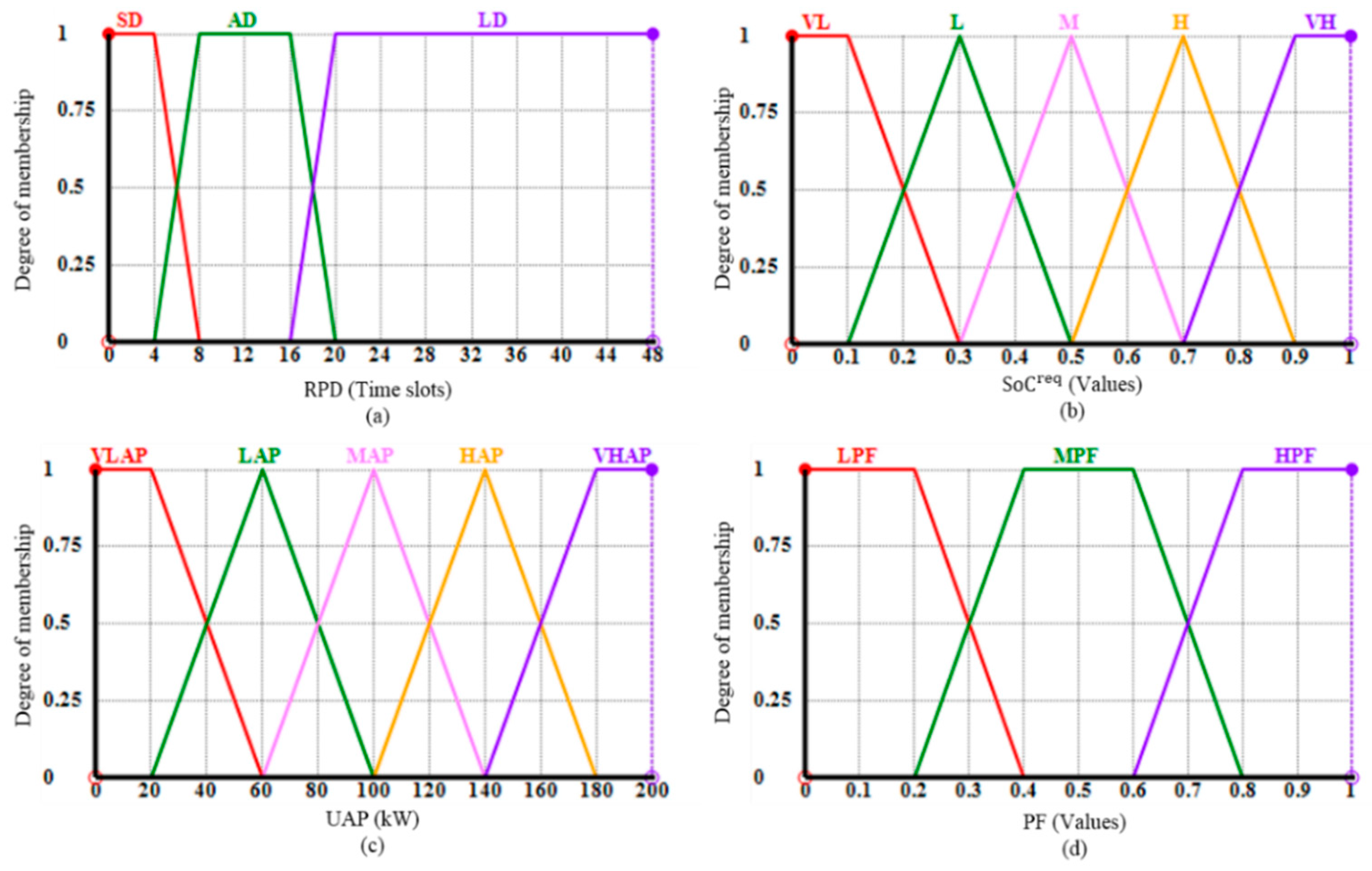
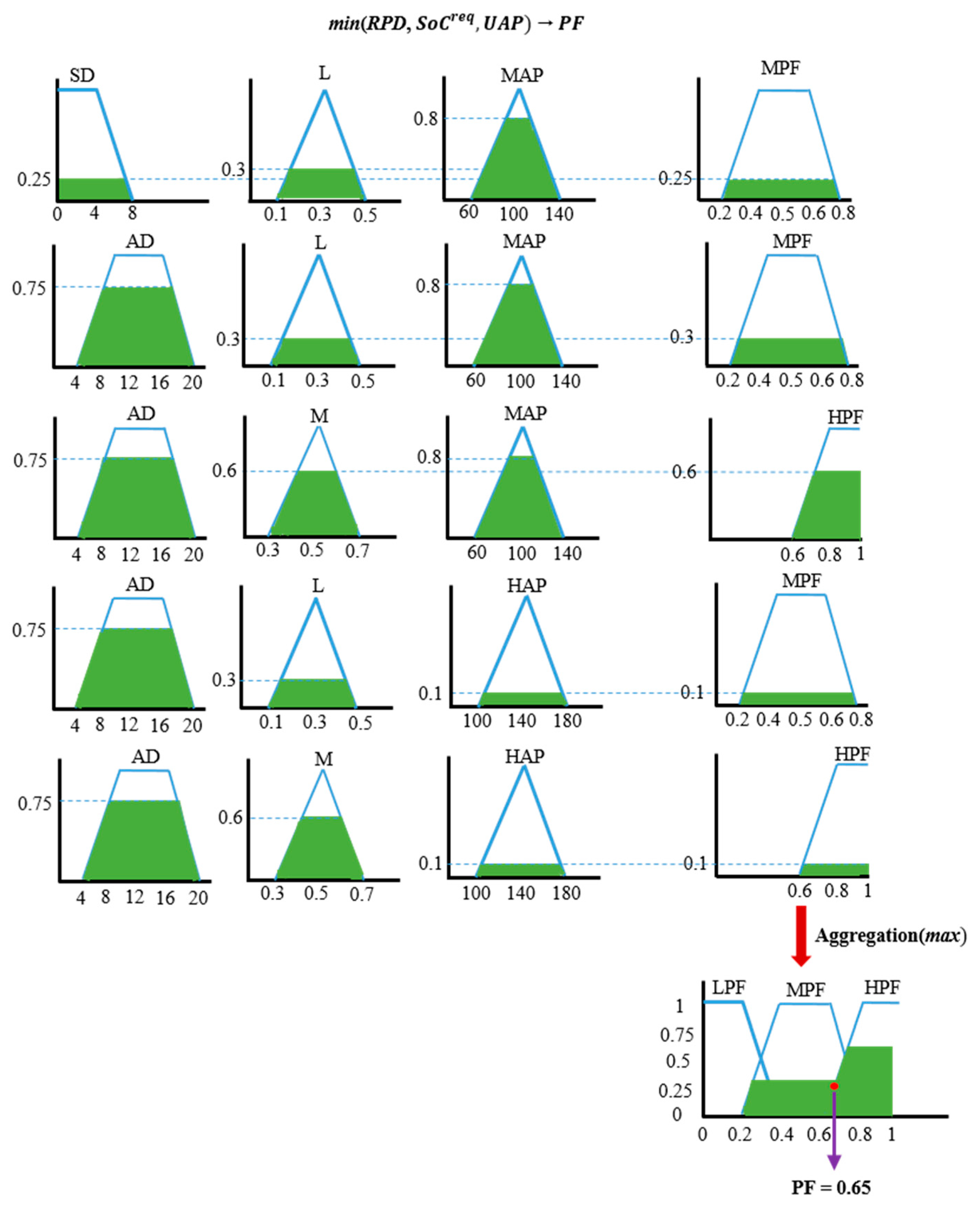
3.1.4. Second Stage Fuzzy Logic Inference System

The objective function defined in Equation (15) optimizes the energy consumption of PL using the decision variable D which is dependent on the value of the PF variable for each of the ith EV. The computation of the PF variable involves several temporal varying factors with uncertainties and is a complicated task. This work estimates an adequate value of PF through the credibility of second stage FIS, which correlates the temporal based varying uncertain parameters from the power grid and EV domains. The most admissible parameters that can influence the preference value for each of the EVs are the UAP, SoC^req, and the owner’s choice of RPD. Therefore, these parameters are considered as the input variables to the second stage of FIS. Each of the inputs is normalized and linearized in their corresponding minimum and maximum ranges and fuzzified to be represented through membership functions.

The PDF of parking duration in Figure 3d is considered to model the first input i.e., RPD. The 12 h from 4–16 h are normalized from short duration to the long duration and are linearly structured between 0 to 48 time slots. The RPD is represented through three linguistic terms: Short Duration (SD), Average Duration (AD), and Long Duration (LD) [44]. The second input is the SoC^req which is normalized from very low to very high and is represented in 0–1. The SoC^req is modeled with five linguistic terms including Very Low (VL), Low (L), Medium (M), High (H) and Very High (VH) respectively. Similarly, the UAP is normalized from low available power to high available power and is linearly structured in the range 0–200 [20]. The associated linguistic terms are Very Low Available Power (VLAP), Low Available Power (LAP), Medium Available Power (MAP), High Available Power (HAP) and Very High Available Power (VHAP). The output variable of the second stage is fuzzified with three membership functions and is linearly represented in the range of 0–1. The linguistic term for each of the output membership functions is Low Preference (LPF), Medium Preference (MPF) and High Preference (HPF). The membership functions of the inputs and output variables are graphically depicted from Figure 5a–d, respectively.

The number of inference rules depends upon the number of input variables and their membership functions [45]. There are three input variables where the first input has three membership functions and each of the other two inputs has five membership functions. To infer the knowledge for the PF variable, a total of 3 × 5 × 5 = 75 inference rules are defined in

Table 2. Set of fuzzy rules of second stage FIS when RPD is SD.

$\mathit{P}\mathit{F}$		UAP
		VLAP	LAP	MAP	HAP	VHAP
$So{C}^{req}$	VL	LPF	LPF	LPF	LPF	MPF
	L	LPF	LPF	MPF	MPF	MPF
	M	LPF	MPF	MPF	MPF	HPF
	H	MPF	APF	HPF	HPF	HPF
	VH	HPF	HPF	HPF	HPF	HPF

,

Table 3. Set of fuzzy rules of second stage FIS when RPD is AD.

$\mathit{P}\mathit{F}$		UAP
		VLAP	LAP	MAP	HAP	VHAP
$So{C}^{req}$	VL	LPF	LPF	LPF	MPF	MPF
	L	LPF	LPF	MPF	MPF	MPF
	M	LPF	LPF	HPF	HPF	HPF
	H	MPF	HPF	HPF	HPF	HPF
	VH	MPF	HPF	HPF	HPF	HPF

and

Table 4. Set of fuzzy rules of second stage FIS when RPD is LD.

$\mathit{P}\mathit{F}$		UAP
		VLAP	LAP	MAP	HAP	VHAP
$So{C}^{req}$	VL	LPF	LPF	LPF	LPF	MPF
	L	LPF	LPF	LPF	MPF	MPF
	M	LPF	LPF	MPF	MPF	MPF
	H	LPF	LPF	HPF	HPF	HPF
	VH	MPF	HPF	HPF	HPF	HPF

. The fuzzified output of the inference system is obtained through the Mamdani min-max aggregation method. The crisp value of the PF variable is obtained using the COG defuzzification method. The procedure of the Mamdani min-max aggregation method and the defuzzification of the PF variable are illustrated in the example given below.

Let at any time t, there is an EV in the PL with a battery capacity of 60 kWh, remaining parking duration of 7-time slots, and the required SoC is 0.46 (28 kWh). Let the updated available power at the time t is 105 kW. The fuzzifier of FIS convert the crisp input variables to represent them through the membership functions such that ${\mu }_{RPD}\left\{\left(SD,0.25\right),\left(AD,0.75\right)\right\}$, ${\mu }_{{\mathrm{SoC}}^{req}}\left\{\left(L,0.3\right),\left(M,0.6\right)\right\}$, and ${\mu }_{UAP}\left\{\left(MAP,0.8\right),\left(HAP,0.1\right)\right\}$. The FIS evaluates the fuzzified input variables through the implication of fuzzy rules defined in Table 2, Table 3 and Table 4, to infer the aggregated knowledge of PF output variable. For this given input data a total of eight rules are applied. The implication of these eight different rules and their corresponding output through the min operation are illustrated as follows:

Rule # 8: IF (SD, 0.25) AND (L, 0.3) AND (MAP, 0.8) THEN (MPF, 0.25)

Rule # 9: IF (SD, 0.25) AND (L, 0.3) AND (HAP, 0.1) THEN (MPF, 0.1)

Rule # 13: IF (SD, 0.25) AND (M, 0.6) AND (MAP, 0.8) THEN (MPF, 0.25)

Rule # 14: IF (SD, 0.25) AND (M, 0.6) AND (HAP, 0.1) THEN (MPF, 0.1)

Rule # 23: IF (AD, 0.75) AND (L, 0.3) AND (MAP, 0.8) THEN (MPF, 0.3)

Rule # 24: IF (AD, 0.75) AND (L, 0.3) AND (HAP, 0.1) THEN (MPF, 0.1)

Rule # 28: IF (AD, 0.75) AND (M, 0.6) AND (MAP, 0.8) THEN (HPF, 0.6)

Rule # 29: IF (AD, 0.75) AND (M, 0.6) AND (HAP, 0.1) THEN (HPF, 0.1)

Considering the discrete case of defuzzification, the value of PF variable can be computed as given below, while considering the continues case, the implication of fuzzy rules (Table 2, Table 3 and Table 4) and the value of PF variable can be obtained as depicted in Figure 6, where the rules with similar outputs are shown only once.

$$PF=\frac{\left(0.5\times 0.25\right)+\left(0.5\times 0.25\right)+\left(0.8\times 0.1\right)+\left(0.8\times 0.1\right)+\left(0.8\times 0.1\right)+\left(0.5\times 0.3\right)+\left(0.8\times 0.6\right)+\left(0.5\times 0.1\right)}{0.25+0.25+0.1+0.1+0.3+0.6+0.1+0.1}=0.65$$

The aggregated charge/discharge load of EVs affect the total power imported from the power grid. This impact is due to the simultaneous charging/discharging EVs and can be measured in terms of percentage by considering the URPL and the new peak-load as given by Equation (26). The EV owners QoE represent their level of satisfaction and is a basic factor to analyze the performance of the PL. The QoE of the EV owners is the SoC^req and for the ith EV, it can be computed based on the $So{C}_{E{V}_i}^{req}$ and $B{C}_{E{V}_i}$ as given by Equation (27). The negative sign in Equation (27) shows the discharging of EV. The EVs with satisfied and unsatisfied QoE are represented by ${\mathcal{N}}_{\mathrm{EV}}{}_{satisfied}$ and ${\mathcal{N}}_{\mathrm{EV}}{}_{Unsatisfied}$ variables, respectively. The PL QoP is the function of EVs with satisfied/unsatisfied QoE and the total number of EVs and can as given by Equation (28):

$$Load impact {(\%)}_{bu{s}_j}= \{\begin{array}{cc}\left(\frac{pea{k_{load}}_{bu{s}_j}-URP{L}_{bu{s}_j}}{pea{k_{load}}_{bu{s}_j}}\right)\ast 100& \mathrm{If} pea{k_{load}}_{bu{s}_j}> URP{L}_{bu{s}_j}\\ 0& \mathrm{Otherwise}\end{array}$$

(26)

$$Qo{E}_{E{V}_i}=\{ \begin{array}{cc}1& \mathrm{if}\mathrm{charge}\mathrm{until} B{C}_{E{V}_i}\hfill \\ So{C}_{E{V}_i}^{req} -So{C}_{E{V}_i}& \mathrm{if}\mathrm{charge}\mathrm{until}\mathrm{required} SoC\hfill \\ -\left(So{C}_{E{V}_i}- So{C}_{E{V}_i}^{req}\right)& \mathrm{if}\mathrm{discharge}\mathrm{until}\mathrm{required} SoC\hfill \\ 0& \mathrm{if}\mathrm{no}\mathrm{charge}/\mathrm{discharge}\hfill \end{array}$$

(27)

$$QoP= \left(\frac{\left|{\mathcal{N}}_{EV}\right|-{{\displaystyle \sum }}_{i=1}^{N_{EV}}E{V}_{Unsatisfied\_QoE}\left(i\right)}{\left|{\mathcal{N}}_{EV}\right|}\right)$$

(28)

3.1.5. Pseudocode of the Proposed TSFLIA

The proposed two-stage fuzzy logic inference algorithm consists of five sub-algorithms where each sub-algorithm is based on a specific function and are given as Algorithms 1–6. The pseudocode of the main TSFLIA is provided in Algorithm 1. The system global parameters including variables and the different list of elements are initialized in step 1. The EVs arrived in the previous time slot t-1 are registered in the system and are scheduled in the current slot t. The list $n_{EV}$ is used to initially store each of the newly arrived EVs. At the current time slot t, the algorithm registered all the new arrived EVs by calling the services of Algorithm 2: Manage_new_arrival. This algorithm is invoked by passing nine different global parameters, i.e., ${\mathcal{N}}_{EV},H_{EV}^{dep},P{L}_{EV}^{arr},P{L}_{EV}^{dep},B{C}_{EV},AE{R}_{EV},RP{D}_{EV}$, $M_{EV}^{NTD}, {ℳ}_{CS}$. The information from each of the EVs such as departure time from home, arrival time to PL, departure time from PL, battery capacity, and their all-electric range are collected, saved and updated in the global variables. The algorithm then checks the status of each of the CSs by iterating through the ${ℳ}_{CS}$ list of CSs. If any CS is idle, the new EV is assigned to it and the status of the CS is updated from idle to busy. After assigning the EV to the CS, the global list ${\mathcal{N}}_{EV}$ is updated by adding the new EV to it. The parking duration is calculated according to the departure and arrival time slots of each the EVs and is stored in the list $RP{D}_{EV}$. The updated information about all the new EVs is then returned to the main Algorithm 1.

The traveled distance ($M_{EV}^{tra}$) and the next trip distance ($M_{E{V}_i}^{NTD})$ are essential factors for computing the current and required SoC. To obtain the traveled distance of an EV, the sub-algorithm 3: First_stage_FLM is triggered with arguments such as $M_{EV}^{tra},H_t^{dep},P{L}_t^{arr},So{C}_{EV},So{C}_{EV}^{req},B{C}_{EV},F_{EV},j$. The algorithm loads the set of fuzzy rules from

Table 5. IEEE 34 node test feeder- spot load.

Node #	Lumped Load (kW)	Residential Load (kW)	Number of Houses
860	60	42	15
840	27	19	7
844	405	284	102
848	60	42	15
890	450	315	113
830	45	32	11
Total	1047	733	264

and evaluates the $H_t^{dep}$ and the $P{L}_t^{arr}$ through the fuzzy inference system to approximate the value of $M_{EV}^{tra}$ for each of the newly arrived EVs. Moreover, based on the computed $M_{EV}^{tra}$ and the $M_{\mathrm{EV}}^{NTD}$ (obtained from the user in Algorithm 2) the algorithm computes the $So{C}_{EV}$ and $So{C}_{EV}^{req}$ by using Equations (2) and (3). The EVs are then categorized into G2V, V2G and/or idle operations. The EVs participating in G2V operations are assigned the flag values $f_c$ for full charging until battery capacity and $p_c$ for partially charging until required SoC. The V2G and no participation (idle) of EVs are differentiated with the flag values $d_s$ and $l_d$ respectively. Finally, it returns the updated global lists of $So{C}_{EV},So{C}_{EV}^{req}$ and $F_{EV}$ to the main algorithm. In the case, if there is no arrival of any new EV such that $n_{EV}$ = 0, the algorithm proceeds with the consequent steps and based on the number of EVs requesting for discharging operations, it computes the updated available power for the current time t according to Equation (12). The total number ($N_{EV}^{cha}$) of EVs that can be supported by the updated available power is computed in step 19. From step 20 to step 25, the Algorithm 1 iterates through each of the CSs to check their status, if there are connected EVs with remaining parking duration their G2V and V2G operations are then scheduled by triggering the Algorithm 4: Second_stage_FLM. The services of this sub-algorithm are called by passing the list of arguments such as $UAP,P{F}_{EV},RP{D}_{EV},So{C}_{EV}^{req},So{C}_{EV},N_{EV}^{cha},D_{EV},i,j,$ to it. In this sub-algorithm, the fuzzy inference mechanism evaluates the $UAP$, $RP{D}_{EV}$ and $So{C}_{EV}^{req}$ to approximate the preference value for the current EV and then resort the updated list of preferences values i.e., $P{F}_{EV}$ in descending order. Based on the total number of allowable EVs, the sorted list $P{F}_{EV}$, and the current and require SoCs the list $D_{EV}$ is updated and constraints defined by Equations (21) and (22) are validated. This updated lists $P{F}_{EV}$ and $D_{EV}$ are then returned to the main Algorithm 1.

Algorithm 1:	Two-Stage Fuzzy Logic Inference Main Algorithm

The scheduled charging and discharging operations for each of the EV is then handled through the sub-algorithm 5: Manage_charge_discharge. The services of this algorithm are called by passing eleven different arguments, i.e., $D_{EV},UAP,$ $F_{EV},So{C}_{EV},BL,TL,P_C,P_D,\eta ,i,j$. It considers the updated lists of $UAP$, $D_{EV}$ and $F_{EV}$ while performing charging (i.e., partial charging until required SoC or full charging until battery capacities), discharging (until required SoCs) and idle operations for each of the EV. The charging and discharging operations update the lists $So{C}_{EV}$ for each the EVs and effect (increase/decrease) the list $UAP$, while retaining the previous values of these parameters with the idle operation of EVs. The total load at the current time slot t is then computed and the value is updated in the global list $TL$. Finally, the updated lists of the SoCs for each of the EVs and the TL are returned to the main algorithm. Lastly, the sub-algorithm 6: Manage_departure is invoked by passing the arguments such as ${\mathcal{N}}_{EV}$,$So{C}_{EV}$,$So{C}_{EV}^{req},B{C}_{EV},Qo{E}_{sucf},Qo{E}_{unsucf},i$ to handle the departure of the EVs. It checks the $So{C}_{EV}$ against the $So{C}_{EV}^{req}$ and $B{C}_{EV}$ to measure the satisfaction of the EV owners QoE and accordingly update the variables $Qo{E}_{sucf}$ if QoE is successful and $Qo{E}_{unsucf}$ if QoE is unsuccessful for each of the departing EVs. The departure event resulting in updating the list ${\mathcal{N}}_{EV}$ (i.e., decrement the departing EV from the list). The updated list ${\mathcal{N}}_{EV}$ and the variables $Qo{E}_{sucf}$ and $Qo{E}_{unsucf}$ are returned to the main algorithm. The main algorithm updates the list of $RPD$ for the departing EV while incrementing the current time slot by 1. The algorithm repeats the whole process from step 3 to 35 until the end of the simulation time. Finally, in steps 37 and 38 the statistics such as the impact on the total load, the EV owners QoE and the PL QoP are computed according to the Equation (26), Equations (27) and (28), respectively.

Algorithm 2	Manage_new_arrivals (${\mathcal{N}}_{EV},H_{EV}^{dep},P{L}_{EV}^{arr},P{L}_{EV}^{dep},B{C}_{EV},AE{R}_{EV},RP{D}_{EV}$,$M_{EV}^{NTD},$${ℳ}_{CS}$)

Algorithm 3	First_stage_FLM ($M_{EV}^{tr},H_t^{dep},P{L}_t^{arr},So{C}_{EV},So{C}_{EV}^{req},B{C}_{EV}, F_{EV},j$)
1.	FIS.load(rules file) */ Load the fuzzy rule file from Table 1 */
2.	/* Evaluate through FIS and categorize the EVs into G2V, V2G, and idle using Equations (4)–(6) */ $M_{EV}^{tr}\left[j\right]\leftarrow \mathrm{FIS}.\mathrm{Evaluate}\left(H_t^{dep}\left[j\right],P{L}_t^{arr}\left[j\right]\right)$
3.	${\mathrm{SoC}}_{EV}\left[j\right]$$\leftarrow \left[\left[1-\left(\raisebox{1ex}{$M_{EV}^{tra}\left[j\right]$}\!\left/ \!\raisebox{-1ex}{${\mathrm{AER}}_{EV}\left[j\right]$}\right.\right)\right] \ast B{C}_{EV}\left[j\right]\right]$or$\left(0.2 \ast B{C}_{EV}[j\right)$
4.	$So{C}_{EV}^{req}\left[j\right]$$\leftarrow$$\left[\left[\left[\left(\raisebox{1ex}{$M_{EV}^{NTD}\left[j\right]$}\!\left/ \!\raisebox{-1ex}{${\mathrm{AER}}_{EV}\left[j\right]$}\right.\right)\right]+0.2\right] \ast B{C}_{EV}\left[j\right]\right]$or$B{C}_{EV}\left[j\right]$
5.	If ($So{C}_{EV}^{req}\left[j\right]\ge$ $B{C}_{EV}$[j])
6.	|$F_{EV}\left[j\right]$$\leftarrow$$f_c$. /* Set flag for full charge and compute QoE according to Equation (27) */
7.	Else if ($So{C}_{EV}^{req}\left[j\right]>So{C}_{EV}\left[j\right] \&\& So{C}_{EV}^{req}\left[j\right]<$ $B{C}_{EV}$[j])
8.	|$F_{EV}\left[j\right]$$\leftarrow$$p_c$ /* Set flag for partial charge and compute QoE according to Equation (27) */
9.	Else if ($So{C}_{EV}^{req}\left[j\right]$$==So{C}_{EV}\left[j\right]$)
10.	|$F_{EV}\left[j\right]\leftarrow$$l_d$ /* Set flag for idle and compute QoE according to Equation (27) */
11.	Else if ($So{C}_{EV}\left[j\right]>So{C}_{EV}^{req}\left[j\right]$)
12.	|$F_{EV}\left[j\right]$$\leftarrow$$d_s$ /* Flag for discharge and compute QoE according to Equation (27) */
13.	End
14.	Return updated $So{C}_{EV}, So{C}_{EV}^{req},$ and $F_{EV}$

Algorithm 4	Second_stage_FLM$(UAP,P{F}_{EV},RP{D}_{EV},So{C}_{EV}^{req},So{C}_{EV},N_{EV}^{cha},D_{EV},i,j$)

Algorithm 5	Manage_charge_discharge ($D_{EV},UAP$$F_{EV},So{C}_{EV},BL,TL,P_C,P_D,\eta ,i,j$)

Algorithm 6	Manage_departure (${\mathcal{N}}_{EV}$,$So{C}_{EV}$,$So{C}_{EV}^{req},B{C}_{EV},Qo{E}_{sucf},Qo{E}_{unsucf},i$)
1.	Check the departure time constraints defined by Equation (19)
2.	If ($So{C}_{EV}\left[i\right]\ge B{C}_{EV}\left[i\right] \left|\right| So{C}_{EV}\left[i\right]\ge So{C}_{EV}^{req}\left[i\right]$)
3.	|$Qo{E}_{sucf}$$\leftarrow$$Qo{E}_{sucf}$ + 1
4.	Else if ($So{C}_{EV}\left[i\right]\le So{C}_{EV}^{req}\left[i\right]$)
5.	|$Qo{E}_{unsucf}$$\leftarrow$$Qo{E}_{unsucf}$ + 1
6.	End if
7.	${\mathcal{N}}_{EV}\left[i\right]$$\leftarrow$${\mathcal{N}}_{EV}\left[i\right]$ −1 /*Decrement list of EVs*/
8.	Return updated ${\mathcal{N}}_{EV}, Qo{E}_{sucf}$ and $Qo{E}_{unsucf}$

4. Simulation Results and Discussion

4.1. Simulation Setting and Assumption

This study adopts the IEEE 34-node bus system which is downscaled from 24.9 kV to 230 V such that this power network represents a residential distribution system [46]. The modified layout of the IEEE 34-node network is presented in Figure 7 which has six spot loads, and 27 distributed loads and the bus number 800 is connected to the power transmission source [47]. The total residential load of each node depends upon the total number of connected houses and their consumption in a day. We assume an average household consumption of about 2.78 kW [48] and a load factor of 70% for each lumped loads of IEEE 34-node system to determine the number of connected houses as given by Equation (29) [49]. The number of connected houses to each of the buses is computed for the six spot loads and 27 distributed loads and is given in the last column of Table 5 and

Table 6. IEEE 34 node test feeder- distributed load.

From Bus #	To Bus #	Lumped Load (kW)	Assumed Residential Load (kW)	Number of Houses
802	806	55	39	14
808	810	16	11	4
818	820	34	24	9
820	822	135	95	34
816	824	5	4	1
824	826	40	28	10
824	828	4	3	1
828	830	7	5	2
854	856	4	3	1
832	858	15	11	4
858	864	2	1	1
858	834	32	22	8
834	860	146	102	37
860	836	82	57	21
836	840	40	28	10
862	838	28	20	7
842	844	9	6	2
844	846	45	32	11
846	848	23	16	6
Total		722	505	182

, respectively. The candidate buses for the PL are assumed to be 808, 810, 820, 822, 826, 828, 834, 838, 844, 846, and 856. This work assumes three PLs connected to bus number 820, 834, and 844, respectively. The total residential load (i.e., baseload) profiles connected to these buses is shown in Figure 8. Most of the PLs are operating during the daytime, such that they have operation hours $P^T$ from morning 7:00 a.m. to 7:00 p.m. evening [49]. Thus, the simulation is carried out for 12 h where each hour is sampled with a 15 min resolution. The total number of time slots $T_{max}$ is thus computed as 48-time slots. The entire system is developed using Eclipse software where the jFuzzyLogic libraries are utilized to build up the two stages of FIS [50]. The EVs considered in this work are of four different types such as Nissan LEAF with 40.0 kWh battery, Tesla-S with 60.0 kWh battery, Tesla model-3 with 80.5 kWh battery, and Tesla model-X with 100.0 kWh battery, respectively [51,52,53,54]. The AER of an EV is a function of battery capacity and its energy consumption rate and can be obtained through Equation (30) [49].

$$House{s}_{bu{s}_j}=⎾\frac{Lumped\_loa{d}_{bu{s}_j}\ast load\_facto{r}_{bu{s}_j}}{Avg\_consumptio{n}_{house}}⏋$$

(29)

$$AE{R}_{E{V}_i}=\frac{B{C}_{E{V}_i}}{EC{R}_{E{V}_i}}$$

(30)

where $EC{R}_{E{V}_i}$ is the energy consumption rate of the ith EV and is measured in kWh per mile. This work considered the $ECR$ values 0.34, 0.36, 0.38, and 0.37 kWh/mile for Nissan LEAF, Tesla-S, Tesla model-3 and Tesla model-X, respectively [55]. In this way, the AERs obtained for the four types of EVs are 115 miles, 165 miles, 210 miles, and 270 miles, respectively. A total of 200 EVs is randomly distributed with different penetration levels for each type of EVs as shown in

Table 7. Random distribution of different type of EVs.

Cases	Nissan LEAF-40 kWh [51]	Tesla S-60 kWh [52]	Tesla Model-3 80.5 kWh [53]	Tesla Model X- 100 kWh [54]
1	23%	28%	18%	31%
2	26%	21%	29%	24%
3	28%	21%	25%	25%

. In this work it is assumed that each of the parking spots has a fast CS, where each of the CS has charge/discharge rate of 20 kWh [56] and the EVs owners provide the information of the next traveling distance to the PL operators. Three different scenarios are simulated for buses number 820, 834 and 844, where the PLs are connected. The departure time from home is randomly generated with a $\mu =41$ slot-number and $\sigma =$ 8 time-slots using Gaussian distribution. The arrival time and departure time to/from the PL are randomly generated with the mean values of time slot numbers 49 and 55, respectively, and a $\sigma =$12-time slots through Gaussian distribution. These random behaviors of EVs for the three PLs connected to buses number 820, 834, and 844 are depicted in Figure 9. The random arrival and departure sequence of EVs results in a different parking duration or parking occupancy, as shown in Figure 10. The lumped load of the three buses is considered for assuming the $Tran{s}_{cap}$ capacity and similarly the average load profile is considered for the value of $\mathsf{\omega }$, which is 10% of the average load profile. The charging and discharging efficiency η is considered to be about 0.90 [57].

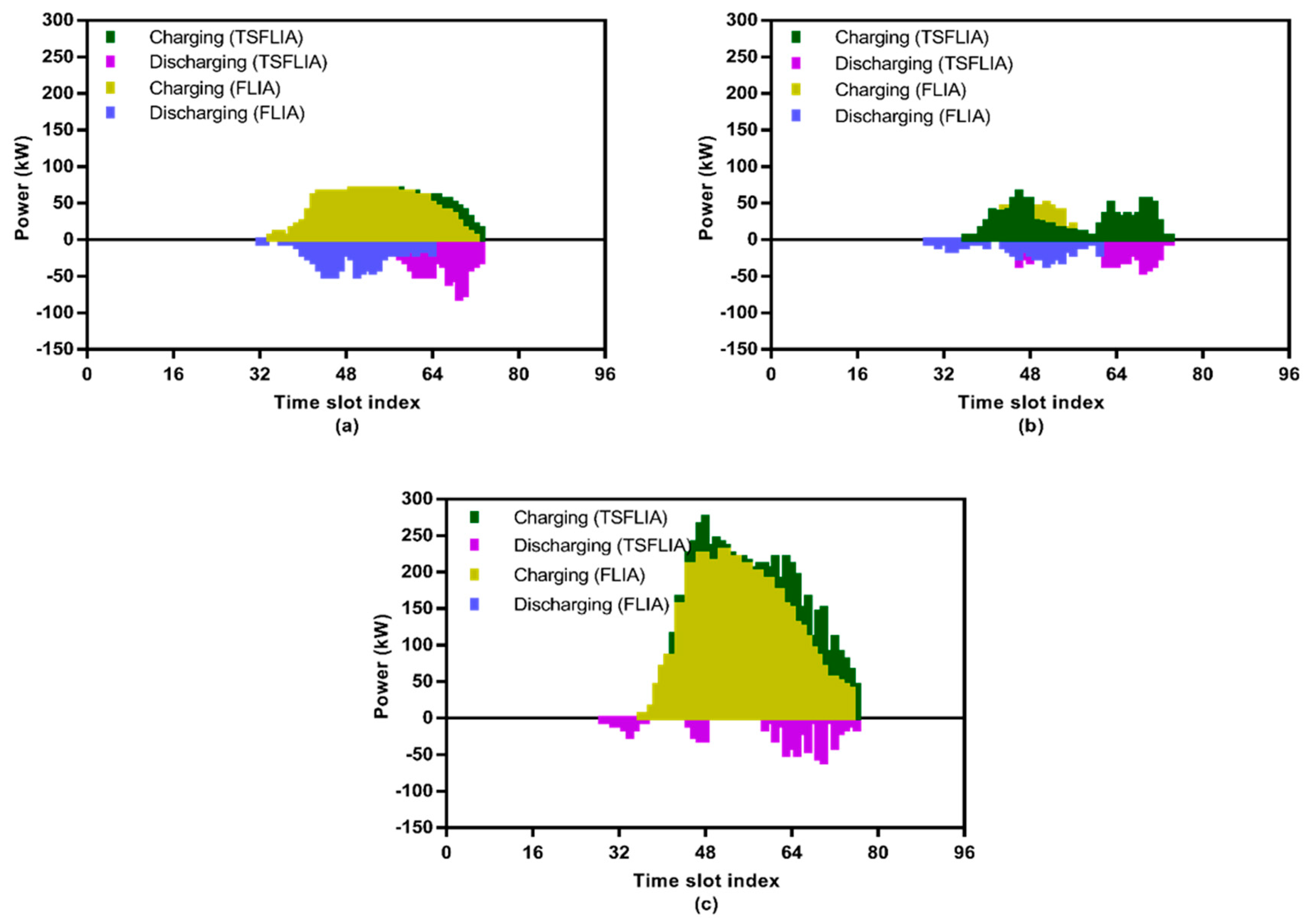
4.2. Simulation Results

To evaluate the TSFLIA scheme, the performance of the proposed TSFLIA is compared with the scheme given in [20]. The scheme given in [20] is more effective as compared to the conventional FCFS-based scheme; however, with time as the parking occupancies increases, its performance degrades in terms of the EV owner’s QoE. The reason for this performance degradation is due to the inefficient assumption made for charging and discharging of the EVs. Two types of requirements such as the power grid operation limits and the PL QoP in terms of QoE satisfaction for the EV owners are considered as the performance criteria. The power grid operation is the function of URPL and the peak-load and is measured in terms of the percentage. The EV owner’s QoE refers to the amount of charge/discharge energies of EVs required at their departure time and thus representing their level of satisfaction. The QoP is the ratio of EVs with QoE to the total number of EVs.

The results in Figure 11 show the battery capacities, the SoCs and SoC^req of EVs in the PL connected to buses number 820, 834 and 844, respectively. The SoCs at the time of arrival are computed based on their traveled distance, while the required SoCs are computed according to their next traveling distance. It can be observed that in each of the PLs, a different number of EVs are requesting for charging and discharging operations. The EVs requesting the charging operations are about 58%, 61.5% and 66.5%, while the EVs with discharging requests are about 42%, 38.5% and 33.5% in the PLs at buses number 820, 834 and 844, respectively. The charging and discharging behaviors of these PLs with respect to the two different schemes are shown in Figure 12. The FLIA schedules the EVs according to the logic α-cut and β-cut properties of fuzzy logic theory where these values were set as α = 0.8 and β = 0.3. The EVs with the value of PF variable equal to or less than β values are scheduled for charging while those with the value of PF variable equal to or greater than α are scheduled for discharging operations. The TSFLIA computes the required SoC according to the next trip traveling distance and utilizes the available power more efficiently for maximizing the EV owners QoE.

In PL 820 (Figure 12a), a consistent charging and discharging between the time slots 35 to 64 can be observed with FLIA. The TSFLIA performs the charging and discharging operations according to the required SoC and mitigates the charging load by keeping those EVs withhold which have longer stay time. Their recharging is performed in the later time slots as can be observed from time slots 62 to 77. In PL 834 (Figure 12b), the FLIA and TSFLIA perform the charging and discharging operations differently according to the scheduling mechanism of the algorithms which considers the remaining parking duration, required SoCs, and the available power, respectively. The FLIA schedule the charging and discharging for most of the EVs between time slots 45 to 64. While the TSFLIA first charge the EVs between time slots 40 to 56 where the peak charging is at time slot 48 and then perform the requested charging and discharging between time slots 63 to 75. Due to the limited power availability and discharging more number of EVs, the charging behavior with the FLIA scheme is not significant as compared to the TSFLIA scheme.

In PL 844 (Figure 12c), a limited number of EVs are scheduled for discharging with the FLIA scheme. This is because the available power is enough to accommodate the charging load of EVs. However, in this case, the TSFLIA discharge only those EVs which requested the V2G operations.

Following the charging and discharging behavior of EVs, the aggregated total load with respect to each scheme for buses number 820, 834 and 844 are shown in Figure 13. The URPL for each for each of the buses is computed according to the baseload and the transformer capacity of the buses. The URPL for bus number 820 is 128.13 kW, 146.88 kW for bus number 834, and 376.16 kW for bus number 844, as shown with red dashed lines (Figure 13). Both the FLIA and TSLFIA schemes are respecting the power grid operational limits and thus keeps the total load within the URPL. The TSFLIA charges the EVs until their required SoCs while FLIA charges the EVs until their battery capacities. Therefore, the TSFLIA is able to efficiently utilize the available power and satisfy the QoE for most of the EVs as compared to the FLIA. Each of the two schemes results in a different QoP measurement as shown in Figure 14.

For all the PLs connected to the three buses, the TSFLIA scheme achieves a higher QoP as compared to the FLIA. The QoP with FLIA and TSFLIA is 57.5% and 68.5%, respectively, (Figure 14a) for the PL connected to the bus number 820. Similarly, the QoP of the PL connected to the bus number 834 is about 27% with FLIA and 46% with TSFLIA as can be observed from Figure 14b.

The reason for this low QoP is due to the limited huge baseload which results in limited available power. A progressive performance in terms of QoP with the two schemes at PL connect to bus number 844 can be observed in Figure 14c. The reason is that there is enough available power that fulfills the QoE for more EV owners during their parking duration. The PL attached to bus number 844 has 72% with FLIA scheme, and 85% with the proposed TSFLIA scheme, as can be seen from Figure 14c. The results of PL at bus number 820 show that the QoP with TSFLIA has been improved by about 20% compared to the FLIA scheme. In the case of PLs connected to buses number 834 and 844, the results depict that the TSFLIA has a higher QoP of about 19% and 13%, respectively, compared to the FLIA scheme. This implies that when the available power is limited, the scheduling for discharging EVs results in obtaining a higher QoP.

5. Conclusions

In this paper, we proposed a two-stage fuzzy logic inference based algorithm to schedule the charging and discharging operations of EVs that maximized the quality of performance for PLs under the operational constraints of the power grid. The probability density functions of EVs arrival and departure times obtained from the NHTS data have been utilized to model the first stage fuzzy inference mechanism which calculates the amount of charging and discharging energies of EVs according to their next trip distances. Based on the energy requirements, the operations of EVs were categorized into G2V, V2G and idle. Once the EVs participations and their energy requirements were known, the services of the second stage fuzzy inference mechanism were exploited to control the operations of EVs. The proposed scheme was applied to three PLs connected to the buses number 820, 834 and 844 of the IEEE 34-node distribution system. The simulation was carried out by considering 200 EVs with different penetration levels for each of the PLs. The simulation results verified the feasibility and effectiveness of the proposed scheme against the FLIA scheme. In more detail, the TSFLIA has maximized the QoP by about 11%, 19%, and 13% compared to FLIA for the PLs connected to the buses number 820, 834, and 844, respectively.

Research limitations: There are several other aspects such as forecasting the next trip distance and robustness analysis in terms of time analysis & fairness of the proposed algorithm. In the future, the work will be extended with sophisticated scenarios for approximating an adequate next trip distance requirement using neural network models, and conducting fairness and time analysis (i.e., complexity and execution time).

Research Implications: In order to realize the role of electric vehicles as prosumers, the future parking lots are regarded as a platform that can efficiently utilize the EVs aggregated load as well as the power supply resources in grid-to-vehicle and vehicle-to-grid modes. Therefore, there is a need to study the implications of EVs parking lots by developing models for sustainable development such as social, environmental and market economics.

References

1. Nour, M.; Said, S.M.; Ali, A.; Farkas, C. Smart Charging of Electric Vehicles According to Electricity Price. In Proceedings of the Conference on Innovative Trends in Computer Engineering (ITCE), Aswan, Egypt, 8–9 February 2020; pp. 432–437. [Google Scholar]
2. Tan, K.M.; Ramachandaramurthy, V.K.; Yong, J.Y.; Padmanaban, S.; Mihet-Popa, L.; Blaabjerg, F. Minimization of load variance in power grids—Investigation on optimal vehicle-to-grid scheduling. Energies 2017, 10, 1880. [Google Scholar] [CrossRef] [Green Version]
3. Neyestani, N.; Catalão, J.P. The value of reserve for plug-in electric vehicle parking lots. In Proceedings of the 2017 IEEE Manchester PowerTech, Manchester, UK, 18–22 June 2017; pp. 1–6. [Google Scholar]
4. Neyestani, N.; Damavandi, M.Y.; Shafie-Khah, M.; Bakirtzis, A.G.; Catalão, J.P. Plug-in electric vehicles parking lot equilibria with energy and reserve markets. IEEE Trans. Power Syst. 2016, 32, 2001–2016. [Google Scholar] [CrossRef]
5. Moghaddam, Z.; Ahmad, I.; Habibi, D.; Phung, Q.V. Smart charging strategy for electric vehicle charging stations. IEEE Trans. Transp. Electrif. 2017, 4, 76–88. [Google Scholar] [CrossRef]
6. Hariri, A.O.; El Hariri, M.; Youssef, T.; Mohammed, O.A. A bilateral decision support platform for public charging of connected electric vehicles. IEEE Trans. Veh. Technol. 2018, 68, 129–140. [Google Scholar] [CrossRef]
7. An, J.; Wen, G.; Xu, W. Improved results on Fuzzy H∞ filter design for TS Fuzzy systems. Discret. Dyn. Nat. Soc. 2010, 2010, 1–21. [Google Scholar] [CrossRef] [Green Version]
8. An, J.; Li, T.; Wen, G.; Li, R. New stability conditions for uncertain TS fuzzy systems with interval time-varying delay. Int. J. Control Autom. Syst. 2012, 10, 490–497. [Google Scholar] [CrossRef]
9. Park, J.; Sim, Y.; Lee, G.; Cho, D.-H. A Fuzzy Logic Based Electric Vehicle Scheduling in Smart Charging Network. In Proceedings of the 2019 16th IEEE Annual Consumer Communications & Networking Conference (CCNC), Las Vegas, NV, USA, 11–14 January 2019; pp. 1–6. [Google Scholar]
10. Hariri, A.O.; Esfahani, M.M.; Mohammed, O. A Cognitive Price-Based Approach for Real-Time Management of En-Route Electric Vehicles. In Proceedings of the 2018 IEEE Transportation Electrification Conference and Expo (ITEC), Long Beach, CA, USA, 15 June 2018; pp. 922–927. [Google Scholar]
11. Sah, B.; Kumar, P.; Rayudu, R.; Bose, S.K.; Inala, K.P. Impact of Sampling in the Operation of Vehicle to Grid and its Mitigation. IEEE Trans. Ind. Inform. 2018, 15, 3923–3933. [Google Scholar] [CrossRef]
12. Singh, M.; Kumar, P.; Kar, I. Implementation of vehicle to grid infrastructure using fuzzy logic controller. IEEE Trans. Smart Grid 2012, 3, 565–577. [Google Scholar] [CrossRef]
13. Mehta, R.; Srinivasan, D.; Trivedi, A. Optimal Charging Scheduling of Plug-In Electric Vehicles for Maximizing Penetration within a Workplace Car Park. In Proceedings of the 2016 IEEE Congress on Evolutionary Computation (CEC), Vancouver, BC, Canada, 24–26 July 2016; pp. 3646–3653. [Google Scholar]
14. Mirzaei, M.J.; Kazemi, A.; Homaee, O. A probabilistic approach to determine optimal capacity and location of electric vehicles parking lots in distribution networks. IEEE Trans. Ind. Inform. 2015, 12, 1963–1972. [Google Scholar] [CrossRef]
15. Yao, L.; Damiran, Z.; Lim, W.H. A Fuzzy Logic Based Charging Scheme for Electric Vechicle Parking Station. In Proceedings of the 2016 IEEE 16th International Conference on Environment and Electrical Engineering (EEEIC), Florence, Italy, 7–10 June 2016; pp. 1–6. [Google Scholar]
16. Akhavan-Rezai, E.; Shaaban, M.F.; El-Saadany, E.F.; Karray, F. Online Intelligent Demand Management of Plug-In Electric Vehicles in Future Smart Parking Lots. IEEE Syst. J. 2015, 10, 483–494. [Google Scholar] [CrossRef]
17. Jiyao, A.; Tang, J.; Yu, Y. Fuzzy Multi-Objective Optimized with Efficient Energy and Time-Varying Price for EV Charging System. In Proceedings of the Proceedings on the International Conference on Artificial Intelligence (ICAI), Las Vegas, NV, USA, 12–15 July 2010; pp. 47–53. [Google Scholar]
18. Mohamed, A.; Salehi, V.; Ma, T.; Mohammed, O. Real-time energy management algorithm for plug-in hybrid electric vehicle charging parks involving sustainable energy. IEEE Trans. Sustain. Energy 2013, 5, 577–586. [Google Scholar] [CrossRef]
19. Hussain, S.; Ahmed, M.A.; Lee, K.-B.; Kim, Y.-C. Fuzzy Logic Weight Based Charging Scheme for Optimal Distribution of Charging Power among Electric Vehicles in a Parking Lot. Energies 2020, 13, 3119. [Google Scholar] [CrossRef]
20. Hussain, S.; Ahmed, M.A.; Kim, Y.-C. Efficient Power Management Algorithm Based on Fuzzy Logic Inference for Electric Vehicles Parking Lot. IEEE Access 2019, 7, 65467–65485. [Google Scholar] [CrossRef]
21. Vaidya, B.; Mouftah, H.T. Smart electric vehicle charging management for smart cities. IET Smart Cities 2020, 2, 4–13. [Google Scholar] [CrossRef]
22. Wang, G.; Zhang, Y.; Fang, Z.; Wang, S.; Zhang, F.; Zhang, D. FairCharge: A data-driven fairness-aware charging recommendation system for large-scale electric taxi fleets. Proc. ACM Interact. Mob. Wearable Ubiquitous Technol. 2020, 4, 1–25. [Google Scholar] [CrossRef] [Green Version]
23. Dubey, A.; Santoso, S. Electric vehicle charging on residential distribution systems: Impacts and mitigations. IEEE Access 2015, 3, 1871–1893. [Google Scholar] [CrossRef]
24. Kuran, M.Ş.; Viana, A.C.; Iannone, L.; Kofman, D.; Mermoud, G.; Vasseur, J.P. A smart parking lot management system for scheduling the recharging of electric vehicles. IEEE Trans. Smart Grid 2015, 6, 2942–2953. [Google Scholar] [CrossRef]
25. Hussain, S.; Muhammad, F.; Kim, Y.-C. Communication Network Architecture Based on Logical Nodes for Electric Vehicles. In Proceedings of the 2017 International Symposium on Information Technology Convergence, Shijiazhuang, China, 19–21 October 2017; pp. 321–326. [Google Scholar]
26. Nijhuis, M.; Gibescu, M.; Cobben, J. Valuation of measurement data for low voltage network expansion planning. Electr. Power Syst. Res. 2017, 151, 59–67. [Google Scholar] [CrossRef]
27. National Household Travel Survey. Available online: http://nhts.ornl.gov (accessed on 1 January 2019).
28. Tan, J.; Wang, L. Integration of plug-in hybrid electric vehicles into residential distribution grid based on two-layer intelligent optimization. IEEE Trans. Smart Grid 2014, 5, 1774–1784. [Google Scholar] [CrossRef]
29. Mu, Y.; Wu, J.; Jenkins, N.; Jia, H.; Wang, C. A spatial–temporal model for grid impact analysis of plug-in electric vehicles. Appl. Energy 2014, 114, 456–465. [Google Scholar] [CrossRef] [Green Version]
30. Rezaee, S.; Farjah, E.; Khorramdel, B. Probabilistic analysis of plug-in electric vehicles impact on electrical grid through homes and parking lots. IEEE Trans. Sustain. Energy 2013, 4, 1024–1033. [Google Scholar] [CrossRef]
31. Stephens, T. An Agent-Based Model of Energy Demand and Emissions from Plug-In Hybrid Electric Vehicle Use. Master’s Thesis, University of Michigan, Ann Arbor, MI, USA, 31 August 2010. [Google Scholar]
32. Preethi, A.A.; Nesamalar, J.J.D.; Suganya, S.; Raja, S.C. Economic Scheduling of Plug-In Hybrid Electric Vehicle Considering Various Travel Patterns. In Proceedings of the 2018 National Power Engineering Conference (NPEC), Madurai, India, 9–10 March 2018; pp. 1–7. [Google Scholar]
33. Mendoza, C.C.; Quintero, A.M.; Santamaria, F. Estimation of electric energy required by electric vehicles based on travelled distances in a residential zone. Tecciencia 2016, 11, 17–24. [Google Scholar] [CrossRef]
34. Du, J.; Li, F.; Li, J.; Wu, X.; Song, Z.; Zou, Y.; Ouyang, M. Evaluating the technological evolution of battery electric buses: China as a case. Energy 2019, 176, 309–319. [Google Scholar] [CrossRef]
35. Ma, T.; Mohammed, O.A. Optimal charging of plug-in electric vehicles for a car-park infrastructure. IEEE Trans. Ind. Appl. 2014, 50, 2323–2330. [Google Scholar] [CrossRef]
36. Andrenacci, N.; Genovese, A.; Ragona, R. Determination of the level of service and customer crowding for electric charging stations through fuzzy models and simulation techniques. Appl. Energy 2017, 208, 97–107. [Google Scholar] [CrossRef]
37. Bai, Y.; Wang, D. Fundamentals of Fuzzy Logic Control—Fuzzy Sets, Fuzzy Rules and Defuzzifications. In Advanced Fuzzy Logic Technologies in Industrial Applications; Springer: Berlin/Heidelberg, Germany, 2006; pp. 17–36. [Google Scholar]
38. Abdelsamad, S.F.; Morsi, W.G.; Sidhu, T.S. Probabilistic impact of transportation electrification on the loss-of-life of distribution transformers in the presence of rooftop solar photovoltaic. IEEE Trans. Sustain. Energy 2015, 6, 1565–1573. [Google Scholar] [CrossRef]
39. Geiles, T.J.; Islam, S. Impact of PEV Charging and Rooftop PV Penetration on Distribution Transformer Life. In Proceedings of the 2013 IEEE Power & Energy Society General Meeting, Vancouver, BC, Canada, 21—25 July 2013; pp. 1–5. [Google Scholar]
40. Mehta, R.; Srinivasan, D.; Khambadkone, A.M.; Yang, J.; Trivedi, A. Smart charging strategies for optimal integration of plug-in electric vehicles within existing distribution system infrastructure. IEEE Trans. Smart Grid 2016, 9, 299–312. [Google Scholar] [CrossRef]
41. Kong, P.-Y.; Karagiannidis, G.K. Charging schemes for plug-in hybrid electric vehicles in smart grid: A survey. IEEE Access 2016, 4, 6846–6875. [Google Scholar] [CrossRef]
42. El-Bayeh, C.Z.; Mougharbel, I.; Saad, M.; Chandra, A.; Lefebvre, S.; Asber, D.; Lenoir, L. A Novel Approach for Sizing Electric Vehicles Parking Lot Located at Any Bus on a Network. In Proceedings of the 2016 IEEE Power and Energy Society General Meeting (PESGM), Boston, MA, USA, 17–21 July 2016; pp. 1–5. [Google Scholar]
43. Li, Y.; Yang, Z.; Li, G.; Mu, Y.; Zhao, D.; Chen, C.; Shen, B. Optimal scheduling of isolated microgrid with an electric vehicle battery swapping station in multi-stakeholder scenarios: A bi-level programming approach via real-time pricing. Appl. Energy 2018, 232, 54–68. [Google Scholar] [CrossRef] [Green Version]
44. Shahidinejad, S.; Filizadeh, S.; Bibeau, E. Profile of charging load on the grid due to plug-in vehicles. IEEE Trans. Smart Grid 2011, 3, 135–141. [Google Scholar] [CrossRef]
45. Shah, B.; Iqbal, F.; Abbas, A.; Kim, K.-I. Fuzzy logic-based guaranteed lifetime protocol for real-time wireless sensor networks. Sensors 2015, 15, 20373–20391. [Google Scholar] [CrossRef] [PubMed]
46. Clement-Nyns, K.; Haesen, E.; Driesen, J. The impact of charging plug-in hybrid electric vehicles on a residential distribution grid. IEEE Trans. Power Syst. 2009, 25, 371–380. [Google Scholar]
47. Lu, S.; Samaan, N.; Diao, R.; Elizondo, M.; Jin, C.; Mayhorn, E.; Zhang, Y.; Kirkham, H. Centralized and decentralized control for demand response. In Proceedings of the ISGT 2011, Anaheim, CA, USA, 17–19 January 2011; pp. 1–8. [Google Scholar]
48. Brodt-Giles, D. WREF 2012: OPENEI-An Open Energy Data and Information Exchange for International Audiences. Available online: https://www.osti.gov/biblio/1063035 (accessed on 1 January 2019).
49. Mazidi, M.; Abbaspour, A.; Fotuhi-Firuzabad, M.; Rastegar, M. Optimal Allocation of PHEV Parking Lots to Minimize Distribution System Losses. In Proceedings of the 2015 IEEE Eindhoven PowerTech, Eindhoven, The Netherlands, 29 June–2 July 2015; pp. 1–6. [Google Scholar]
50. Cingolani, P.; Alcalá-Fdez, J. jFuzzyLogic: A java library to design fuzzy logic controllers according to the standard for fuzzy control programming. Int. J. Comput. Intell. Syst. 2013, 6, 61–75. [Google Scholar] [CrossRef] [Green Version]
51. Tamura, S.; Kikuchi, T. V2G Strategy for Frequency Regulation Based on Economic Evaluation Considering EV Battery Longevity. In Proceedings of the 2018 IEEE International Telecommunications Energy Conference (INTELEC), Turino, Italy, 7–11 October 2018; pp. 1–6. [Google Scholar]
52. Wang, Q.; Jiang, B.; Li, B.; Yan, Y. A critical review of thermal management models and solutions of lithium-ion batteries for the development of pure electric vehicles. Renew. Sustain. Energy Rev. 2016, 64, 106–128. [Google Scholar] [CrossRef]
53. Wang, Y.; Gao, Q.; Wang, G.; Lu, P.; Zhao, M.; Bao, W. A review on research status and key technologies of battery thermal management and its enhanced safety. Int. J. Energy Res. 2018, 42, 4008–4033. [Google Scholar] [CrossRef]
54. Kongjeen, Y.; Bhumkittipich, K. Impact of plug-in electric vehicles integrated into power distribution system based on voltage-dependent power flow analysis. Energies 2018, 11, 1571. [Google Scholar] [CrossRef] [Green Version]
55. Holtsmark, B.; Skonhoft, A. The Norwegian support and subsidy policy of electric cars. Should it be adopted by other countries? Environ. Sci. Policy 2014, 42, 160–168. [Google Scholar] [CrossRef]
56. Miedema, G.; Infrastructure, E.C. Revolutionizing Fast Charging for Electric Vehicles. EV Charg. Infrastruct. 2012, 1–6. [Google Scholar]
57. Shafiee, S.; Fotuhi-Firuzabad, M.; Rastegar, M. Investigating the impacts of plug-in hybrid electric vehicles on power distribution systems. IEEE Trans. Smart Grid 2013, 4, 1351–1360. [Google Scholar] [CrossRef]
Figure 1. System model of the proposed two-stage fuzzy logic inference algorithm for EVs PL.
Energies 13 04634 g001
Figure 2. Two different types of EV owner’s daily trips: (a) Routine trip between home and workplace; (b) Non-routine trip among the home, workplace and intermediate places.
Energies 13 04634 g002
Figure 3. Probability distribution functions of arrival and departure time, distance and stay duration: (a) PDF of normal distribution for departure and arrival time from/to home; (b) PDF of normal distribution for departure and arrival time from/to PL; (c) PDF of normal distribution for distance traveled; (d) PDF of normal distribution for parking duration.
Energies 13 04634 g003
Figure 4. Membership functions of the fuzzified input and output variables for first stage FIS: (a) Membership functions of departure time from home; (b) Membership functions of arrival time to PL; (c) Membership functions of mileage traveled.
Energies 13 04634 g004
Figure 5. Membership functions of the fuzzified input and output variables for the second stage FIS: (a) Membership functions of remaining parking duration; (b) Membership functions of required SoC; (c) Membership functions of updated available power; (d) Membership functions of preference.
Energies 13 04634 g005
Figure 6. Illustration of min-max operation for calculating the value of the PF variable for an EV with PD = 7-time slots, S o C r e q = 28 kWh, and UAP = 105 kW.
Energies 13 04634 g006
Figure 7. Modified layout of IEEE 34 node system with baseload and EV parking lot load.
Energies 13 04634 g007
Figure 8. Residential baseload profile of three buses number 820, 834 and 844.
Energies 13 04634 g008
Figure 9. Random distribution of arrival and departure times of EVs for the PLs connected to the three buses: (a) Represent the PL at bus #820; (b) Represent the PL at bus #834; (c) Represent the PL at bus #844.
Energies 13 04634 g009
Figure 10. Time varying occupancies of EVs in three different PLs connected to the three buses.
Energies 13 04634 g010
Figure 11. Battery capacities, arrival time SoC and required amount of energies according to the EVs next trip distances for the PLs connected to the three buses: (a) Represents the PL connected to the bus #820; (b) Represents the PL connected to the bus #834; (c) Represents the PL connected to the bus #844.
Energies 13 04634 g011
Figure 12. Charging and discharging operation of EVs in the PLs connected to the three buses: (a) Represents the PL connected to the bus #820; (b) Represents the PL connected to the bus #834; (c) Represents the PL connected to the bus #844.
Energies 13 04634 g012
Figure 13. Total load profile of the PLs connected to the three buses: (a) Represents the PL connected to the bus #820; (b) Represents the PL connected to the bus #834; (c) Represents the PL connected to the bus #844.
Energies 13 04634 g013
Figure 14. The QoP with respect to FLIA and TSFLIA for the PLs connected to the three buses: (a) Represents the PL connected to the bus #820; (b) Represents the PL connected to the bus #834; (c) Represents the PL connected to the bus #844.
Energies 13 04634 g014