Short-Term Direct Probability Prediction Model of Wind Power Based on Improved Natural Gradient Boosting

Abstract

Wind energy has been widely used in renewable energy systems. A probabilistic prediction that can provide uncertainty information is the key to solving this problem. In this paper, a short-term direct probabilistic prediction model of wind power is proposed. First, the initial data set is preprocessed by a box plot and gray correlation analysis. Then, a generalized method is proposed to calculate the natural gradient and the improved natural gradient boosting (NGBoost) model is proposed based on this method. Finally, blending fusion is used in order to enhance the learning effect of improved NGBoost. The model is validated with the help of measured data from Dalian Tuoshan wind farm in China. The results show that under the specified confidence, compared with the single NGBoost metamodel and other short-term direct probability prediction models, the model proposed in this paper can reduce the forecast area coverage probability while ensuring a higher average width of prediction intervals, and can be used to build new efficient and intelligent energy power systems.

1. Introduction

With the low-carbon development of energy, the penetration rate of renewable energy represented by wind power has increased year by year [1]. Due to the strong randomness and fluctuation of wind energy, it is so hard to obtain complete uncertainty information by only performing a point prediction on it since the prediction results are biased [2] resulting in the challenges of a safe and stable operation [3]. In order to build an efficient and intelligent new energy power system, effectively adjust the scheduling plan, expand the advantages of wind power bidding and grid connection, it is crucial to perform accurate a probability prediction on wind power [4].

There are two methods for calculating wind power [5]. One is to calculate with the help of fixed calculation formulas based on meteorological data and its internal relationship. Using a numerical weather prediction (NWP), the geographical factors of wind farms, the data are transformed into physical equations for prediction [6,7]. However, this method requires a lot of historical data and is more suitable for medium-term or long-term forecasting [8,9]. It is not universal. What is more, the formulas between meteorological data and wind power in different wind farms are diverse [10,11]. Therefore, in actual engineering applications, machine learning modeling methods are often used. These models are trained through measured data, and the nonlinear relationships between the input data and output data are better obtained based on data mining, which ensure the universality and robustness of calculating wind power [12,13]. Poncela et al., used the maximum likelihood estimation method to fit the wind power sequence to make an ultra-short-term wind power prediction [14]. Zhang et al., used a least squares wavelet support vector machine (LSSVM) to obtain prediction parameters [15]. Villacorta et al., used the autoregressive integrated moving average model (ARIMA) time series forecasting model to predict the wind power time series data [16]. These methods have the advantages of a fast calculation speed, good estimation effect in nonlinear systems, and high accuracy [17,18]. However, they cannot provide complete uncertainty information.

Probabilistic prediction methods of wind power can usually be divided into two categories—indirect prediction and direct prediction. Indirect prediction is based on the point prediction model and calculates the probability distribution of the point prediction error to indirectly realize the probability prediction. The main models include neural networks [19], extreme learning machines [20], nonparametric kernel density estimations [21] and so forth. Although indirect predictions are widely used, it is excessively dependent on the accuracy of point prediction models and requires large sample sizes. Direct prediction assumes the probability distribution form of wind power and establishes a machine learning model to solve the corresponding parameters which realize the dynamic estimation. The main models include quantile regression [22], sample entropy [23], sparse Bayesian learning machine [24], Warped Gaussian process regression [25] models, etc. Although these types of methods directly implement probabilistic predictions, the learning model structure is complicated and the training time commonly takes a few hours.

In recent years, ensemble learning represented by boosting algorithms has received extensive attention in wind power, photovoltaic, and load forecasting fields. Many researchers improve traditional machine learning algorithms based on the Adaboost algorithm, which significantly reduces the root mean square error of point prediction, and fully demonstrates the advantages of ensemble learning when dealing with point prediction problems [26,27,28,29]. Xie et al., used gradient boosting decision tree (GBDT) combined with a bayes optimization algorithm to predict photovoltaic output and significantly shorten the running time of the forecasting model [30]. Liu et al., combined XGBoost and stacking fusion to apply short-term load forecasting which significantly enhances the model’s ability to predict electricity load in different seasons [31,32]. Although the above boosting algorithms have the advantages of a high solution accuracy, short running time, strong generalization ability, they are only suitable for solving the point prediction problems that only care about the expected value of output. As a result, they cannot be applied to solve the probability prediction problems that aim to obtain complete statistical information.

Aiming at the application defects of boosting algorithms in probabilistic predictions, the Stanford University team led by Andrew Y. Ng proposed NGBoost model [33]. Although the promotion and application of boosting algorithms have been realized, it still has the following shortcomings in terms of solving short-term direct probability prediction of wind power. (1) The model lacks data preprocessing, bringing about a weak generalization ability and robustness for different wind farms. (2) The calculation principle of natural gradient is complicated and practical engineering applications are challenged. (3) The NGBoost metamodel is too elementary to guarantee the accuracy and sharpness of probability prediction.

Based on the above analysis, a new improved methodology which based on the NGBoost metamodel has been proposed in this paper. This method can be well-used for short-term direct probability prediction of wind power. The establishment of the model includes the following steps. (1) Preprocess the initial data set by the box plot in order to eliminate abnormal values in the initial data set, and use a gray correlation analysis to extract strongly correlated meteorological variables. (2) Use generalized natural gradient calculation methods to improve the NGBoost metamodel. (3) Use blending fusion to further strengthen the model learning effect. The comparative analysis based on the measured data of Dalian Tuoshan wind farm in China verifies the effectiveness and advantages of the model in this paper.

2. Establish Model

Suppose that the model data set D contains n_D samples and m features, as D = {(x_i,y_i)} (x_i∈R^m, y_i∈R). x_i represents the feature vector of the ith sample. y_i represents the label value (true value) that the ith sample corresponds to, where i∈(1,n_D). Based on the above hypothesis, the specific principles of model are explained as follows.

2.1. Data Preprocessing

Considering actual engineering conditions, there are many outliers in the initial data set which will cause the final prediction errors. Therefore, this paper firstly uses the box plot to eliminate outliers.

Wind power is related to meteorological variables such as temperature, wind speed, etc. [34,35]. However, the correlation between meteorological variables and wind power are diverse in varied wind farms. Hence, this paper employed a gray correlation analysis to calculate the degree of correlation in order to choose variables. A threshold φ was set and the variables used in the model were selected when their degree of association was over the threshold φ. The specific steps are as follows [36].

• Normalize the time series of each variable. Taking the kth of n meteorological variables as the comparison sequence $S^k$(t) and the wind power sequence as the reference sequence $S^0$(t), the absolute sequence ${\mathsf{\Delta }}^k$(t) is calculated showing the difference between the two sequences by Equation (1), where k∈(1, n).

  $${\mathsf{\Delta }}^k\left(t\right)=\left|S^k\left(t\right)-S^0\left(t\right)\right|$$

  (1)
• Calculate the correlation coefficient

  $${\eta }^k\left(t\right)=\frac{M_{in}({\mathsf{\Delta }}^k\left(t\right))+\rho M_{ax}({\mathsf{\Delta }}^k\left(t\right))}{{\mathsf{\Delta }}^k\left(t\right)+\rho M_{ax}({\mathsf{\Delta }}^k\left(t\right))}$$

  (2)

  where M_in (·) and M_ax (·) means the minimum and maximum value of the sequence.
• Solve the degree of association

  $${\gamma }^k=\frac{1}{T_n}{\displaystyle \sum _{t=1}^{T_n}{\eta }^k\left(t\right)}$$

  (3)

  where T_n is the sequence length.
• Set the threshold $\phi$ and select the variables whose ${\gamma }^k$ is over the threshold as a new data set.

2.2. Improved NGBoost

The key of NGBoost is the natural gradient. However, the related concepts and calculation of it are extremely complex, bringing inconvenience to its popularization and application in actual engineering. Focusing on the process of solving natural gradient, this paper adopts an improved approach, which establishes a connection between the general gradient and natural gradient through Fisher information. The specific principles are as follows.

A scoring function S$\left(\mathit{\theta },y_i\right)$ is established based on the Shannon information of y_i.

$$S\left(\mathit{\theta },y_i\right)=-\log P_{\mathit{\theta }}\left(y_i\right)$$

(4)

where, $P_{\mathit{\theta }}$(y_i) is the probability value of y_i; $\mathit{\theta }$ is the parameter vector of the prediction probability distribution.

Let −log$P_{\mathit{\theta }}$(y_i) = f ($\mathit{\theta }$) and perform a Taylor expansion on f ($\mathit{\theta }$ + d’). For convenience of calculation, the third-order and above terms are discarded.

$$f\left(\mathit{\theta }+{\mathit{d}}^{\prime }\right)=f\left(\mathit{\theta }\right)+{{\mathit{d}}^{\prime }}^T\frac{\partial f\left(\mathit{\theta }\right)}{\mathit{\theta }}+\frac{1}{2}{{\mathit{d}}^{\prime }}^T\frac{\partial f\left(\mathit{\theta }\right)}{\mathit{\theta }}{\left(\frac{\partial f\left(\mathit{\theta }\right)}{\mathit{\theta }}\right)}^T{\mathit{d}}^{\prime }$$

(5)

where, $d^{\prime }$ is the infinitesimal step vector that θ moves along $\tilde{\nabla }S\left(\mathit{\theta },y_i\right)$; $\tilde{\nabla }$ represents the natural gradient.

Convert the Euclidean Space into a statistical manifold, and deal with Equation (5) in this Riemann Space:

$$D_{KL}={\displaystyle {\int }_{-\infty }^{+\infty }{P}_{\mathit{\theta }}\left(y_i\right)\ast \left(f\left(\mathit{\theta }+{\mathit{d}}^{\prime }\right)-f\left(\mathit{\theta }\right)\right)}d\left(y_i\right)={\displaystyle {\int }_{-\infty }^{+\infty }{P}_{\mathit{\theta }}\left(y_i\right)\ast \left({{\mathit{d}}^{\prime }}^T\frac{\partial f\left(\mathit{\theta }\right)}{\mathit{\theta }}+\frac{1}{2}{{\mathit{d}}^{\prime }}^T\frac{\partial f\left(\mathit{\theta }\right)}{\mathit{\theta }}{\left(\frac{\partial f\left(\mathit{\theta }\right)}{\mathit{\theta }}\right)}^T{\mathit{d}}^{\prime }\right)}d\left(y_i\right)$$

(6)

According to the calculation rule of integral, Equation (6) can be decomposed into two parts to calculate separately. The calculation of first item can be simplified as:

$${\displaystyle {\int }_{-\infty }^{+\infty }{P}_{\mathit{\theta }}\left(y_i\right)\ast \left({{\mathit{d}}^{\prime }}^T\frac{\partial f\left(\mathit{\theta }\right)}{\mathit{\theta }}\right)}d\left(y_i\right)=\left({{\mathit{d}}^{\prime }}^T\frac{\partial f\left(\mathit{\theta }\right)}{\mathit{\theta }}\right)\ast {\displaystyle {\int }_{-\infty }^{+\infty }{P}_{\mathit{\theta }}\left(y_i\right)}d\left(y_i\right)=0$$

(7)

Express the second item as:

$$\begin{array}{ll}{D}_{KL}& ={\displaystyle {\int }_{-\infty }^{+\infty }{P}_{\mathit{\theta }}\left(y_i\right)\ast \left(\frac{1}{2}{{\mathit{d}}^{\prime }}^T\frac{\partial f\left(\mathit{\theta }\right)}{\mathit{\theta }}{\left(\frac{\partial f\left(\mathit{\theta }\right)}{\mathit{\theta }}\right)}^T{\mathit{d}}^{\prime }\right)}d\left(y_i\right)\\ & =\frac{1}{2}{{\mathit{d}}^{\prime }}^T\ast {\displaystyle {\int }_{-\infty }^{+\infty }{P}_{\mathit{\theta }}\left(y_i\right)\ast \left(\frac{\partial f\left(\mathit{\theta }\right)}{\mathit{\theta }}{\left(\frac{\partial f\left(\mathit{\theta }\right)}{\mathit{\theta }}\right)}^T\right)}d\left(y_i\right)\ast {\mathit{d}}^{\prime }\\ & =\frac{1}{2}{{\mathit{d}}^{\prime }}^T\psi \left(\mathit{\theta }\right){\mathit{d}}^{\prime }\end{array}$$

(8)

where, $\psi \left(\mathit{\theta }\right)$ is the Riemann metric of the statistical manifold at $\mathit{\theta }$ that is used to characterize the Fisher information brought by $P_{\mathit{\theta }}$(y_i).

$$\psi \left(\mathit{\theta }\right)=E_{y_i~P}\left[\nabla S\left(\mathit{\theta },y_i\right)\nabla S{\left(\mathit{\theta },y_i\right)}^T\right]$$

(9)

In this way, the natural gradient $\tilde{\nabla }S\left(\mathit{\theta },y_i\right)$ can be calculated through the general gradient:

$$\tilde{\nabla }S\left(\mathit{\theta },y_i\right)=\psi {\left(\mathit{\theta }\right)}^{-1}\nabla S\left(\mathit{\theta },y_i\right)$$

(10)

An improved NGBoost model can be established based on Formula (10) by the following steps. (1) Take $\mathit{\theta }$⁰ as the initial parameter vector. (2) Use the ordinary gradient to calculate y_i and its corresponding parameter vector ${\mathit{\theta }}_i^{m-1}$ assuming that the calculation is carried out in the mth iteration. (3) Calculate the natural gradient $\tilde{\nabla }S\left({\mathit{\theta }}_i^{m-1},y_i\right)$ and generate a new set of base learners along this natural gradient direction, so as to realize the parameter vector update. The final prediction result can be expressed as Formula (11):

$$\mathit{\theta }={\mathit{\theta }}^0-\beta {\displaystyle \sum _{m=1}^M{\alpha }^m{\mathit{B}}^{\mathit{m}}}$$

(11)

where, ${\alpha }^m$ is the scale factor; $\beta$ is the unified learning rate; B^m is the unified representation of the base learner. For example, the calculation example of this paper is predicting the probability of wind power. Although the overall change process of wind power is non-Gaussian, according to the literature [33], the value of each sample point can be assumed to meet the Gaussian distribution. Hence, $\mathit{\theta }$ can be expressed as ($\mu$,$\sigma$) and the mth training stage of $\mathit{\theta }$ can correspond to two base learners $B_{\mu }^m$ and $B_{\sigma }^m$, that is B^m = ($B_{\mu }^m$,$B_{\sigma }^m$).

2.3. Blending Fusion

The fusion of the metamodel can not only strengthen the learning effect, but also avoid causing excessive redundancy of the overall model. In recent years, model fusion, especially stacking fusion [31,37], has been widely used in solving prediction problems. However, stacking fusion is too complicated, and there will be data traversal that the training data will refer global statistics during the training process, which is not suitable for solving the probability prediction. Therefore, in view of the above-mentioned shortcomings, the blending fusion is proposed since it is simple and overcomes the matter of data traversal. It can not only strengthen the learning effect, but also avoid causing excessive redundancy of the overall model [38]. The schematic diagram of blending fusion is shown in Figure 1. The specific steps are as follows:

• Original data set segmentation

The original training set is divided into a subtraining set DT and test set DA, in proportion. The original prediction data set is named as DP.

2.

Model fusion

Assume a confidence level. Construct V NGBoost metamodels MO₁, MO₂, …, MO_V. Use these metamodels to learn DT, and output the prediction results DA_P and DP_P. The predicted mean value determined by DA_P and the actual result DA_OUT are formed in a new data set.

A new metamodel MO_DA is established for training, and then the predicted output MO_DA_P is obtained. Compared with DA_P, MO_DA_P has a higher accuracy and smaller sharpness which reflects the advantages of model fusion.

Combine MO_DA_P and DP_P to form a new data set. Establish a new metamodel MO_P for training, and output the final prediction statistical parameter vector.

All in all, the establishment process of the model proposed in this article can be summarized as the following three steps. First, after entering the initial data set, it is preprocessed to detect outlier and screen feature variables by a box plot and gray correlation analysis. This step can be summarized as data preprocessing. Then the revised data set is calculated by an improved NGBoost metamodel by a generalized method proposed in this paper. Finally, blending fusion is used to enhance the learning effect of improved NGBoost. The overall flow chart of establishing the model proposed in this paper is shown in Figure 2.

3. Evaluation Indicators

In order to objectively quantify the effectiveness and advantages of the model proposed in this paper, based on the accuracy and sharpness of the prediction results, the forecast area coverage probability (counted as: I_F) and the proportion of average width of prediction interval (counted as: I_P) were proposed as basic indicators. Due to the contradictions between I_F and I_P, a composite score (counted as: I_C) was established as a final indicator [39]. The specific calculation methods of the above indicators are described as follows.

1.

Forecast area coverage

The reliability of the model is quantified by introducing the I_F to measure the accuracy of the probabilistic prediction results. This indicator is based on the number of actual values falling within the confidence interval. The larger the I_F, the more accurate the model.

$$I_F(\%)=\frac{1}{N_t}{\displaystyle \sum _{i=1}^{N_t}{\mathsf{\Omega }}_i}\ast 100$$

(12)

where, N_t is the number of predicted samples; ${\mathsf{\Omega }}_i$ is the mark value of whether the ith sample falls within the confidence interval. The format of ${\mathsf{\Omega }}_i$ is a Boolean constant. If samples fall in the confidence interval, they are counted as 1 and those that do not fall into the interval are counted as 0.

2.

Proportion of average width of prediction interval

By introducing I_P to measure the sharpness of the probabilistic prediction results, the pure pursuit of I_F being avoided leads to an excessively wide confidence interval and the prediction results lose their reference value. The larger the I_P, the wider the confidence interval, the greater the sharpness of the prediction distribution and the worse the prediction effect.

$$I_P(\%)=\frac{1}{N_t\ast I_{P0}}{\displaystyle \sum _{i=1}^{N_t}\left[U_i-L_i\right]}$$

(13)

where, I_P0 is the width of the confidence interval under the initial parameters; U_i and L_i are the upper and lower limits of the confidence interval corresponding to the ith prediction sample.

3.

Overall score

I_C is introduced to comprehensively evaluate I_F and I_P. The higher the I_C, the better the overall performance of the model in reducing the sharpness while ensuring accuracy.

$$I_C=I_F\ast {\mathrm{e}}^{-I_P/100}$$

(14)

4. Verification and Analysis

4.1. Calculation Example and Model Parameter Description

The effectiveness of the improved NGBoost model proposed in this paper is analyzed using the actual supervisory control and data acquisition (SCADA) data of Dalian Tuoshan wind farm in China in 2019 as a calculation example. The data sampling interval is 15 min, and 960 samples from 1 January to 10 January are taken to form the initial data set (the original data visualization is shown in Figure 3a (the relevant discussion of the number of samples is shown in Appendix A)). The input meteorological variables include the wind direction (angle data, unit: °, located at hub center of the wind turbine); temperature (unit: °C); humidity (unit: %rh); air pressure (unit: pa); wind speed (unit: m/s). The output variable is the wind power (unit: MW). It can be seen from Figure 3a that the wind power itself and related meteorological variables have strong randomness and volatility. The short-term direct probability prediction of the wind power is just to extract relevant uncertainty information. The data preprocessing step is proposed in this paper to enhance the robustness of the data within the observed window and achieve the acquisition of valid samples.

The initial data set was preprocessed according to the methods proposed in the Section 2.1 of this paper. First, a box diagram was drawn of the input weather variables as shown in Figure 3b. It can be seen from Figure 3b that there were many abnormal values of wind speed and temperature variables. Finally, 902 valid samples were selected. Then the correlation degree between each meteorological variable and wind power was calculated through a gray correlation analysis (the resolution coefficient $\rho$ is the default value: 0.5), and the stacked histogram was drawn as shown in Figure 3c. It can be seen from Figure 3c that the meteorological variables that have a strong correlation with the wind power fluctuation sequence were wind speed, air pressure, humidity, and wind direction correlation. Influenced by the local microclimate in the northeast of China, the correlation of temperature is the lowest. Under the constraint of a higher threshold (φ = 0.8 in this paper), the temperature variable should be discarded.

The preprocessed data were normalized to eliminate the influence of dimensions on the calculation results. The data from day 1 to day 9 is set as the original training set. The experiment found (see Appendix B for experimental details and results analysis) that a higher proportion of the DA test set helps overcome model overfitting. So, this paper divided 60% of the original training set into the DT subtraining set, and the remaining 40% was divided into testing set DA. Set the wind power on the 10th as the original forecast set DP for short-term forecasting. V was set to 8.

In this paper, classification and regression tree (CART) is selected as the base learner. Its basic structure and principle can be derived from the literature [31]. The main parameter settings of the model are as fellows. The maximum depth is 5 (see Appendix C for related discussion). The M of improved NGBoost is 400. M limits the total number of iterations to prevent training from falling into an infinite loop. According to our experience, the model can acquire good prediction results within 400 iterations. So, we set it to 400. The scale factor ${\alpha }^m$ is 0.5, avoiding the local approximation being far away from the current parameter position in the calculation process which can lead to training failure. The setting of learning rate β refers to traditional boosting algorithms. This value is generally set to 0.1/0.01. A smaller learning rate helps overcome the phenomenon of model overfitting, so this paper set it to 0.01. The initial parameters are the corresponding values for constructing a rectangular area bounded by the upper and lower limits of the data set.

It should be noted that: (1) In order to meet the needs of graph visualization, the graphs in this paper were drawn at 95% confidence level. (2) The model in this paper was based on the same period data to establish a complete and accurate mapping relationship between the input data and the output data. However, the prediction and comparison in this paper were based on historical data in order to simulate actual engineering conditions. Through the comparison between the forecast data and actual data and indexes analysis, the validity and advantages of the model proposed in this paper are further verified. (3) In Figure 4b: the min and max represent the upper and lower limits of data truncation, which were calculated by Formula (15); Q₁ and Q₃ represent the upper and lower quartiles, respectively: I_QR = Q₃ − Q₁.

$$\{\begin{array}{c}\min =Q_1-1.5\ast I_{QR}\\ \max =Q_3+1.5\ast I_{QR}\end{array}$$

(15)

4.2. Results Analysis

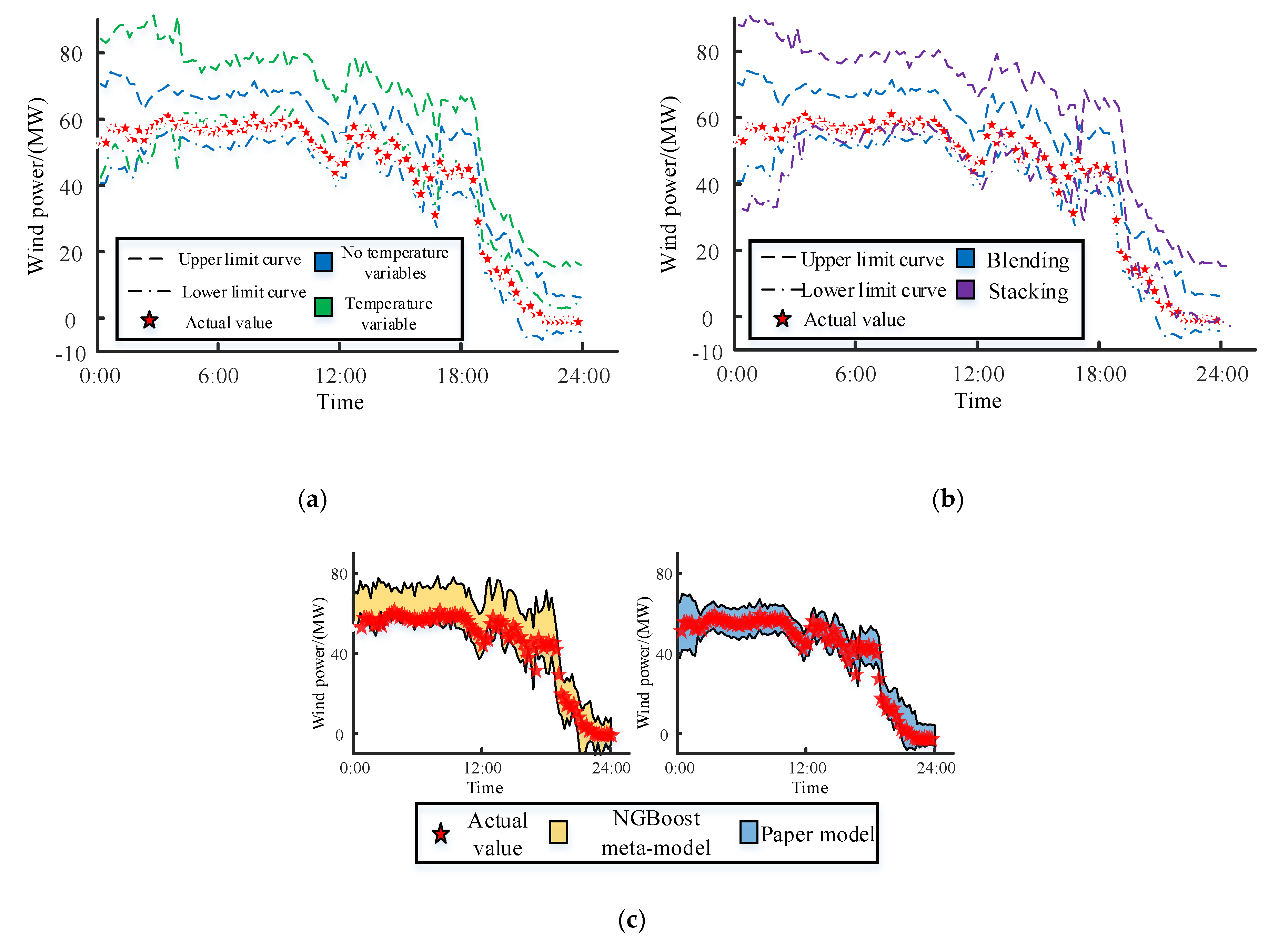
4.2.1. Effectiveness Analysis of Model Improvements

Different from the NGBoost metamodel proposed in the literature [33], the model proposed in this paper has the following innovations and improvements. (1) Data preprocessing is added. (2) Natural gradients are calculated through general gradients. (3) Blending fusion is used for strengthening the model training effect. In order to verify the effectiveness of the above improvements, based on the principle of controlled variables, we have conducted different experiments to prove the rationality and effectiveness of the improved model proposed in this paper. The visualization of the experimental results is shown in Figure 4.

The prediction effect is compared with and without data preprocessing drawn as shown in Figure 4a. It can be seen from Figure 4a that when the data set is not preprocessed, the abnormal data and weakly correlated input data represented by the temperature directly reduce the overall prediction level and the confidence of the prediction under the same confidence level. The interval shifted and expanded, which shows that weakly correlated data and outliers should not be used as training data for the model. The data preprocessing step added in this paper is reasonable and effective.

The fusion model comparison is shown in Figure 4b. It can be seen from Figure 4b that the stacking fusion that cannot overcome the problem of data traversal is not suitable for solving the probability prediction problem. Their prediction results have a large deviation. The blending fusion proposed in this paper exhibits better prediction performance in comparison.

The comparison of the model prediction effects between the improved NGBoost in this paper and the NGBoost metamodel proposed in [33] is shown in Figure 4c. It can be seen from Figure 4c that although the NGBoost proposed in document [33] has a good probability prediction effect, the prediction effect of the model proposed in this paper has been reinforced. It is better and more suitable for practical engineering applications for a short-term direct probability prediction of wind power.

The natural gradient calculation method proposed in the literature [33] and the calculation method proposed in this paper are used to calculate the data of the examples, respectively. Based on the evaluation indicators proposed in this paper, the calculation results under different confidence levels are shown in

Table 1. Model comparison data at different methods of natural gradient.

Confidence Level	Method of [33]			Method of This Paper
	IF (%)	IP (%)	IC	IF (%)	IP (%)	IC
80%	92.71	11.31	82.80	92.71	11.34	82.77
90%	96.88	12.11	82.14	96.88	12.07	82.17
95%	97.92	12.97	81.43	97.92	12.95	81.45

.

It can be seen from Table 1 that the natural gradient calculation method proposed in this paper is similar to the method proposed in the original text. However, the method in this paper can calculate the natural gradient through ordinary gradients which simplifies the calculation process and is obviously more suitable for a practical promotion and application in engineering situations than direct calculations.

4.2.2. Comparative Analysis with Other Models

In order to further illustrate the advantages of the improved NGBoost (model 1) proposed in this paper, the kernel extreme learning machine model (model 2) proposed in [40] and the naive Bayes combination model (model 3) proposed in [41] are selected as comparisons. The prediction results are evaluated according to the indicators proposed in Section 3. The comparison of the prediction confidence intervals of each model is shown in Figure 5. The index values of each model under different confidence levels are recorded in

Table 2. Models comparison at different confidence levels.

Confidence Level	Model 1			Model 2			Model 3
	IF (%)	IP (%)	IC	IF (%)	IP (%)	IC	IF (%)	IP (%)	IC
80%	93.75	7.81	86.71	43.75	32.36	31.60	81.25	38.22	55.34
90%	97.92	8.39	90.04	67.71	41.46	44.63	85.42	48.98	52.21
95%	98.96	9.55	89.95	72.92	49.55	44.32	88.54	58.53	49.17

.

It can be seen from Figure 5 and Table 2 that as the confidence level increases, the I_F of each model increases, and the I_P also gradually increases. Under the same confidence level, the I_F of model 1 is larger indicating that there is a smaller deviation in the mean of the prediction results. Similarly, the I_P of model 1 is larger than that of the models 2 and 3, representing that the sharpness of the prediction results is smaller. All in all, the model proposed in this paper can reduce I_P while ensuring a larger I_F and obtain a higher I_C. It exhibits a better performance in solving the probability prediction problem.

5. Conclusions

Aiming at the application defects of the NGBoost metamodel in solving the short-term direct probability prediction of wind power, this paper proposed an improved NGBoost model. The highlights of this model are the addition of data preprocessing avoiding the influence of abnormal data on the model prediction results and the use of general gradients to calculate natural gradients, simplifying the calculation process and facilitating the promotion of the model in practical engineering applications. What is more, this model includes the blending fusion strengthening of the model learning effect to obtain better prediction results. The effectiveness and advantages of the model proposed in this paper are verified by the measured data of Dalian Tuoshan wind farm in China. The following conclusions are drawn.

(1)

Considering actual engineering conditions, there are many outliers in the initial data set from SCADA in real wind farms which will cause final prediction errors. With the help of the box plot and gray correlation analysis proposed in this paper, the initial data set can be effectively preprocessed so that the model has a higher generalization and robustness.

(2)

The related concepts of direct calculation by natural gradients are extremely complicated, which is not conducive to popularization and applications in actual engineering. Based on the amount of Fisher information, calculating natural gradients through ordinary gradients is liable to simplify the metamodel calculation process and promote the model applicated in practical engineering.

(3)

Blending fusion is more suitable for solving probabilistic prediction problems effectively strengthening the learning effect of the metamodel without causing excessive model redundancy.

Based on the model proposed in this article, the subsequent research work that can be carried out includes: (1) the promotion and application of this model in other probabilistic forecasting fields, such as photovoltaics, load and so on. (2) The development of new energy integration based on the uncertainty information of wind power provided by this model into the research of power system scheduling optimization, new energy power market evaluation and other topics.

References

1. Huo, Y.; Jiang, P.; Zhu, Y.; Feng, S.; Wu, X. Optimal real-time scheduling of wind integrated power system presented with storage and wind forecast uncertainties. Energies 2015, 8, 1080–1100. [Google Scholar] [CrossRef]
2. Zuluaga, C.D.; Álvarez, M.A.; Giraldo, E. Short-term wind speed prediction based on robust Kalman filtering: An experimental comparison. Appl. Energy 2015, 156, 321–330. [Google Scholar] [CrossRef]
3. Neeraj, B.; Andrés, F.; Daniel, V.; Kulat, K. A novel and alternative approach for direct and indirect wind-power prediction methods. Energies 2018, 11, 2923. [Google Scholar]
4. Costa, A.; Crespo, A.; Navarro, J.; Lizcano, G.; Madsen, H.; Feitosa, E. A review on the young history of the wind power short-term prediction. Renew. Sustain. Energy Rev. 2008, 12, 1725–1744. [Google Scholar] [CrossRef] [Green Version]
5. Xie, L.; Gu, Y.; Zhu, X. Short-term patio-temporal wind power forecast in robust look-ahead power system dispatch. IEEE Trans. Smart Grid 2013, 5, 511–520. [Google Scholar] [CrossRef]
6. Buhan, S.; Özkazanç, Y.; Çadırcı, I. Wind pattern recognition and reference wind mast data correlations with NWP for improved wind-electric power forecasts. IEEE Trans. Ind. Inform. 2016, 12, 991–1004. [Google Scholar] [CrossRef]
7. Wei, W.; Zhang, Y.; Wu, G. Ultra-short-term/short-term wind power continuous prediction based on fuzzy clustering analysis. IEEE PES Innov. Smart Grid Technol. 2012, 7, 6. [Google Scholar] [CrossRef]
8. Sharma, K.C.; Jain, P.; Bhakar, R. Wind power scenario generation and reduction in stochastic programming framework. Electr. Power Compon. Syst. 2013, 41, 271–285. [Google Scholar] [CrossRef]
9. Ambach, D.; Croonenbroeck, C. A selection of time series models for short- to medium-term wind power forecasting. J. Wind Eng. Ind. Aerodyn. 2015, 136, 201–210. [Google Scholar]
10. Zhu, Q.; Chen, J.; Zhu, L.; Duan, X.; Liu, Y. Wind Speed Prediction with Spatio-temporal Correlation: A Deep Learning Approach. Energies 2018, 11, 705. [Google Scholar] [CrossRef] [Green Version]
11. Zheng, L.; Hu, W.; Min, Y. Raw wind data preprocessing: A data-mining approach. IEEE Trans. Sustain. Energy 2015, 6, 11–19. [Google Scholar] [CrossRef]
12. Khodayar, M.; Wang, J. Spatio-temporal graph deep neural network for short-term wind speed forecasting. IEEE Trans. Sustain. Energy 2019, 10, 670. [Google Scholar] [CrossRef]
13. Foley, A.M.; Leahy, P.G.; Marvuglia, A. Current methods and advances in forecasting of wind power generation. Renew. Energy 2012, 37, 1–8. [Google Scholar] [CrossRef] [Green Version]
14. Poncela, M.; Poncela, P.; Perán, J.R. Automatic tuning of Kalman filters by maximum likelihood methods for wind energy forecasting. Appl. Energy 2013, 108, 349–362. [Google Scholar] [CrossRef]
15. Zhang, Y.; Wang, P.; Zhang, C. Wind energy prediction with LS-SVM based on Lorenz perturbation. J. Eng. 2017, 13, 1724. [Google Scholar] [CrossRef]
16. Villacorta, C.; Cardoso, A.; Lima, C.G. Forecasting natural gas consumption using ARIMA models and artificial neural networks. IEEE Latin Am. Trans. 2016, 14, 2233. [Google Scholar] [CrossRef]
17. Zhu, Q.; Chen, J.; Shi, D.; Zhu, L.; Bai, X.; Duan, X.; Liu, Y. Learning Temporal and Spatial Correlations Jointly: A Unified Framework for Wind Speed Prediction. IEEE Trans. Sustain. Energy 2020, 11, 509–523. [Google Scholar] [CrossRef]
18. Yang, X.; Ma, X.; Kang, N. Probability interval prediction of wind power based on kde method with rough sets and weighted markov Chain. IEEE Access 2018, 6, 51556. [Google Scholar] [CrossRef]
19. Yu, R.; Liu, Z.; Li, X.; Lu, W.; Ma, D.; Yu, M.; Wang, J.; Li, B. Scene learning: Deep convolutional networks for wind power prediction by embedding turbines into grid space. Appl. Energy 2019, 238, 249–257. [Google Scholar] [CrossRef] [Green Version]
20. Yan, J.; Zhang, H.; Liu, Y.; Han, S.; Li, L. Uncertainty estimation for wind energy conversion by probabilistic wind turbine power curve modeling. Appl. Energy 2019, 239, 1356. [Google Scholar] [CrossRef]
21. Wan, C.; Xu, Z.; Pinson, P.; Dong, Z.Y.; Wong, K.P. Probabilistic forecasting of wind power generation using extreme learning machine. IEEE Trans. Power Syst. 2014, 29, 1033–1044. [Google Scholar] [CrossRef] [Green Version]
22. Naik, J.; Bisoi, R.; Dash, P.K. Prediction interval forecasting of wind speed and wind power using modes decomposition based low rank multi-kernel ridge regression. Renew. Energy 2018, 129, 357. [Google Scholar] [CrossRef]
23. Cui, M.; Krishnan, V.; Hodge, B.M.; Zhang, J. A copula-based conditional probabilistic forecast model for wind power ramps. IEEE Trans. Smart Grid 2018, 1, 13. [Google Scholar] [CrossRef]
24. Malvoni, M.; De Giorgi, M.G.; Congedo, P.M. Forecasting of PV Power Generation using weather input data-preprocessing techniques. Energy Procedia 2017, 126, 651. [Google Scholar] [CrossRef]
25. Zhang, G.Y.; Wu, Y.G.; Wong, K.P. An advanced approach for construction of optimal wind power prediction intervals. IEEE Trans. Power Syst. 2015, 30, 2706. [Google Scholar] [CrossRef]
26. Kou, P.; Liang, D.L.; Gao, F. Probabilistic wind power forecasting with online model selection and warped gaussian process. Energy Convers. Manag. 2014, 84, 649. [Google Scholar] [CrossRef]
27. Hu, M.Y.; Hu, Z.J.; Qian, M.L. Research on wind power prediction method based on improved AdaBoost. RT and KELM. Power Grid Technol. 2017, 41, 536. [Google Scholar]
28. He, D.; Wu, M. Probe into application of Ada-BP neural network improved algorithm in electric power load forecasting. Shanxi Electr. Power 2012, 40, 21–28. [Google Scholar]
29. Liu, W.; Zhang, R.F.; Peng, D.G. Load forecasting of distribution network based on k-adaboost data mining. Zhejiang Electr. Power 2019, 38, 104. [Google Scholar]
30. Tan, J.; Deng, C.H.; Yang, W. Ultra-short-term photovoltaic power forecasting in microgrid based on adaboost clustering. Autom. Electr. Power Syst. 2017, 41, 33. [Google Scholar]
31. Xie, C.Z.; Wang, J.C.; Xie, X.H. BOA-GBDT photovoltaic output prediction based on fine-grained features. Power Grid Technol. 2020, 44, 689. [Google Scholar]
32. Liu, B.; Qin, C.; Ju, P. Short-term bus load forecast based on the fusion of XGBoost and Stacking model. Electr. Power Autom. Equip. 2020, 40, 147. [Google Scholar]
33. Tony, D.; Anand, A.; Daisy, Y.D. NGBoost: Natural gradient boosting for probabilistic prediction. arXiv 2019, arXiv:1910.03225. [Google Scholar]
34. Zhang, Z.Z.; Zou, J.X.; Zheng, G. Ultra-short-term wind power prediction model based on modified grey model method for power control in wind farm. Wind Energy 2011, 35, 55. [Google Scholar] [CrossRef]
35. Han, Q.; Wu, H.; Hu, T.; Chu, F. Short-term wind speed forecasting based on signal decomposing algorithm and hybrid linear/nonlinear models. Energies 2018, 11, 2796. [Google Scholar] [CrossRef] [Green Version]
36. Dong, W.; Yang, Q.; Fang, X.L. Multi-step ahead wind power generation prediction based on hybrid machine learning techniques. Energies 2018, 11, 1975. [Google Scholar] [CrossRef] [Green Version]
37. Friedman, J.H. Greedy function approximation: A gradient boosting machine. Ann. Stat. 2001, 29, 1189–1232. [Google Scholar] [CrossRef]
38. Zhou, J.; Sun, N.; Jia, B.; Peng, T. A novel decomposition-optimization model for short-term wind speed forecasting. Energies 2018, 11, 1752. [Google Scholar] [CrossRef] [Green Version]
39. Meng, Y.H.; Zhi, J.H.; Jing, P.Y. A novel multi-objective optimal approach for wind power interval prediction. Energies 2017, 10, 419. [Google Scholar]
40. Huang, G.B. An insight into extreme learning machines: Random neurons, Random features and kernels. Cogn. Comput. 2014, 6, 376–390. [Google Scholar] [CrossRef]
41. Yang, X.Y.; Zhang, Y.F.; Ye, T.Z. Probabilistic interval prediction of wind power combination based on Naive Bayes. High Volt. Technol. 2020, 46, 1099. [Google Scholar]
Figure 1. Schematic diagram of Blending fusion.
Energies 13 04629 g001
Figure 2. Overall flow chart.
Energies 13 04629 g002
Figure 3. Data analysis charts. (a) original data visualization; (b) Box diagram of input weather variables; (c) Stacked histogram of input weather variables.
Energies 13 04629 g003
Figure 4. Improved model validity comparison verification. (a) Comparison with and without data preprocessing; (b) The fusion model comparison; (c) The comparison of model.
Energies 13 04629 g004
Figure 5. Models comparison.
Energies 13 04629 g005