Elastic and Frictional Properties of Fault Zones in Reservoir-Scale Hydro-Mechanical Models—A Sensitivity Study


Institut für Angewandte Geowissenschaften, TU Darmstadt, Schnittspahnstraße 9, 64287 Darmstadt, Germany
*
Author to whom correspondence should be addressed.
Energies 2020, 13(18), 4606; https://doi.org/10.3390/en13184606
Submission received: 4 August 2020
/
Revised: 31 August 2020
/
Accepted: 1 September 2020
/
Published: 4 September 2020
(This article belongs to the Special Issue Petroleum Geomechanics)
Abstract
:The proper representation of faults in coupled hydro-mechanical reservoir models is challenged, among others, by the difference between the small-scale heterogeneity of fault zones observed in nature and the large size of the calculation cells in numerical simulations. In the present study we use a generic finite element (FE) model with a volumetric fault zone description to examine what effect the corresponding upscaled material parameters have on pore pressures, stresses, and deformation within and surrounding the fault zone. Such a sensitivity study is important as the usually poor data base regarding specific hydro-mechanical fault properties as well as the upscaling process introduces uncertainties, whose impact on the modelling results is otherwise difficult to assess. Altogether, 87 scenarios with different elastic and plastic parameter combinations were studied. Numerical modelling results indicate that Young’s modulus and cohesion assigned to the fault zone have the strongest influence on the stress and strain perturbations, both in absolute numbers as well as regarding the spatial extent. Angle of internal friction has only a minor and Poisson’s ratio of the fault zone a negligible impact. Finally, some general recommendations concerning the choice of mechanical fault zone properties for reservoir-scale hydro-mechanical models are given.
1. Introduction
Hydro-mechanical simulations have developed into a standard tool for various subsurface applications ranging from hydrocarbon and geothermal reservoirs to underground storage sites for CO2 [1,2,3,4]. However, challenges exist regarding the proper implementation of faults into such numerical models. Faults not only have a profound impact on fluid flow, but also effect the stress field in their vicinity. In addition, pore pressure changes due to injection or production can induce slippage and fault reactivation, respectively [5,6,7,8]. This may cause induced seismicity, land subsidence and well collapse [9,10,11,12]. Fault reactivation may also breach the reservoir seal causing up-fault leakage and allowing fluid migration due to enhanced permeability inside the fault zone [13,14,15]. Thus, proper incorporation of faults into hydro-mechanical models is of crucial relevance for various reasons.
In reality, faults are characterized by a complex geometrical structure and a heterogeneous material distribution [16,17,18,19,20,21]. They should be regarded rather as a fault zone, i.e., a volumetric feature, than as a discrete fault surface [20,22,23,24]. A fault zone typically contains a fault core accompanied by damage zones on either side, but may be structurally more complex including the appearance of multiple fault cores as well as damage zones of variable width and fracture intensity [16,21,25,26,27]. Therefore, the appropriate representation of faults in numerical reservoir models is challenged by two related aspects: (1) the difference in scale between the heterogeneity of the fault zone (centimeters to meters) and the typical size of the calculation cells of the numerical grid (meters to tens of meters) and (2) the material properties assigned to the fault zone which stem—if available at all—from rock mechanical testing on core samples with a diameter of a few centimeters. Both aspects require upscaling, i.e., merging the heterogeneous material properties of the fault zone [28,29,30,31], in order to assign reasonable material properties to the fault zone elements of a reservoir-(kilometer)-scale hydro-mechanical model.
In the present study we use a generic finite element (FE) model with a volumetric fault zone description to examine what effect such upscaled parameters have on pore pressures, stresses, and deformation within and surrounding the fault zone. Such a sensitivity study is important as the usually poor data base regarding specific hydro-mechanical fault properties as well as the upscaling process introduces uncertainties, whose impact on the modeling results is otherwise difficult to assess. As the prime focus is on fault reactivation due to pore pressure changes, we explore a parameter range for Young’s modulus, Poisson’s ratio, cohesion, and angle of internal friction which is typical for fault zone rocks. Modeling results are expected to provide a framework to understand quantitatively how the elastic and frictional-plastic properties assigned to a fault zone in a hydro-mechanical reservoir simulation actually affect the modeling results.
2. Elastic and Frictional Fault Zone Properties
Faults are usually not a target for drilling operations. They are rather avoided to reduce well stability problems. Even if coring of a fault zone is attempted, intense fracturing and poor consolidation of fault zone rocks frequently results in very limited core recovery [32,33]. As a consequence, there usually is a lack of fault-specific material parameters to populate a hydro-mechanical model [34,35]. Instead, the material parameters have to be estimated from literature sources considering how faulting and fracturing change the material properties of the intact rock. In the following we review the possible range of mechanical fault rock parameters in the elastic and frictional-plastic domain, which also forms the basis for the subsequent numerical sensitivity study.
2.1. Elastic Material Properties
Deformation in the elastic domain can be described by Hooke’s Law, which relates stress and strain via an elasticity (or stiffness) matrix [36,37]. In case of a linear-elastic and isotropic medium, only two material properties are required: Young’s modulus and Poisson’s ratio. The Young’s modulus or modulus of elasticity of a fault zone can vary by several orders of magnitude between the value of the intact rock and the one of the fault-related rocks in the damage zones and fault core. The Young’s modulus for common lithologies (intact rock) ranges from 1 GPa to 100 GPa [24,38]. It decreases with increasing fracture density, i.e., in the damage zone and tectonic breccias, respectively. Fault gauges which frequently make up the fault core can exhibit Young’s modulus values as low as 0.01 GPa [24,39,40].
The Young’s modulus required for numerical modelling is the static Young’s modulus which—ideally—is derived from uniaxial or triaxial testing of cores in the laboratory. Such rock mechanical testing is typically carried out on samples with a diameter of a few centimeters. However, mechanical properties like Young’s modulus and unconfined compressive strength (UCS) derived from lab tests are usually significantly larger (1.5×–10×) than the corresponding values of a larger rock mass [24,37]. This scale-dependence can be accounted for by using empirical correlations, but this inevitably adds uncertainties to the material properties assigned to the fault zone in the numerical model [38,41,42]. If no cores are available, an option is to calculate dynamic Young’s modulus from well logs (p- and s-wave velocities, density). However, these dynamic Young’s modulus values need to be converted to static ones based on empirical correlations which introduces yet another uncertainty to the upscaled properties.
The second parameter to describe elasticity is Poisson’s ratio. It is defined as the negative transversal strain divided by the axial or longitudinal strain [24,43]. Again, determination of static Poisson’s ratio requires core samples for laboratory testing, while dynamic values can be derived from borehole logs (p- and s-wave velocities). Poisson’s ratios of common lithologies are usually in the range of 0.10–0.35 with most values between 0.2 and 0.3 [26,40,43]. If no specific measurements for the Poisson’s ratio of a rock unit is available, 0.25 is a value commonly used in numerical simulations.
2.2. Frictional Material Properties
In case of most rocks, elastic material behavior is restricted to only a few percent (1–3%) of deformation. If stresses reach the yield point, the subsequent post-failure behavior and irreversible deformation falls into the plastic domain [24,37,44]. In case of brittle-plastic material behavior, failure is realized through fracture formation, while in the ductile domain failure occurs as plastic flow [15,45,46]. Major crustal-scale fault zones include both failure mechanisms with fracturing and a well-defined fault zone in the upper part and plastic flow resulting in a distributed shear zone in the deeper part. However, at typical reservoir depths of a few kilometers, brittle failure is the dominant deformation mechanism in fault zones [47,48,49].
A commonly used failure criterion separating the elastic and the plastic domain is the Mohr–Coulomb (MC) failure criterion. The MC criterion defines the maximum shear stress a rock can withstand until shear failure occurs [34,43,50]. The corresponding frictional material properties of the MC criterion are cohesion and the angle of internal friction.
Cohesion, also called inherent shear strength, is the shear strength of a rock if the effective normal stress is zero [39,51,52]. The cohesion of fault zone rocks can vary by several orders of magnitude from completely cohesionless to a few tens of MPa depending on the degree of deformation and healing or recrystallization, e.g., from hydrothermal precipitations [15,26]. For example, a fault zone may contain a fully powdered fault core, which persists of cohesionless rock flour [16,20,22,53]. In contrast, circulation of hydrothermal fluids can cause mineral precipitation (e.g., quartz, barite), which hardens the fault core even more than the surrounding rock mass [18,52,54]. In order to estimate fault zone cohesion, some rules of thumb can be considered:
It should be noted that for sedimentary rocks the intercept of a linear Mohr–Coulomb criterion actually overestimates rock cement strength. In such cases, use of a nonlinear failure envelope would be more appropriate to describe real cohesion at low effective confining stresses.
The second frictional material parameter used in the MC criterion is the angle of internal friction. It describes the increase in shear strength of a rock with respect to an increase in normal stress [15,24,39]. Friction angles of common lithologies range between 5° and 50° [24,37]. A frequently used average value for rocks is 40.5° equivalent to a coefficient of internal friction of 0.85 [50]. In general, the friction angle is related to grain size, so coarse-grained rocks tend to have a higher friction angle, while lower friction angles are typical for fine-grained rocks and rocks with a high clay content, respectively [57,58,59,60,61]. Besides grain size, the degree of fracturing also affects the angle of internal friction [62]. Typically, the friction angle decreases with increasing fracturing of the rock [63,64].
However, other studies [65,66] indicate that during rock degradation in shear and without further weakening due to mineral alteration and clay smearing, the friction angle remains largely unaltered. Thus, weakening in such cases results primarily from cohesion softening.
A fault-specific determination of cohesion and angle of internal friction again requires core samples for triaxial rock mechanical testing in the lab. If the material is not suitable for multistage testing [67,68,69], at least three samples are required for one triaxial test. Thus, it is very rare that proper rock samples for triaxial testing of fault zone rocks are available to populate a numerical model with specific frictional fault rock properties [15,24].
3. Modelling Concept
A finite element (FE) model was set up to compare the effect on hydro-mechanical simulation of different elastic and frictional-plastic properties assigned to a fault zone. It consists of over and underburden sections of low permeability with a high-permeability reservoir layer in between and offset by a normal fault. Figure 1a exhibits an elliptical fault zone displacing a reservoir horizon, the geological rationale for this model setup. The reservoir horizon embedded into the 1 km × 1 km × 0.003 km model frame is displaced by a 500 m long normal fault centered in the middle of the model. At the top of the model frame, loading conditions simulate 1 km of overlaying rock material. So the model bottom is adopted to be 2 km beneath the surface. Additionally, the weight of the overburden implemented as pressure acting on the model top, no further mechanical forces, or displacements are assigned to the model. On the hydraulic part, the initial model assumes a hydrostatic pore pressure field. Subsequently, pore pressure at the nodes on the right side of the reservoir unit is increased to simulate fluid injection into the downthrown block. For five years the pore pressure is constantly increased every three months by 0.75 MPa until it finally reaches 15 MPa above hydrostatic.
Starting from a base model which is used as reference for the subsequent sensitivity studies, Young’s modulus, Poisson’s ratio, cohesion, and angle of internal friction are varied within a range typical for fault zone rocks. At the same time, the model geometry and the material properties for the other model units (reservoir rock and over-/underburden) remain the same in all scenarios. Altogether, 87 FE models with different mechanical parameter combinations assigned to the fault zone have been studied. FE software Ansys 19.2 [70] is used for the fully coupled hydro-mechanical simulations.
3.1. Model Geometry
The 3D model represents a slice through the central part of a normal fault (Figure 1a). The resulting model domain, the dimensions as well as the initial and boundary conditions are shown in Figure 1b. The model dimensions are 1 km × 1 km × 0.001 km (equivalent to a model slice of one element thickness) and comprise a fault zone of 500 m height and 60° dip. The fault offsets a 25 m thick reservoir section by 47 m. Using scaling relationships of Johri et al. [33], the total width of the fault zone including the fault core as well the damage zone is assumed to be 12 m. Treffeisen and Henk [71] have shown that in reservoir-scale models discretizing the width of a fault zone into three elements is sufficient to achieve modelling results very similar to a finer discretization. Hence, the size of the elements describing the fault geometry is 4 m × 4 m × 3 m, whereas the whole model domain comprises 45,684 elements.
3.2. Constitutive Laws
The hydro-mechanical simulation uses fluid flow through a porous medium and poroelastic-perfectly plastic material behavior. In the following the principle behind such fully coupled hydro-mechanical simulations as well as the assigned boundary conditions are briefly explained. The Modelling utilizes the commercial software program Ansys 19.2 and the reader is referred to the extensive theory and user manuals [70] for more detailed information.
The mechanical part of the fully coupled simulation is based on the total stresses are reduced by the pore pressure in the rock volume leading to effective stresses. This relationship can be described by [72,73,74]:
where the effective stresses (σ′ij) are derived from the total stress tensor (σij) by subtracting the pore pressure (pf), weighted by the Biot coefficient (α) and Kronecker’s delta (δij).
σ′ij = σij – α ∙ pf ∙ δij
The hydraulic part of the coupling is defined in Ansys 19.2 with the following mass-balance equation [70]:
where the flux due to Darcy’s law qf (m/s), the volumetric strain εv (-), the compressibility parameter Q* and the degree of fluid saturation Sf (-). Q* is calculated from the bulk modulus of both the skeleton and the fluid.
3.3. Initial and Boundary Conditions
Figure 1b shows the mechanical and hydraulic boundary conditions, both for the initial state and the subsequent injection stage. For the mechanical calculations, displacements orthogonal to the model boundaries are not allowed at the base, left, right, front, and back sides of the model (roller boundary conditions). Since the model top is located 1000 m beneath the earth surface, the weight of the overburden is assigned through a pressure boundary condition with an average density of 2300 kg/m3. For the hydraulic calculations, all model boundaries are considered to be impermeable.
During the initial load step, mechanical and hydraulic equilibrium in response to the boundary conditions is achieved. So the whole model domain experiences hydrostatic pore pressure conditions. Concurrently the initial stress field is established through gravitational loading only and no other tectonic (horizontal) stress components are considered in the simulations. Therefore, the tectonic regime is normal faulting with the vertical stress Sv being the maximum principal stress S1.
Afterwards, fluid injection in the downthrown block is simulated by successively applying higher pore pressures for five years to the boundary nodes of the reservoir layer in the hanging wall of the fault (lower right in Figure 1b). The injection pressure increases for 20 time steps by 0.75 MPa, until the maximum injection pressure of 15 MPa above hydrostatic is reached.
3.4. Material Parameters
The hydraulic and mechanical material properties assigned to the fault zone, reservoir and host rock are listed in Table 1. Details of the changes in Young’s modulus, Poisson’s ratio, cohesion, and friction angle assigned to the fault zone in the various sensitivity studies as well as the acronyms dedicated to the corresponding scenarios are shown in Table 2. The coding used for each model variant reflects the differences to the base model (BM). For example, BM-c1 implies that the model varies only regarding cohesion of the fault zone rocks and that a value of 1 MPa (instead of 5 MPa as in model BM) is used for the calculations. All other material parameters remain the same.
The material properties assigned to the fault zone elements cover a range which is typical for fault zones in siliciclastic successions, i.e., Young’s modulus was varied between 0.01 GPa and 10 GPa, Poisson’s ratio between 0.1 and 0.25, cohesion between 0.01 MPa and 5 MPa and friction angle between 10.0° and 25.0°. For example, the combination of the maximum values from each category, e.g., a Young’s modulus of 10 GPa, a Poisson’s ratio of 0.25, a cohesion of 5 MPa and a friction angle of 25°, would be typical for a fault zone containing slightly deformed sandstone and re-cemented fault gouge [15,24,39]. Combination of the minimum values, i.e., a Young’s modulus of 0.01 GPa, a Poisson’s ratio of 0.1, a cohesion of 0.01 MPa and a friction angle of 10° would represent a fault rock containing mostly clay and siliciclastic rock flour [26]. Between these extremes, various other rock types and, hence, material properties can be imagined, depending on the fraction clay or rock and the fraction of lithified sandstone [43].
The permeability of fault zones in siliciclastic successions is usually controlled by the clay content of the offset rocks. Thus, impermeable faults are more likely in sandstone-shale regimes [16,59,75]. However, we decided to choose a semipermeable fault zone since we are particularly interested in how fluid flow effects the mechanical strength of the fault and how this potentially leads to fault reactivation [2,15]. Faults in sandstones with less than 15% clay content show already a slightly reduced permeability in comparison to the host rock [76]. For this sensitivity study, we choose a fault zone permeability about two orders of magnitude lower than the reservoir rock to account for some fault damage on hydraulic conductivity. However, modelling techniques are generally applicable and could also be applied to fault zones which act as impermeable barriers or high-permeability conduits for fluid flow.
4. Results
The following section presents some of the modeling results. Firstly, the results of the base model (BM) are presented, which provides the baseline for the following comparisons with some of the other 86 scenarios studied (see Table 2 for the various models). Afterwards stress and strain patterns for both the whole model area and the fault zone itself are compared between exemplary model setups.
4.1. Base Model
The base model (BM) comprises a fault zone with material properties typical for siliciclastic fault zones separating a sandstone reservoir, whereby the fault acts as conduit for fluid flow between different reservoir compartments. The corresponding mechanical material properties for a fault zone in such a setting are inferred from literature [24,40,43] and set to a Young’s modulus of 10 GPa, a Poisson’s ratio of 0.25, a cohesion of 10 MPa and an angle of internal friction of 25°. Modelling results are illustrated in Figure 1 and Figure 2 comparing the results for the initial state, i.e., prior to fluid injection (upper row) and after five years of injection with a pore pressure increase in the lower reservoir section of 15 MPa above hydrostatic (bottom row), respectively.
4.1.1. Pore Pressure
The initial pore pressure distribution (Figure 2a) shows a hydrostatic gradient resulting from the boundary conditions assigned, i.e., 9.8 MPa at the model top (1000 m depth) and 19.6 MPa at the model base (2000 m). After increasing the injection pressure at a rate of 0.75 MPa every three month over five years to a total of 15 MPa above hydrostatic, the pore pressure inside the reservoir layer has been raised to 30 MPa (Figure 2d). The pressure increase has propagated from the injection point in the down-thrown reservoir section through the fault zone all the way up to the upper fault compartment on the left side of the model. The increase here is still about 8 MPa above hydrostatic, which results in a pore pressure of about 22 MPa.
4.1.2. Magnitude and Orientation of S1,eff
The effective maximum principal stress (S1,eff) displays 15 MPa at the top and up to 37 MPa at the bottom of the model (Figure 2b). This reflects the combined effects of boundary conditions and gravitational loading and considers poroelastic effects. The fault zone shows the lowest effective stress values due to its higher Biot coefficient in comparison to the surrounding rock mass. Figure 2c displays the orientation of S1,eff. For ease of visualization, this is presented in form of a contour plot which show the deviations (clockwise (CW) and counterclockwise (CCW)) from the vertical direction, i.e., the undisturbed orientation of S1,eff in a normal faulting regime. As a consequence, outside the model areas affected by the fault hardly any deviation occurs, i.e., S1,eff is vertical. However, inside the fault zone S1,eff has rotated up to 17° CW. In the immediate vicinity of the fault zone and near the fault tips, stress rotations between 5° CCW and 5° CW can be observed.
After five years of fluid injection the pore pressure inside the reservoir (Figure 2d) and the fault zone has increased which directly effects the S1,eff pattern (Figure 2e). The lower, right reservoir section stands out against the surrounding rock mass with S1,eff values about 5–10 MPa lower, while the effective stresses near the fault zone show an increase at the upper left and lower right fault tips as well as a corresponding decrease at the opposing sides. Inside the fault zone, S1,eff has decreased up to less than 10 MPa. Injection does not only modify effective stress magnitudes but also stress orientations (Figure 2f). Significantly larger model areas up to 300 m distance from the fault zone are now showing S1,eff orientations differing from vertical. These stress perturbations follow some kind of a point symmetry with a maximum rotation of 21° CW to the left of the lower and to the right of the upper fault tip, respectively. On the opposite sides of the fault tips extending to the middle part of the fault zone, the direction of S1,eff deviates between 5° and 15° CW from vertical.
4.1.3. Total, Elastic, and Plastic Strain
Figure 3 shows the von Mises total strain as well as the corresponding elastic and plastic strain components. For the first load step, total strain ranges from 0 to 0.16% (Figure 3a) and is dominated by elastic straining (compare to Figure 3b,c). After five years of injection, the total strain exhibits values between 0.0 and 1.6% (Figure 3d) and is primarily controlled by plastic straining, which shows significantly higher values than the elastic strain component (compare to Figure 3e,f). Elastic straining only in relation to the initial stress field is shown in Figure 3b. In the vicinity of the fault zone von Mises elastic strain values range from 0.04% at the top to 0.1% at base. Somewhat larger strain values are observed for the weaker fault zone where values range between 0.12% and 0.16%. These lower elastic strains are confined to the fault zone and do not extend into the surrounding rock mass. No von Mises plastic strain is observed for the initial load step (Figure 3c). Thus, it can be excluded that initial loading already causes plastic deformation in and reactivation of the fault zone. For the final load step, i.e., after five years of injection, elastic strain in the fault zone has decreased by about 0.04% compared to the initial load step, ranging now between 0.08% and 0.12% (Figure 3e). The larger elastic strain values extend into the surrounding host rock at the fault tips. While elastic strain has decreased inside the fault zone, plastic strain has increased and occurs throughout the entire fault zone (Figure 3f). Maximum values are about 1.6% at the fault tips, but even within the fault zone plastic straining of at least 0.5% can be observed.
4.2. Influence of Young’s Modulus
Comparison of the various sensitivity studies starts with the elastic domain and by varying the Young’s modulus assigned to the fault zone elements. Three scenarios differing by an order of magnitude, i.e., 10 GPa, 1 GPa, and 0.1 GPa, are compared. The remaining fault zone properties, i.e., Poisson’s ratio, cohesion and friction angle are kept constant at 0.25, 5 MPa, and 25°, respectively.
4.2.1. Magnitude and Orientation of S1,eff
Figure 4a–c show the magnitude of S1,eff after five years of fluid injection for the three different Young’s modulus values of the fault zone. Figure 4a shows the results of the base model (BM). S1,eff magnitudes to the right of the lower and to the left of the upper fault tip are 43.7 MPa and 32.3 MPa, respectively. On the opposite sides, there are local minima of 17.9 MPa and 24.8 MPa. The lowest values for S1,eff of 7.6 MPa can be observed in the central part of the fault zone. A decrease in Young’s modulus to 1 GPa (BM-Y1) does not change this overall pattern of S1,eff with minimum and maximum peaks at the fault tips arranged point symmetric to the midpoint of the fault (Figure 4b). However, the maximum values at the lower and upper fault tips are 59.6 MPa and 48.3 MPa, respectively. Thus, the less stiffer fault zone leads to an increase in S1,eff magnitudes by about 16 to 17 MPa in comparison to the base model. The local minima opposite those peaks are 14.2 and 25.6 MPa, respectively. Again, the lowest values of 2.83 MPa can be found in the central part of the fault. A further decrease of the Young’s modulus of the fault zone to 0.1 GPa (model BM-Y0.1) intensifies these trends even more (Figure 4c). The maximum values at the fault tips range between 68.6 MPa and 85.7 MPa and the local minimum between 8.7 MPa and 17.4 MPa. The lowest S1,eff magnitudes of 0.3 MPa are again observed in the middle of the fault zone.
The corresponding orientation of S1,eff for the three scenarios with different fault zone Young’s modulus values are presented in Figure 4d–f. After five years of fluid injection, most parts of the base model (BM) show only minor (5° CCW to 5° CW) deviations from vertical (Figure 4d). Larger values of up to 20° CW occur near the right side at the upper and the left side of the lower fault tip. On the opposing sides and towards the center of the fault zone CCW rotation up to 13.7° is observed. A decrease in Young’s modulus to 1 GPa (BM-Y1) increases both the area affected by and the amount of stress rotation (Figure 4e), while the overall pattern remains the same. The maximum rotation of 33.5° CW occurs to the right of the upper and to the left of the lower fault tip, while on the opposing sides a deviation from vertical of up to 21.4° CCW is observed. The further decrease of the Young’s modulus to 0.1 GPa (BM-Y0.1, Figure 4f) enhances this pattern leading to stress rotations between 48.4° CW and 32.0° CCW.
4.2.2. Elastic and Plastic Strain
The impact of different fault zone Young’s modulus values on elastic and plastic strain patterns after five years of injection is shown in Figure 5. Model BM shows a maximum elastic strain of 0.12% in the fault zone elements (Figure 5a; see also Figure 3e which uses a different color scale to visualize details). Decreasing Young’s modulus by a factor of 10 (BM-Y1), the maximum values for the elastic strain inside the fault zone is increased to 1.03% (Figure 5b). A further decrease in Young’s modulus (BM-Y0.1) leads to larger elastic strain values observed in the fault zone especially at the fault tips, where values can reach up to 7.8% (Figure 5c). Such high elastic strain values can only be achieved because the frictional properties are kept constant in this comparison.
The results for the plastic strain appear to be the other way around (Figure 5d–f). Model BM seems to show plastic straining primarily in the lower part of the fault zone (Figure 5d). However, Figure 3f, which uses a different color contour scheme, shows, that plastic straining actually occurs throughout the entire fault zone with a peak value of 1.5% at the lower fault tip. In model BM-Y1, no through-going plastic strain zone has developed, but the strain peak at the lower fault tip is about twice as much with 3.06% (Figure 5e). For BM-Y0.1 the plastic strain is limited to only a very small area at the lower fault tip, where the maximum value is 1.02% (Figure 5f). The remaining part of the fault zone does not experience any plastic straining.
4.3. Influence of Poisson’s Ratio
4.3.1. Magnitude and Orientation of S1,eff and S2,eff
The effect of different Poisson’s ratios of the fault zone rocks on the magnitude of both the vertical (S1,eff) and horizontal (S2,eff) effective stress is shown in Figure 6. The pattern of S1,eff magnitudes after five years of fluid injection is essentially the same for all scenarios i.e., for Poisson’s ratios of 0.25 (BM, Figure 6a), 0.15 (BM-P0.15, Figure 6b), and 0.10 (BM-P0.10, Figure 6c). The minimum values inside the fault zone hardly vary for the three models, ranging between 7.4 MPa (BM) and 7.5 MPa (BM-P0.10). Maximum values observed at the lower fault tips vary from 43.7 (BM) to 45.8 (BM-P0.10).
Comparing the results of S2,eff the overall pattern is again rather similar with peak values in the range of 12 MPa. However, some differences occur inside the fault zone, where minimum S2,eff values are 1.3 MPa (BM, Figure 6d), 0.8 MPa (BM-P0.15, Figure 6e), and 0.5 MPa (BM-P0.10, Figure 6f), respectively.
Regarding the orientation of S1,eff and S2,eff, the calculated patterns exhibit no substantial differences depending of the Poisson’s ratio assigned to the fault zone unit.
4.3.2. Elastic and Plastic Strain
Figure 7 combines elastic and plastic strain results received for the different Poisson’s ratio values assigned to the fault zone. The elastic strain pattern and the peak values of 0.13% are essentially the same for all three models (Figure 7a–c). Plastic straining also shows a comparable pattern restricted to the fault zone with maximum values of 1.54%, 1.73%, and 1.76% for models BM, BM-P0.15, and BM-P0.10, respectively (Figure 7d–f).
4.4. Influence of Cohesion
4.4.1. Magnitude and Orientation of S1,eff
Different patterns of S1,eff magnitudes derived after five years of fluid injection are compared in Figure 8a–c for three different cohesion values assigned to the fault zone elements. The values vary from 5 MPa (BM), through 0.5 MPa (BM-c0.5) to 0.01 (BM-c0.01) MPa, while all other fault zone material properties remain the same. Modelling results for BM regarding the magnitude of S1,eff are pictured in Figure 8a, which shows the maximum of 43.7 MPa at the lower fault tip and the minimum of 7.5 MPa inside the fault zone. For a decrease in cohesion to 0.5 MPa (BM-c0.5) the local maximum at the fault tip increases to 59.1 MPa, while the minimum in the middle of the fault decreases to 2.7 MPa (Figure 8b). If the cohesion is decreased even further (BM-c0.01) the corresponding values are 60.5 MPa and 2.7 MPa, respectively (Figure 8c).
Comparing the different results (Figure 8d–f) received for the orientation of S1,eff, similar trends can be observed. Model BM exhibits a CW rotation of S1,eff from the vertical orientation of about 20.0° right at the upper left of the lower fault tip extending up to 15 m parallel to the fault into the host rock (Figure 8d). A CCW rotation of 13.7° can be observed on the opposite side of each fault tip, ranging more towards the middle of the fault and extending up to 20 m parallel into the host rock. Changing cohesion to 0.5 MPa (BM-c0.5) enlarges the areas affected by stress rotation as well as the maximum rotation achieved (Figure 8e). S1,eff deviations from vertical in the vicinity of the fault zone range from to 36.5° CW to 22.9° CCW and extent for up to 50 m into the host rock. A further decrease in cohesion to 0.01 MPa (BM-c0.01) only very slight increases the spatial extent of these stress perturbations and the range is now between 37.8° CW and 24.3° CCW (Figure 8f).
4.4.2. Elastic and Plastic Strain
As has been described above for model BM, elastic strain inside the fault zone ranges between 0.08% and 0.12%, with the maximum being at 0.13% at the lower fault tip (Figure 9a). Decreasing cohesion to 0.5 MPa (BM-c0.5), the elastic strain pattern changes to a certain extent (Figure 9b). Instead of showing the highest values inside the fault zone like in model BM, the values inside the fault zone are the lowest of the whole model domain with a minimum of 0.02%. The maxima remain at the fault tips and increase further to a maximum of 0.16%. A further decrease in cohesion to 0.01 MPa (BM-c0.01) does not change this basic pattern and only slight modifies the values for the minimum within the fault zone and the maximum at the fault tips to 0.01% and 0.17%, respectively (Figure 9c).
The corresponding plastic strain pattern after five years of injection is presented in Figure 9d–f. Due to the color contour scheme required to compare the various simulation results, model BM seems to show plastic strain only in a small area near the base of the fault zone (Figure 9d). However, the detailed analysis shown in Figure 3f reveals that plastic straining actually occurs in the entire fault zone. Plastic strain varies between 0.31% and 0.62% throughout the fault zone and reaches a maximum of 1.54% at the lower fault tip. For a decrease in cohesion to 0.5 MPa (BM-c0.5), the values inside the fault zone increase to 0.81% to 1.61% with a local maximum at the lower fault tip of 4.03% (Figure 9e). A further decrease in cohesion to 0.01 MPa (BM-c0.01) increases the maximum peak to 4.43%, but within the fault zone itself, the values only increase to between 0.89% and 1.77%. However, the basic plastic strain pattern remains the same (Figure 9f).
4.5. Influence of Friction Angle
4.5.1. Magnitude and Orientation of S1,eff
The influence of the angle of internal friction of the fault zone rocks is investigated by comparing the modelling results after five years of injection for scenarios with friction angles of 25.0°, 17.5°, and 10.0°. All other properties are kept constant. The basic pattern regarding the magnitude of S1,eff is similar in all three cases and shows local maxima near the fault tips and minimum values inside the fault zone. For model BM the corresponding values are 43.7 MPa and 7.5 MPa, respectively (Figure 10a). A decrease of the friction angle to 17.5° (BM-FA17.5) increases the difference between these extremes (Figure 10b). The maximum S1,eff magnitude of 48.1 MPa is observed at the lower fault tip, while it is only 7.1 MPa inside the fault zone. A further decrease of the friction angle to 10.0° (BM-FA10) intensifies this difference even more and the corresponding values are 52.3 MPa and 6.6 MPa, respectively (Figure 10c).
Regarding the orientation of S1,eff, Figure 10d shows the results of model BM after five years of fluid injection into the reservoir. Orientations deviate from vertical up to 20.0° CW to the right of the upper and to the left of the lower fault tip. The opposing sides of the fault zone show a CCW rotation of 13.7°. Deviations of more than 2.5° from vertical are confined to the immediate vicinity of the fault (up to 70 m). For scenario BM-FA17.5 modeling results show an increase in both the area affected by stress rotations as well as the rotation angles (Figure 10e). The deviations from vertical range between 25.5° CW and 14.4° CCW, extending up to 85 m into the vicinity of the fault. This trend continues if the friction angle of the fault zone is reduced to 10.0° (BM-FA10, Figure 10f). Stress perturbations now extent up to 100 m into the host rock of the fault zone and stress rotations vary between 29.7° CW and 15.6° CCW.
4.5.2. Elastic and Plastic Strain
Regarding elastic strain, modeling shows rather similar results for the three different friction angles. There are only minor differences in the strain distribution within the fault zone and the maximum values reached. Model BM model exhibits values up to 0.09%–0.1% in large parts of the fault zone, whereas the peak value of 0.13% is confined to a small area near the lower fault tip (Figure 11a). For model BM-FA17.5, the elastic strain observed inside the fault zone decreases to 0.08%–0.09% (Figure 11b), but the area affected by higher elastic strains in continuation of the fault both updip and downdip is enlarged. This trend continues for a friction angle to 10.0° (BM-FA10) for which elastic strain within the fault zone is reduced to 0.07%–0.08% (Figure 11c), while the area affected by elastic straining in the vicinity of the fault zone widens.
Considering plastic strain, the trend is reverse. Instead of a decrease in fault zone straining with a decrease in friction angle as was the case for elastic strain, plastic strain within the fault zone increases with decreasing angle of internal friction of the fault rock. Model BM shows plastic strain values of less than 0.4% in most parts of the fault zone (Figure 11d) and a maximum of 1.54% at the lower fault tip. BM-FA17.5 exhibits plastic strain within the fault zone of up to 0.8% (Figure 11e) and to 2.07% at the lower fault tip. Both values increase even further in BM-FA10 to 1.0% plastic strain within the fault zone and 2.61% (Figure 11f).
4.6. Interdependence of Parameters
4.6.1. Elastic Properties (Young’s Modulus vs. Poisson’s Ratio)
The impact of different elastic fault zone material properties on the simulation results after five years of fluid injection are examined by analyzing twelve scenarios with different Young’s modulus and Poisson’s ratios, respectively. Figure 12 shows the maximum values calculated for each model regarding the magnitude of S1,eff, elastic and plastic strain plotted against the Young’s modulus for different Poisson’s ratios. All three plots indicate that the different curves, each representing a specific Poisson’s ratio, are very close, especially for the magnitude of S1,eff and the elastic strain (Figure 12a,b). Only for plastic strain they differ between 1.0% and 1.75% for a Young’s modulus of 0.1 GPa.
A large influence on the modelling results can be observed for Young’s modulus. Considering Figure 12a, the magnitude of S1,eff decreases by 20 to 25 MPa if the Young’s modulus increases about one order of magnitude. In addition, elastic strain shows decreasing maximum values for increasing Young’s moduli (Figure 12b). However, plastic strain results are different as illustrated in Figure 12 c. It shows the maximum elastic, plastic, and total strain values for different Young’s moduli. At first, plastic strain increases with increasing Young’s modulus until a maximum value of about 3.4% is reached for a Young’s modulus of 0.5 GPa. From that point on plastic strain decreases with further increasing fault zone Young’s modulus until maximum plastic straining is 1.75% for a Young’s modulus of 10 GPa (Figure 12c). At the same time, elastic straining reaches its minimum. However, even though the maximum values at the fault tips differ, the general pattern within the fault zone proper remains the same: increasing Young’s modulus lead to larger plastic strain observed in the fault zone.
4.6.2. Plastic Properties (Cohesion vs. Internal Friction Angle)
The impact of the plastic properties assigned to the fault is assessed by analyzing 12 scenarios with different parameter combinations of cohesion and angle of internal friction. For this comparison, the maximum values for the magnitude of S1,eff and plastic strain achieved in the model domain are plotted against cohesion for different angles of internal friction (Figure 13). Both the magnitude of S1,eff and the plastic strain show only a small reduction with increasing cohesion as long as cohesion is less than 1 MPa. For example, the maximum values of the magnitude of S1,eff achieved for variations in the cohesion of the base model (Figure 13a) are 60.51 MPa (BM-c0.01), 59.14 MPa (BM-c0.5), and 57.84 MPa (BM-c1) until the values for S1,eff drop significantly to 43.72 MPa (BM) for 5 MPa cohesion. The same behavior can be observed for plastic strain (Figure 13 b), where the values are 4.43% (BM-c0.01), 4.03% (BM-c0.5) and 3.74% (BM-c1) before decreasing to 1.54% (BM). In both graphs of Figure 13, the distances between the curves derived for various internal friction angles are the same. Thus, for a constant cohesion value, the maximum S1,eff magnitude and the maximum plastic strain decrease linearly with an increase in friction angle.
Although the maximum values partially differ significantly, the general modeling results are rather similar for variations in cohesion and internal friction angle. In Figure 14 the stress pattern for the magnitude of S1,eff is shown as an example and similar trends can be observed in orientation plots as well. The base model with its rock properties is displayed in Figure 14a. The rows display the different results achieved for a constant cohesion value by varying the internal friction angle from left (25°) to right (10°) and the columns show the results for one specific friction angle while varying the cohesion from top (5 MPa) to bottom (0.01 MPa). An increase in both the peak magnitude of S1,eff as well as the spatial extent of the stress perturbation can be observed for a decrease in friction angle as well as a decrease in cohesion. Apart from the stress peaks at the fault tips, the effect of varying the internal friction angle on the overall stress pattern is not visible at all and the differences can be only observed at the peak values located at the fault tips.
5. Discussion
Firstly, the base model (BM) is evaluated to ensure proper model behavior and, building on that, the modelling results for different material properties inside the fault zone are discussed.
5.1. Base Model
The BM results for pore pressure (Figure 2a) and S1,eff magnitudes outside the areas affected by the fault zone show the expected increase with depth resulting from the different fluid and rock densities (Figure 2b). The S1,eff orientation in these areas is vertical and thus, in agreement with the normal faulting regime [77] induced by the prescribed boundary conditions (Figure 2c). The fault zone is not reactivated as a result of initial loading as no plastic straining (Figure 3c) and no differential displacements are observed. After five years of fluid injection into the lower reservoir section, fluid migration through the fault zone has also led to an increase in pore pressure in the upper reservoir part (Figure 2d). More importantly, the pore pressure increase within the fault zone has reduced the effective stresses (Figure 2e), thus, leading to plastic straining (Figure 3f) and reactivation of the fault as well as differential displacements along its entire length. This fault reactivation has also modified the stress magnitudes (Figure 2e) and orientations (Figure 2f) in the vicinity of the fault zone. Comparable patterns regarding spatial extent and magnitude of the stress changes have also been reported from other numerical simulations of faults [5,14,78].
5.2. Variations in Elastic Rock Properties
Comparison of the scenarios which differ with respect to Young’s modulus shows that a decrease in Young’s modulus assigned to the fault zone leads to an increase in the magnitude and re-orientation of S1,eff as well as the spatial extent of the stress perturbations (Figure 4). Thus, this relationship follows a negative correlation. For example, the models evaluated in Section 4.2.1 show for BM, BM-Y1, and BM-Y0.1 that the magnitude and the rotation angle of S1,eff increases if the Young’s modulus of the fault zone is decreased. These trends for Young’s modulus can also be observed if combined with other material properties like different Poisson’s ratios, cohesions, and internal friction angles. Thus, stiffness contrasts between the fault represented as volumetric weak zone and the host rock lead to magnitude changes as well as stress rotations. Softer rock properties in the fault zone lead to a larger stiffness contrast with respect to the surrounding, which results in broader ranges of between maxima and minima for S1,eff magnitudes and stress reorientations, respectively [79,80]. Similarly, the spatial extent of the stress perturbations increases with decreasing stiffness of the fault zone and increasing stiffness contrast, respectively.
The stiffness contrast between the fault zone and the surrounding rock mass also affects the strain values observed in the fault zone. A larger stiffness contrast and therefore a broader ranges of S1,eff magnitudes results in larger values of total strain (Figure 12c). With increasing Young’s modulus in the fault zone and, hence, a reduction in stiffness contrast to the country rock, the total strain decreases.
The different Young’s moduli imply different slopes of the curves in the stress-strain diagram. Thus, for a given failure stress lower Young’s moduli result in larger elastic deformation prior to failure or, in other words, for a given amount of total deformation the share of plastic deformation is less in case of lower Young’s modulus. These trends are supported by the modelling results, i.e., peak S1,eff magnitude, elastic strain as well as total strain decrease with increasing Young’s modulus of the fault zone rocks. Likewise, the plastic strain should increase with increasing Young’s modulus, which is the case for Young’s modulus between 0.1 and 0.5 GPa. However, the maximum value is observed for a Young’s modulus of 0.5 GPa and the maximum plastic strain decreases between a Young’s modulus of 0.5 and 10 GPa (Figure 12c). Thus, the total strain decrease in response to a Young’s modulus increase delimits the maximum plastic strain which is achieved in response to respective stress states. The elastic strain component reaches its maximum at a low fault zone stiffness, whereas at high fault zone stiffnesses total strain is dominated by plastic straining.
Contrary to the large influence Young’s modulus has on the modelling results, the Poisson’s ratio assigned to the fault zone appears to have a negligible impact. This is somewhat surprising as under gravitational loading only Poisson’s ratio relates the horizontal stress SH (MPa) to the vertical stress SV (MPa) according to [37]:
Although this relationship holds for the rock units surrounding the fault zone, changing Poisson ratio ν (-) inside the fault zone (while keeping it constant in the rest of the model) has hardly any impact onto the modelling results. The effect of different Poisson’s ratios inside the fault zone on the stress and strain pattern is apparently suppressed by the influence the Poisson’s ratio of the surrounding rock mass has on the overall stress and strain patterns.
5.3. Variations in Plastic Rock Properties
If elastic fault zone properties are kept constant and only frictional-plastic material parameters are varied, modeling results are rather similar as long as cohesion is less than 1 MPa (Figure 8 and Figure 9). For larger cohesion values, a substantial drop in both the magnitude of S1,eff and plastic strain is observed (Figure 13). The increase in pore pressure and the corresponding decrease in effective stresses within the fault zone shifts the Mohr circle in the Mohr–Coulomb diagram towards the failure line and results, in case of lower cohesion values, in larger plastic straining. In turn, larger plastic straining and fault reactivation leads to a stronger loading of the vicinity of the fault and, hence, larger S1,eff magnitudes. For the modeling scenario selected in this study with gravitational loading only, a cohesion of 1 MPa appears to be some kind of a threshold value at larger cohesion values substantially less fault reactivation occurs resulting in reduced stress perturbations concerning both magnitude and spatial extent.
If cohesion is kept constant, the internal friction angle shows a negative correlation for all result parameters. Thus, an increase in the internal friction angle decreases the magnitude and rotation angle of the effective maximum principal stress (S1,eff) as well as the values for maximum elastic and plastic strain. This, again, can be explained by the Mohr–Coulomb diagram: the larger the friction angle and, hence, the steeper the slope of the failure line is, the more differential stress the fault zone rock can stand prior to failure. Thus, more stress states are in the plastic domain if the friction angle is lower which in turn results in stronger stress perturbations again.
Differences in the overall pattern for both stress and strain can hardly be detected and the results only seem to differ at the fault tips (Figure 10, Figure 11, and Figure 13). In reality however a fault usually does not end within the reservoir and therefore the area of interest in reservoir modelling, hence the effects of that only occur within a few meters at the fault tips and are not important in reservoir engineering.
6. Conclusions
Using a simple generic model setup of a normal fault offsetting a reservoir horizon, the impact of different mechanical fault properties on the stress and strain distribution within a fault zone and its surrounding is analyzed. Thereby, the fault is represented as a volumetric weak zone with uniform properties which inherently implies upscaling of the small-scale heterogeneity of faults observed in nature as well as of the limited size of lab samples available for mechanical testing to the large cell size of the reservoir-scale hydro-mechanical model. This study provides insights on how the elastic and plastic material properties assigned to fault zones of a reservoir-scale model actually affect the results of the numerical simulation. Therefore, it helps to choose proper upscaled fault zone properties by knowing the effect each mechanical parameter has.
Starting with a base model as reference, the mechanical properties assigned to the fault zone are varied within a range typical for faults in sandstone-shale successions, i.e., Young’s modulus between 0.1 and 10 GPa, Poisson’s ratio between 0.10 and 0.25, cohesion between 0.01 and 5 MPa and angle of internal friction between 10° and 25°. Altogether, 87 different scenarios were studied. Modelling results indicate that these four material properties have substantially different influences on the stress and strain perturbations induced by the fault. The Young’s modulus of the fault zone and, more specifically, the contrast in Young’s modulus between fault zone and surrounding rocks has by far the strongest impact onto the modelling result. The larger the difference in Young’s modulus is, the larger the stress and strain perturbations are, both in absolute numbers as well as regarding the spatial extent. Cohesion turns out to be the second most important material property. In comparison to these two parameters, the impact of the internal friction angle is minor and of the Poisson’s ratio assigned to the fault zone essentially negligible.
Consequently, the following guidelines for modelling of faulted reservoirs can be derived from this sensitivity study: If the stress and strain patterns in the vicinity of faults, i.e., within a few hundred meters, are not in the focus of the particular modelling project, the fault zone properties can be determined based on literature data and/or rules of thumb as outlined in Chapter 2. This holds because modelling results indicate that the exact fault properties have no impact on the stress and strain distribution in the far-field of the fault. This, however, changes in the vicinity of a reservoir-scale fault zone, i.e., within a few hundred meters distance to the fault.
If this near-field of a fault is of interest for the modeling study, the reservoir simulation workflow has to start with a first guess of the fault zone parameters based on literature data and experience as usually only very limited or no fault-specific material parameters are available. The initial model run should then be followed by an iterative calibration process by comparing the simulation results to data actually observed. These could be stress orientations (e.g., from borehole breakouts and drilling-induced fractures observed in image logs) and/or stress magnitudes (e.g., from hydraulic tests) observed in wells in the vicinity of the fault. According to the results of the present sensitivity study, during the calibration process the modeler can focus on Young’s modulus and cohesion as the most important parameters to achieve a satisfactory fit between model predictions and reality. These two properties are the crucial parameters to assess the reactivation potential of a fault as well as the stress and strain patterns in its vicinity. The angle of internal friction is of less relevance and for Poisson’s ratio the standard value of 0.25 can be adopted without concern. This reduction in the number of variables to be tuned during calibration substantially reduces time and computational costs to achieve a validated fault zone description for the hydro-mechanical reservoir model.
This sensitivity studies cannot provide quantitative relationships between the parameters since too many variables besides the four material properties studied influence fault response in hydro-mechanical models. For example, different elastic properties in over and underburden relative to the fault zone would lead to variable stiffness contrast in different sections of the fault zone. This, in turn, would affect the stress and strain patterns in the vicinity of the fault.
However, this sensitivity study provides a guideline which material properties should be of prime interest during upscaling and model calibration. This is also valid, if local mesh refinement in the reservoir-scale model is performed in order to capture the geometrical heterogeneity of the fault zone in greater detail and with smaller elements, respectively. Perspectives for future modelling work include highly detailed fault zone models to provide a sound physical base for upscaling of hydro-mechanical material parameters.
Author Contributions
Conceptualization: T.T.; data curation: T.T.; formal analysis: T.T.; funding acquisition: A.H.; investigation: T.T.; methodology: T.T.; project administration: A.H.; resources: T.T.; software: T.T.; supervision: A.H.; validation: T.T.; visualization: T.T.; writing—original draft: T.T.; writing—review and editing: A.H. Both authors have read and agreed to the published version of the manuscript.
Funding
We acknowledge support by the German Research Foundation and the Open Access Publishing Fund of Technical University of Darmstadt. This research received no further external funding. The research was financed from the unrestricted-use budget of the chair of Engineering Geology from TU Darmstadt. It did not receive funding from agencies in the public, commercial, or not-for-profit sectors.
Acknowledgments
We thank Dominik Gottron, Cord-Gerrit Peters and Karsten Reiter for helpful discussions regarding elasto-plastic material properties and modelling results during various parts of this research. Three anonymous reviewers are thanked for their helpful comments and constructive criticism on an earlier version of the manuscript.
Conflicts of Interest
The authors declare no conflict of interest.
Nomenclature
| α | Biot coefficient |
| c | Cohesion |
| E | Young’s modulus |
| k | Permeability |
| pf | Pore pressure |
| qf | Fluid flux due to Darcy’S law |
| Q* | Compressibility parameter |
| Sf | Degree of fluid saturation |
| S1,eff | Effective maximum principal stress |
| S2,eff | Horizontal effective stress |
| T0 | Tensile strength |
| v | Poisson’s ratio |
| εv | Volumetric strain |
| φ | Internal friction angle |
| σij | Total stress tensor |
| σ′ij | Effective stress tensor |
| δij | Kronecker’s delta |
| ρ | Density |
References
- Cappa, F.; Rutqvist, J. Modeling of coupled deformation and permeability evolution during fault reactivation induced by deep underground injection of CO2. Int. J. Greenh. Gas Control 2011, 5, 336–346. [Google Scholar] [CrossRef] [Green Version]
- Fachri, J.T.M.; Røe, P. Volumetric faults in field-sized reservoir simulation models: A first case study. AAPG Bull. 2016, 100, 795–817. [Google Scholar] [CrossRef]
- Serajian, V.; Diessl, J.; Bruno, M.S.; Hermansson, L.C.; Hatland, J.; Risanger, M.; Torsvik, R.M. 3D geomechanical modeling and fault reactivation risk analysis for a well at brage oilfield, norway. In Proceedings of the SPE Europec Featured at 78th EAGE Conference and Exhibition, Vienna, Austria, 30 May–2 June 2016. [Google Scholar]
- Schuite, J.; Longuevergne, L.; Bour, O.; Burbey, T.J.; Boudin, F.; Lavenant, N.; Davy, P. Understanding the hydromechanical behavior of a fault zone from transient surface tilt and fluid pressure observations at hourly time scales. Water Resour. Res. 2017, 53, 10558–10582. [Google Scholar] [CrossRef] [Green Version]
- Pereira, L.C.; Guimarães, L.J.; Horowitz, B.; Sánchez, M. Coupled hydro-mechanical fault reactivation analysis incorporating evidence theory for uncertainty quantification. Comput. Geotech. 2014, 56, 202–215. [Google Scholar] [CrossRef]
- Rueda, J.C.; Norena, N.V.; Oliveira, M.F.F.; Roehl, D. Numerical models for detection of fault reactivation in oil and gas fields. In Proceedings of the 48th US Rock Mechanics/Geomechanics Symposium, Minneapolis, Minnesota, 1–4 June 2014. [Google Scholar]
- Sanchez, E.C.; Zegarra, E.; Oliveira, M.F.F.; Roehl, D. Application of a 2D equivalent continuum approach to the assessment of geological fault reactivation in reservoirs. In Proceedings of the XXXVI Ibero-Latin American Congress on Computational Methods in Engineering, Rio de Janeiro, Brazil, 22–25 November 2015. [Google Scholar]
- Haug, C.; Nüchter, J.-A.; Henk, A. Assessment of geological factors potentially affecting production-induced seismicity in North German gas fields. Géoméch. Energy Environ. 2018, 16, 15–31. [Google Scholar] [CrossRef]
- Segall, P.; Grasso, J.-R.; Mossop, A. Poroelastic stressing and induced seismicity near the Lacq gas field, southwestern France. J. Geophys. Res. Space Phys. 1994, 99, 15423. [Google Scholar] [CrossRef]
- Morton, R.A.; Bernier, J.C.; Barras, J.A. Evidence of regional subsidence and associated interior wetland loss induced by hydrocarbon production, Gulf Coast region, USA. Environ. Earth Sci. 2006, 50, 261–274. [Google Scholar] [CrossRef]
- Chan, A.W.; Zoback, M.D. The role of hydrocarbon production on land subsidence and fault reactivation in the Loiusiana Coastal Zone. J. Coast. Res. 2007, 24, 771–786. [Google Scholar] [CrossRef]
- Vilarrasa, V.; Makhnenko, R.; Laloui, L. Potential for fault reactivation due to CO2 injection in a semi-closed saline aquifer. Energy Procedia 2017, 114, 3282–3290. [Google Scholar] [CrossRef] [Green Version]
- Wiprut, D.; Zoback, M.D. Fault reactivation and fluid flow along a previously dormant normal fault in the northern North Sea. Geology 2000, 28, 595–598. [Google Scholar] [CrossRef]
- Cuisiat, F.; Jostad, H.P.; Andresen, L.; Skurtveit, E.; Skomedal, E.; Hettema, M.; Lyslo, K. Geomechanical integrity of sealing faults during depressurization of the Statfjord field. J. Struct. Geol. 2010, 32, 1754–1767. [Google Scholar] [CrossRef]
- Faulkner, D.R.; Jackson, C.; Lunn, R.J.; Schlische, R.; Shipton, Z.K.; Wibberley, C.; Withjack, M. A review of recent developments concerning the structure, mechanics and fluid flow properties of fault zones. J. Struct. Geol. 2010, 32, 1557–1575. [Google Scholar] [CrossRef]
- Caine, J.S.; Evans, J.P.; Forster, C.B. Fault zone architecture and permeability structure. Geology 1996, 24, 1025–1028. [Google Scholar] [CrossRef]
- Walsh, J.J.; Bailey, W.; Childs, C.; Nicol, A.; Bonson, C. Formation of segmented normal faults: A 3-D perspective. J. Struct. Geol. 2003, 25, 1251–1262. [Google Scholar] [CrossRef]
- Collettini, C.; Holdsworth, R. Fault zone weakening and character of slip along low-angle normal faults: Insights from the Zuccale fault, Elba, Italy. J. Geol. Soc. 2004, 161, 1039–1051. [Google Scholar] [CrossRef]
- Myers, R.; Aydin, A. The evolution of faults formed by shearing across joint zones in sandstone. J. Struct. Geol. 2004, 26, 947–966. [Google Scholar] [CrossRef]
- Childs, C.; Manzocchi, T.; Walsh, J.J.; Bonson, C.G.; Nicol, A.; Schöpfer, M.P.J. A geometric model of fault zone and fault rock thickness variations. J. Struct. Geol. 2009, 31, 117–127. [Google Scholar] [CrossRef]
- Fasching, F.; Vanek, R. Engineering geological characterization of fault rocks and fault zones. Geomech. Tunn. 2011, 4, 181–194. [Google Scholar] [CrossRef]
- Rawling, G.C.; Goodwin, L.B.; Wilson, J.L. Internal architecture, permeability structure, and hydrologic significance of contrasting fault-zone types. Geology 2001, 29, 43–46. [Google Scholar] [CrossRef]
- Wibberley, C.A.J.; Yielding, G.; Di Toro, G. Recent advances in the understanding of fault zone internal structure: A review. Geol. Soc. Lond. Spéc. Publ. 2008, 299, 5–33. [Google Scholar] [CrossRef] [Green Version]
- Gudmundsson, A. Rock Fractures in Geological Processes by Agust Gudmundsson; Cambridge University Press (CUP): Cambridge, UK, 2009. [Google Scholar]
- Childs, C.; Watterson, J.; Walsh, J.J. A model for the structure and development of fault zones. J. Geol. Soc. 1996, 153, 337–340. [Google Scholar] [CrossRef]
- Gudmundsson, A.; De Guidi, G.; Scudero, S. Length–displacement scaling and fault growth. Tectonophysics 2013, 608, 1298–1309. [Google Scholar] [CrossRef]
- Bauer, J.F.; Meier, S.; Philipp, S.L. Architecture, fracture system, mechanical properties and permeability structure of a fault zone in Lower Triassic sandstone, Upper Rhine Graben. Tectonophysics 2015, 647, 132–145. [Google Scholar] [CrossRef]
- Manzocchi, T.; Heath, A.E.; Palananthakumar, B.; Childs, C.; Walsh, J.J. Faults in conventional flow simulation models: A consideration of representational assumptions and geological uncertainties. Pet. Geosci. 2008, 14, 91–110. [Google Scholar] [CrossRef]
- Olden, P.; Pickup, G.E.; Jin, M.; Mackay, E.J.; Hamilton, S.; Somerville, J.; Todd, A. Use of rock mechanics laboratory data in geomechanical modelling to increase confidence in CO2 geological storage. Int. J. Greenh. Gas Control 2012, 11, 304–315. [Google Scholar] [CrossRef]
- Zhang, Y.; Langhi, L.; Schaubs, P.; Piane, C.D.; Dewhurst, D.N.; Stalker, L.; Michael, K. Geomechanical stability of CO2 containment at the South West Hub Western Australia: A coupled geomechanical–fluid flow modelling approach. Int. J. Greenh. Gas Control. 2015, 37, 12–23. [Google Scholar] [CrossRef]
- Qu, D.; Tveranger, J. Incorporation of deformation band fault damage zones in reservoir models. AAPG Bull. 2016, 100, 423–443. [Google Scholar] [CrossRef] [Green Version]
- Paul, P.K.; Zoback, M.D.; Hennings, P.H. Fluid flow in a fractured reservoir using a geomechanically constrained fault-zone-damage model for reservoir simulation. SPE Reserv. Eval. Eng. 2009, 12, 562–575. [Google Scholar] [CrossRef] [Green Version]
- Johri, M.; Zoback, M.D.; Hennings, P. A scaling law to characterize fault-damage zones at reservoir depths. AAPG Bull. 2014, 98, 2057–2079. [Google Scholar] [CrossRef] [Green Version]
- Zoback, M. Reservoir Geomechanics; Cambridge University Press: Cambridge, UK, 2007. [Google Scholar]
- Hennings, P.; Allwardt, P.; Paul, P.; Zahm, C.; Reid, R.; Alley, H.; Kirschner, R.; Lee, B.; Hough, E. Relationship between fractures, fault zones, stress, and reservoir productivity in the Suban gas field, Sumatra, Indonesia. AAPG Bull. 2012, 96, 753–772. [Google Scholar] [CrossRef]
- Carmichael, R.S. Practical Handbook of Physical Properties of Rocks and Minerals (1988); Informa UK Limited: London, UK, 2017. [Google Scholar]
- Jaeger, J.; Cook, N.G.; Zimmerman, R. Fundamentals of Rock Mechanics, 4th ed.; Wiley-Blackwell: Hoboken, NJ, USA, 2007. [Google Scholar]
- Fjær, E. Relations between static and dynamic moduli of sedimentary rocks. Geophys. Prospect. 2018, 67, 128–139. [Google Scholar] [CrossRef] [Green Version]
- Goodman, R.E. Introduction to Rock Mechanics, 2nd ed.; Wiley: New York, NY, USA, 1989. [Google Scholar]
- Schön, J.H. Physical Properties of Rocks—Fundamentals of Petrophysics; Elsevier: London, UK, 2004. [Google Scholar]
- Eissa, E.A.; Kazi, A. Relation between static and dynamic Young’s moduli of rocks. Int. J. Rock Mech. Min. Sci. Geomech. 1988, 25, 479–482. [Google Scholar] [CrossRef]
- Davarpanah, S.M.; Ván, P.; Vásárhelyi, B. Investigation of the relationship between dynamic and static deformation moduli of rocks. Géoméch. Geophys. Geo Energy Geo Resour. 2020, 6, 1–14. [Google Scholar] [CrossRef] [Green Version]
- Fjær, E.; Holt, R.; Horsrud, P.; Raaen, A.; Risnes, R. Petroleum Related Rock Mechanics, 2nd ed.; Elsevier Science: Amsterdam, The Netherlands, 2008; pp. 103–133. [Google Scholar]
- Brady, B.H.G.; Brown, E.T. Rock Mechanics for Underground Mining, 2nd ed.; Kluwer: London, UK, 1993. [Google Scholar]
- Brace, W.F. An extension of the Griffith theory of fracture to rocks. J. Geophys. Res. Space Phys. 1960, 65, 3477–3480. [Google Scholar] [CrossRef]
- Caddell, R.M. Deformation and Fracture of Solids; Prentice-Hall: Upper Saddle River, NJ, USA, 1980. [Google Scholar]
- Reches, Z.; Lockner, D.A. Nucleation and growth of faults in brittle rocks. J. Geophys. Res. Space Phys. 1994, 99, 18159–18173. [Google Scholar] [CrossRef]
- Hoek, E. Practical Rock Engineering, 2nd ed.; Hoek’s Corner: North Vancouver, BC, Canada, 2013. [Google Scholar]
- Deb, R.; Jenny, P. Modeling of shear failure in fractured reservoirs with a porous matrix. Comput. Geosci. 2017, 21, 1119–1134. [Google Scholar] [CrossRef]
- Byerlee, J. Friction of rocks. Pageoph 1978, 116, 615–626. [Google Scholar] [CrossRef]
- Bell, F.G. Engineering Properties of Soils and Rocks, 4th ed.; Blackwell: Oxford, UK, 2000. [Google Scholar]
- Azarfar, B.; Peik, B.; Abbasi, B. A discussion on numerical modeling of fault for large open pit mines. In Proceedings of the 52th US Rock Mechanics/Geomechanics Symposium, Seattle, WA, USA, 17–20 June 2018. [Google Scholar]
- Holdsworth, R.E. Weak Faults—Rotten Cores. Science 2004, 303, 181–182. [Google Scholar] [CrossRef]
- Syversveen, A.R.; Skorstad, A.; Soleng, H.H.; Røe, P.; Tveranger, J. Facies modelling in fault zones. In Proceedings of the ECMOR X—10th European Conference on the Mathematics of Oil Recovery, Amsterdam, The Netherlands, 4–7 September 2006; pp. 4–7. [Google Scholar]
- Hoek, E.; Martin, C. Fracture initiation and propagation in intact rock–A review. J. Rock Mech. Geotech. Eng. 2014, 6, 287–300. [Google Scholar] [CrossRef] [Green Version]
- Bruhn, R.L.; Parry, W.T.; Yonkee, W.A.; Thompson, T. Fracturing and hydrothermal alteration in normal fault zones. Pure Appl. Geophys. Pageoph 1994, 142, 609–644. [Google Scholar] [CrossRef]
- Barton, N. Review of a new shear-strength criterion for rock joints. Eng. Geol. 1973, 7, 287–332. [Google Scholar] [CrossRef]
- Andersson, J.-E.; Ekman, L.; Nordqvist, R.; Winberg, A. Hydraulic testing and modelling of a low-angle fracture zone at Finnsjön, Sweden. J. Hydrol. 1991, 126, 45–77. [Google Scholar] [CrossRef]
- Faulkner, D.R.; Mitchell, T.M.; Healy, D.; Heap, M.J. Slip on ’weak’ faults by the rotation of regional stress in the fracture damage zone. Nature 2006, 444, 922–925. [Google Scholar] [CrossRef] [PubMed]
- Chiaraluce, L.; Chiarabba, C.; Collettini, C.; Piccinini, D.; Cocco, M. Architecture and mechanics of an active low-angle normal fault: Alto tiberina fault, northern Apennines, Italy. J. Geophys. Res. Space Phys. 2007, 112, 112. [Google Scholar] [CrossRef]
- Collettini, C.; Niemeijer, A.R.; Viti, C.; Marone, C. Fault zone fabric and fault weakness. Nature 2009, 462, 907–910. [Google Scholar] [CrossRef]
- Małkowski, P. Behaviour of joints in sandstones during the shear test. Acta Geodyn. Geomater. 2015, 12, 399–410. [Google Scholar] [CrossRef] [Green Version]
- Sanetra, U. The change of internal friction angle of intact and jointed rock on different depth. In Proceedings of the Mining Workshops, Polska Akademia Nauk, Wydawnictwo, Kraków, Poland, 15–18 June 2005. [Google Scholar]
- Bukowska, M.; Sanetra, U. The tests of the conventional triaxial granite and dolomite compression in the aspect of their mechanical properties. Min. Resour. Manag. 2008, 24, 345–358. [Google Scholar]
- Sulem, J.; Vardoulakis, I.; Papamichos, E.; Oulahna, A.; Tronvoll, J. Elasto-plastic modelling of Red Wildmoor sandstone. Mech. Cohes. Frict. Mater. 1999, 4, 215–245. [Google Scholar] [CrossRef]
- Jafarpour, M.; Rahmati, H.; Azadbakht, S.; Nouri, A.; Chan, D.; Vaziri, H. Determination of mobilized strength properties of degrading sandstone. Soils Found. 2012, 52, 658–667. [Google Scholar] [CrossRef] [Green Version]
- Bro, A. Analysis of multistage triaxial test results for a strain-hardening rock. Int. J. Rock Mech. Min. Sci. 1997, 34, 143–145. [Google Scholar] [CrossRef]
- Blümel, M. Comparison of single and multiple failure triaxial tests. In Proceedings of the ISRM Regional Symposium—EUROCK 2009, Cavtat, Croatia, 29–31 October 2009; pp. 239–242. [Google Scholar]
- Taheri, A.; Chanda, E. A new multiple-step loading triaxial test method for brittle rocks. In Proceedings of the 19th NZGS Geotechnical Symposium, Queenstown, New Zealand, 21–22 November 2013. [Google Scholar]
- Ansys Inc. Ansys 19.2; Ansys Inc.: Canonsburg, PA, USA, 2019. [Google Scholar]
- Treffeisen, T.; Henk, A. Faults as volumetric weak zones in reservoir-scale hydro-mechanical finite element models—A comparison based on grid geometry, mesh resolution and fault dip. Energies 2020, 13, 2673. [Google Scholar] [CrossRef]
- Wang, H.F. Theory of Linear Poroelasticity—With Applications to Geomechanics and Hydrogeology; Princeton University Press: Princeton, NY, USA, 2000. [Google Scholar]
- Shapiro, S. Fundamentals of Poroelasticity. In Fluid-Induced Seismicity; Shapiro, S., Ed.; Cambridge University Press: Cambridge, UK, 2015; pp. 48–117. [Google Scholar]
- Cheng, A.H.-D. Poroelasticity; Springer Science and Business Media LLC: Berlin, Germany, 2016; Volume 27. [Google Scholar]
- Agosta, F.; Prasad, M.; Aydin, A. Physical properties of carbonate fault rocks, fucino basin (Central Italy): Implications for fault seal in platform carbonates. Geofluids 2007, 7, 19–32. [Google Scholar] [CrossRef]
- Fisher, Q.J.; Knipe, R. The permeability of faults within siliclastic petroleum reservoirs of the North Sea and Norwegian Continental Shelf. Mar. Pet. Geol. 2001, 18, 1063–1081. [Google Scholar] [CrossRef]
- Anderson, E.M. The Dynamics of Faulting and Dyke Formation with Application to Britain, 2nd ed.; Oliver and Boyd: Edinburgh, UK, 1951. [Google Scholar]
- De Souza, A.L.S.; De Souza, J.A.B.; Meurer, G.B.; Naveira, V.P.; Chaves, R.A.P. Reservoir reomechanics study for deepwater field identifies ways to maximize reservoir performance while reducing geomechanics risk. In Proceedings of the SPE Asia Pacific Oil and Gas Conference, Perth, Australia, 22–24 October 2012. [Google Scholar]
- Bell, J.S. In situ stresses in sedimentary rocks (part 2): Applications of stress measurements. Geosci. Can. 1996, 23, 135–153. [Google Scholar]
- Zhang, Y.-Z.; Dusseault, M.B.; Yassir, N.A. Effects of rock anisotropy and heterogeneity on stress distributions at selected sites in North America. Eng. Geol. 1994, 37, 181–197. [Google Scholar] [CrossRef]
Figure 1.
(a) A slice through a reservoir horizon displaced by the central part of an elliptical fault zone is the geological rationale for the 3D fault zone model as shown in the cartoon. (b) General model set-up for the hydro-mechanical simulations as well as initial and boundary conditions used.
Figure 1.
(a) A slice through a reservoir horizon displaced by the central part of an elliptical fault zone is the geological rationale for the 3D fault zone model as shown in the cartoon. (b) General model set-up for the hydro-mechanical simulations as well as initial and boundary conditions used.

Figure 2.
Results of the base model (BM) of the spatial variation in pore pressure (a,d), the magnitude of the effective maximum principal stress (S1,eff; b,e), and orientation of S1,eff (deviation from vertical; c,f).
Figure 2.
Results of the base model (BM) of the spatial variation in pore pressure (a,d), the magnitude of the effective maximum principal stress (S1,eff; b,e), and orientation of S1,eff (deviation from vertical; c,f).

Figure 3.
Strain simulation results for the base model (BM), i.e., the spatial variation in von Mises total strain (a,d), von Mises elastic strain (b,e), and von Mises plastic strain (c,f).
Figure 3.
Strain simulation results for the base model (BM), i.e., the spatial variation in von Mises total strain (a,d), von Mises elastic strain (b,e), and von Mises plastic strain (c,f).

Figure 4.
Spatial variations in the magnitude (a–c) and orientation (deviation from vertical; d–f) of the effective maximum principal stress (S1,eff) after five years of injection for three different Young’s modulus values assigned to the fault zone.
Figure 4.
Spatial variations in the magnitude (a–c) and orientation (deviation from vertical; d–f) of the effective maximum principal stress (S1,eff) after five years of injection for three different Young’s modulus values assigned to the fault zone.

Figure 5.
Spatial variations in van Mises elastic (a–c) and plastic (d–f) strain after five years of injection for three different Young’s modulus values assigned to the fault zone.
Figure 5.
Spatial variations in van Mises elastic (a–c) and plastic (d–f) strain after five years of injection for three different Young’s modulus values assigned to the fault zone.

Figure 6.
Spatial variations in the magnitude of S1,eff (a–c) and the magnitude of S2,eff (d–f) after five years of injection for three different Poisson’s ratios assigned to the fault zone.
Figure 6.
Spatial variations in the magnitude of S1,eff (a–c) and the magnitude of S2,eff (d–f) after five years of injection for three different Poisson’s ratios assigned to the fault zone.

Figure 7.
Spatial variations in the van Mises elastic (a–c) and plastic strain (d–f) after five years of injection for three different Poisson’s ratios assigned to the fault zone.
Figure 7.
Spatial variations in the van Mises elastic (a–c) and plastic strain (d–f) after five years of injection for three different Poisson’s ratios assigned to the fault zone.

Figure 8.
Spatial variations in the magnitude (a–c) and orientation (deviation from vertical; d–f) of the effective maximum principal stress (S1,eff) after five years of injection for three different cohesion values assigned to the fault zone.
Figure 8.
Spatial variations in the magnitude (a–c) and orientation (deviation from vertical; d–f) of the effective maximum principal stress (S1,eff) after five years of injection for three different cohesion values assigned to the fault zone.
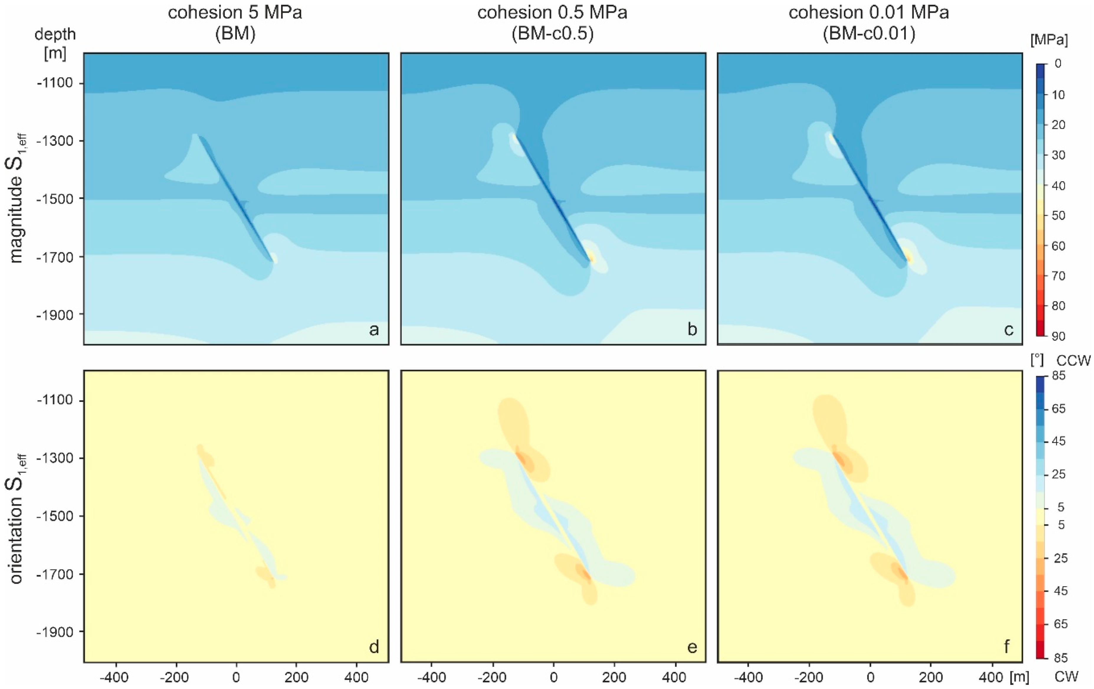
Figure 9.
Spatial variations in the van Mises elastic (a–c) and plastic strain (d–f) after five years of injection for three different cohesion values assigned to the fault zone.
Figure 9.
Spatial variations in the van Mises elastic (a–c) and plastic strain (d–f) after five years of injection for three different cohesion values assigned to the fault zone.

Figure 10.
Spatial variation in the magnitude (a–c) and the orientation (deviation from vertical; d–f) of the effective maximum principal stress (S1,eff) after five years of injection for three different friction angles assigned to the fault zone.
Figure 10.
Spatial variation in the magnitude (a–c) and the orientation (deviation from vertical; d–f) of the effective maximum principal stress (S1,eff) after five years of injection for three different friction angles assigned to the fault zone.

Figure 11.
Spatial variations in the van Mises elastic (a–c) and plastic (d–f) strain after five years of injection for three different friction angles assigned to the fault zone.
Figure 11.
Spatial variations in the van Mises elastic (a–c) and plastic (d–f) strain after five years of injection for three different friction angles assigned to the fault zone.
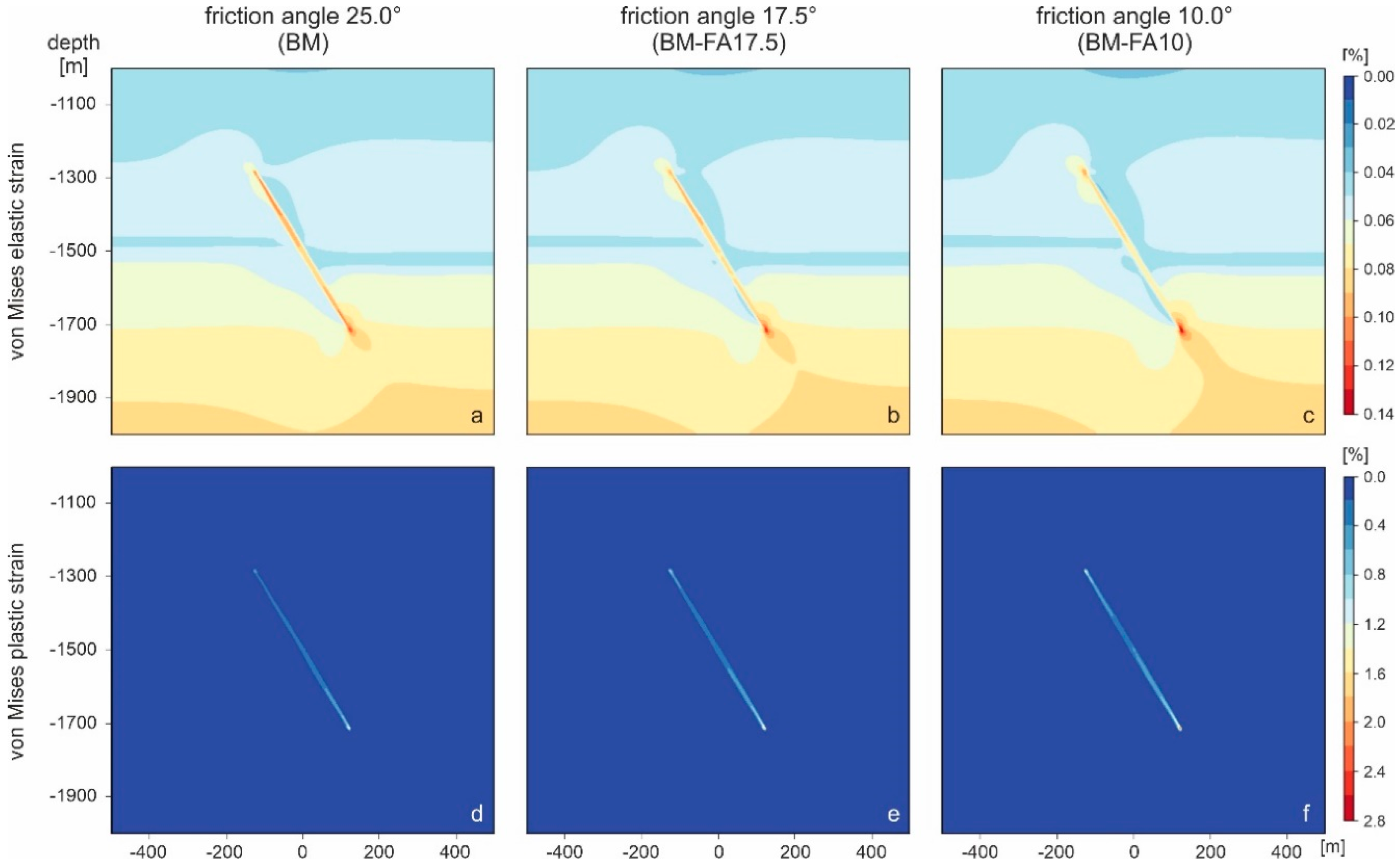
Figure 12.
Maximum values of the (a) magnitude of the effective maximum principal stress (S1,eff), and (b) the von Mises elastic strain for different Young’s moduli and Poisson’s ratios assigned to the fault zone. (c) Comparison of von Mises elastic, plastic and total strain after five years of injection for different Young’s moduli and a Poisson’s ratio of 0.25.

Figure 13.
Maximum values of the (a) magnitude of the effective maximum principal stress (S1,eff) and (b) the von Mises plastic strain after five years of injection for different cohesion values and friction angles assigned to the fault zone.
Figure 13.
Maximum values of the (a) magnitude of the effective maximum principal stress (S1,eff) and (b) the von Mises plastic strain after five years of injection for different cohesion values and friction angles assigned to the fault zone.
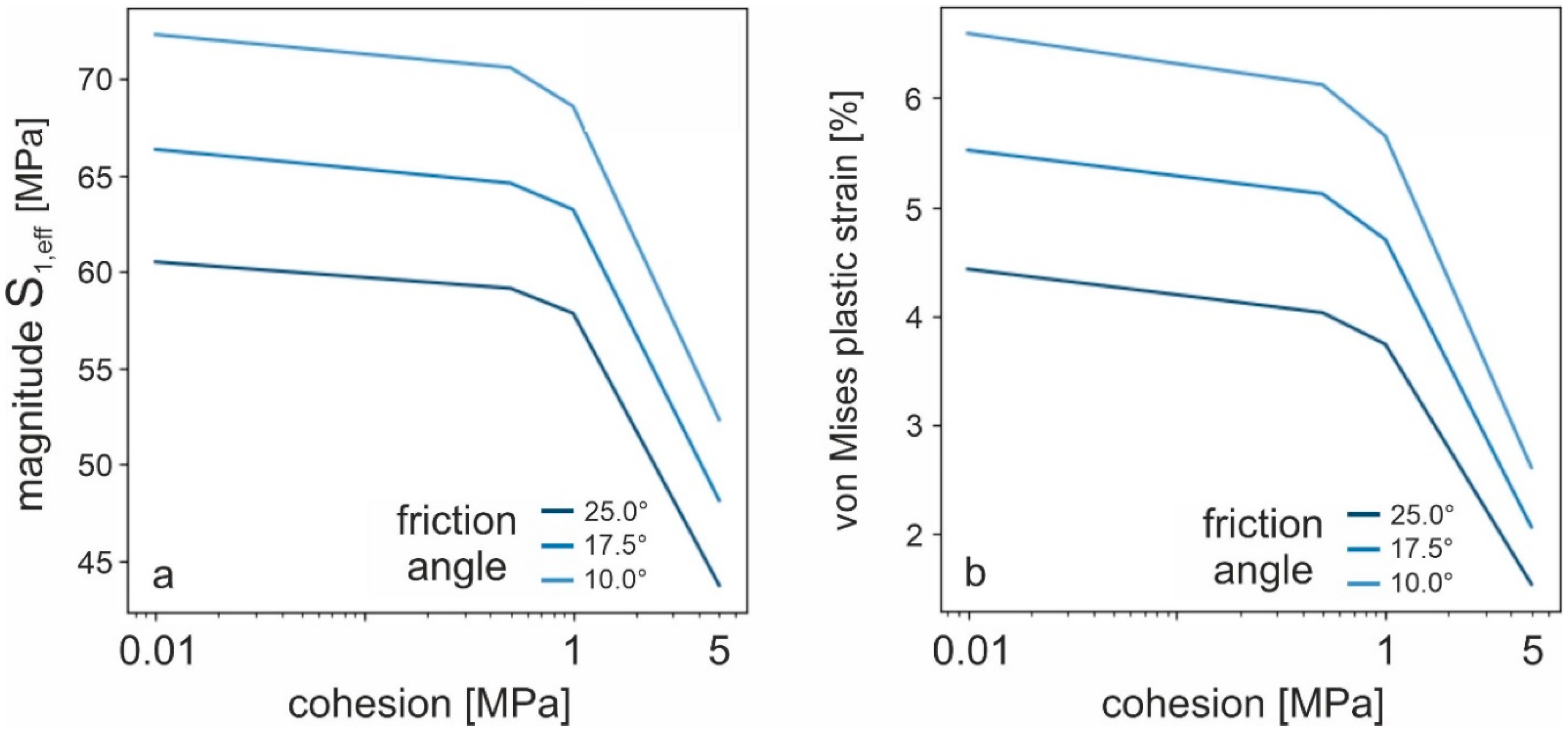
Figure 14.
Spatial variation in the magnitude of the effective maximum principal stress (S1,eff) after five years of injection for three different cohesion values and three different friction angles assigned to the fault zone rocks. The cohesion is varied from top to bottom row (a,d,g;b,e,h;c,f,i) and the friction angle is varied from left to right (a–c,d–f,g–i).
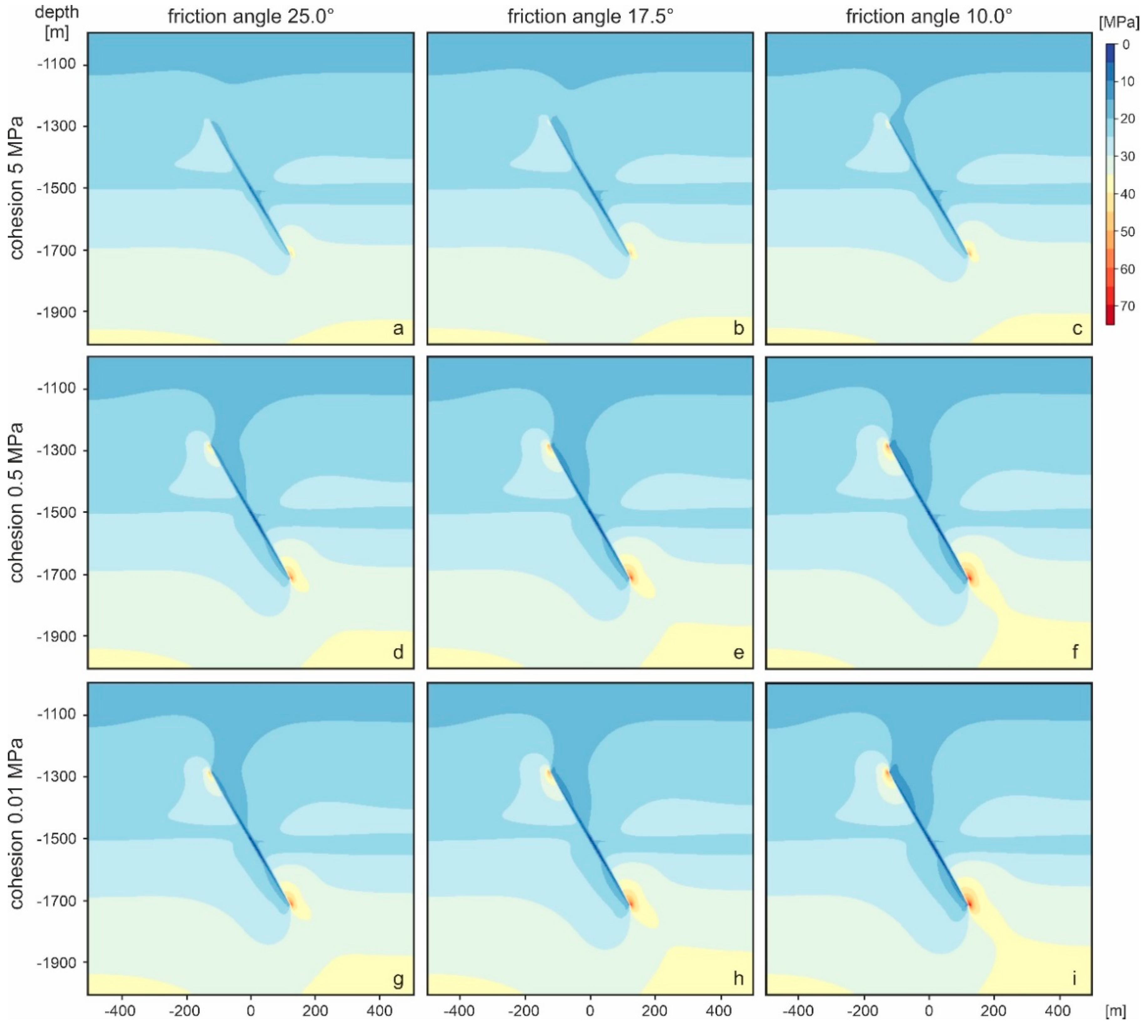

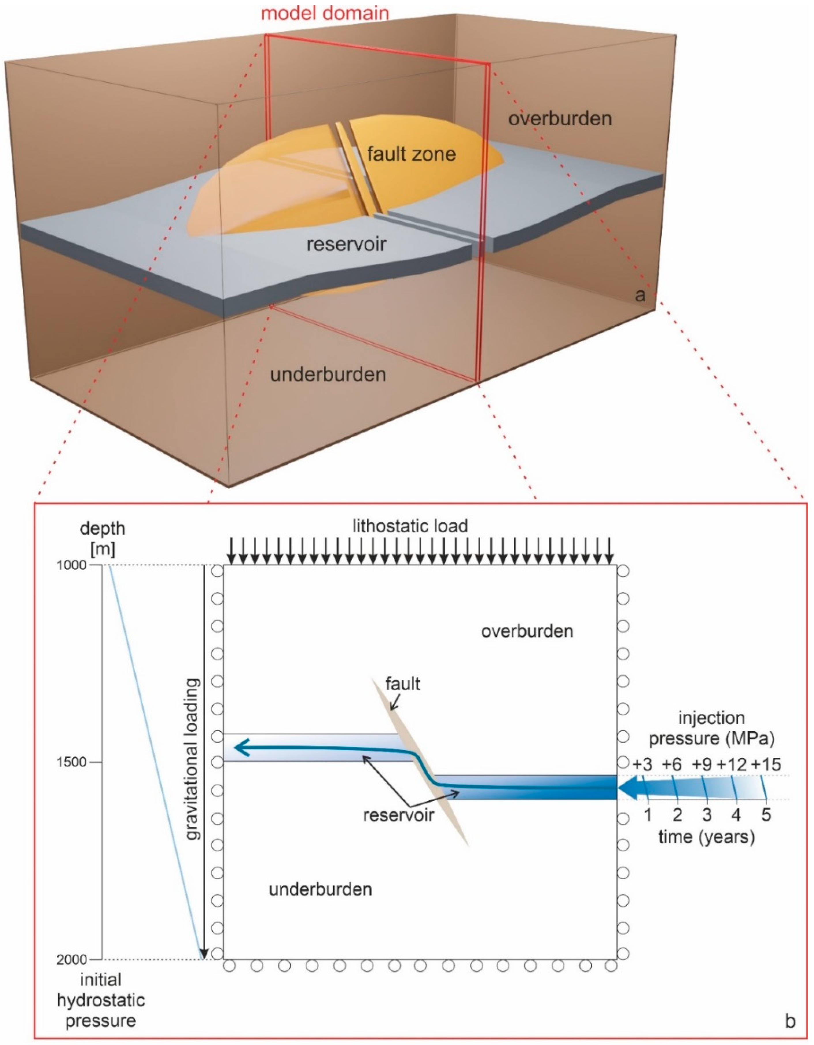
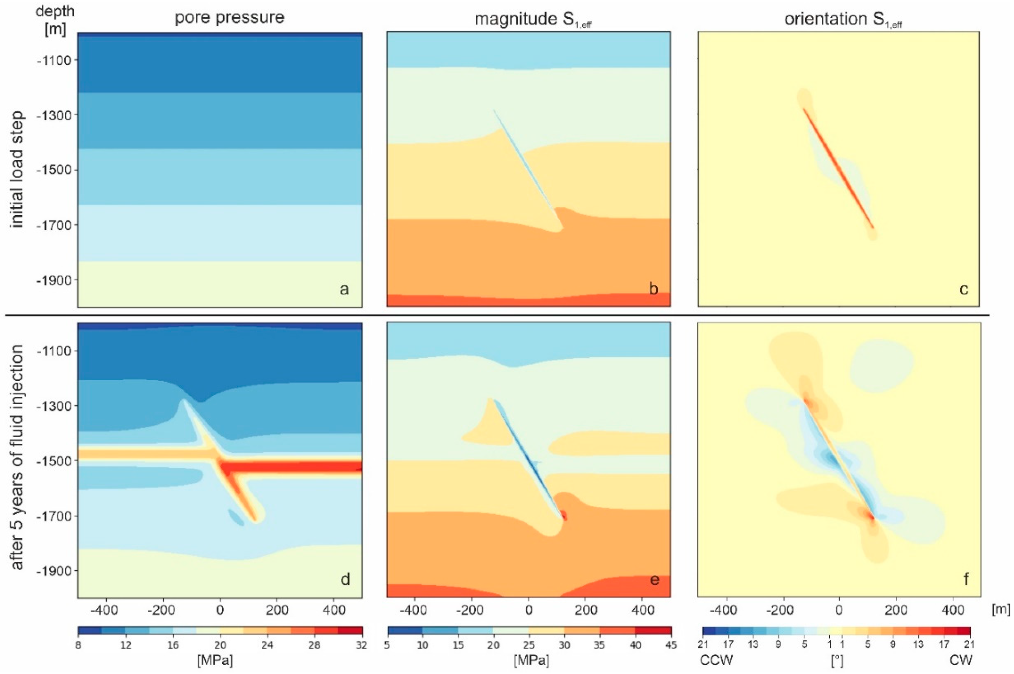
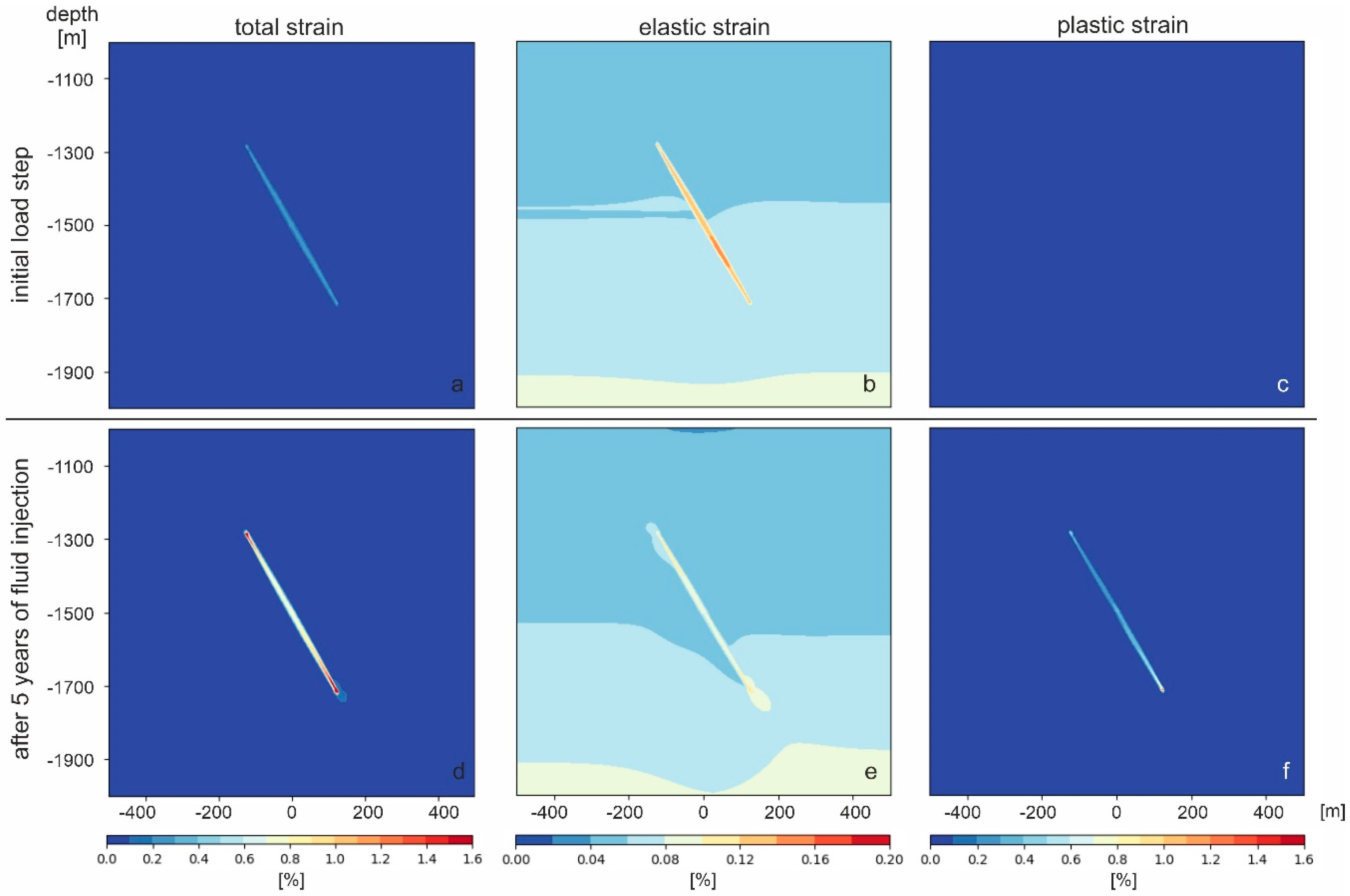
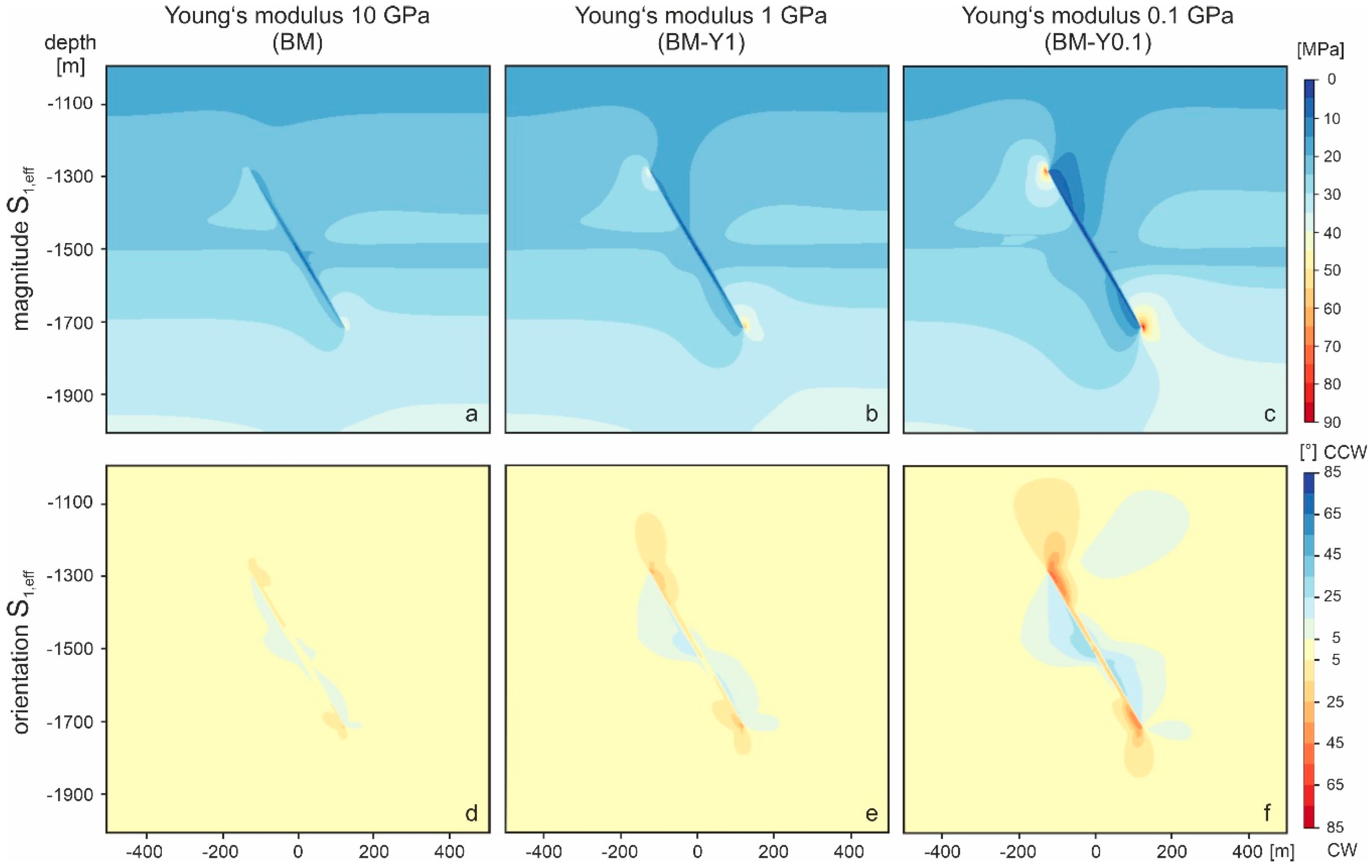
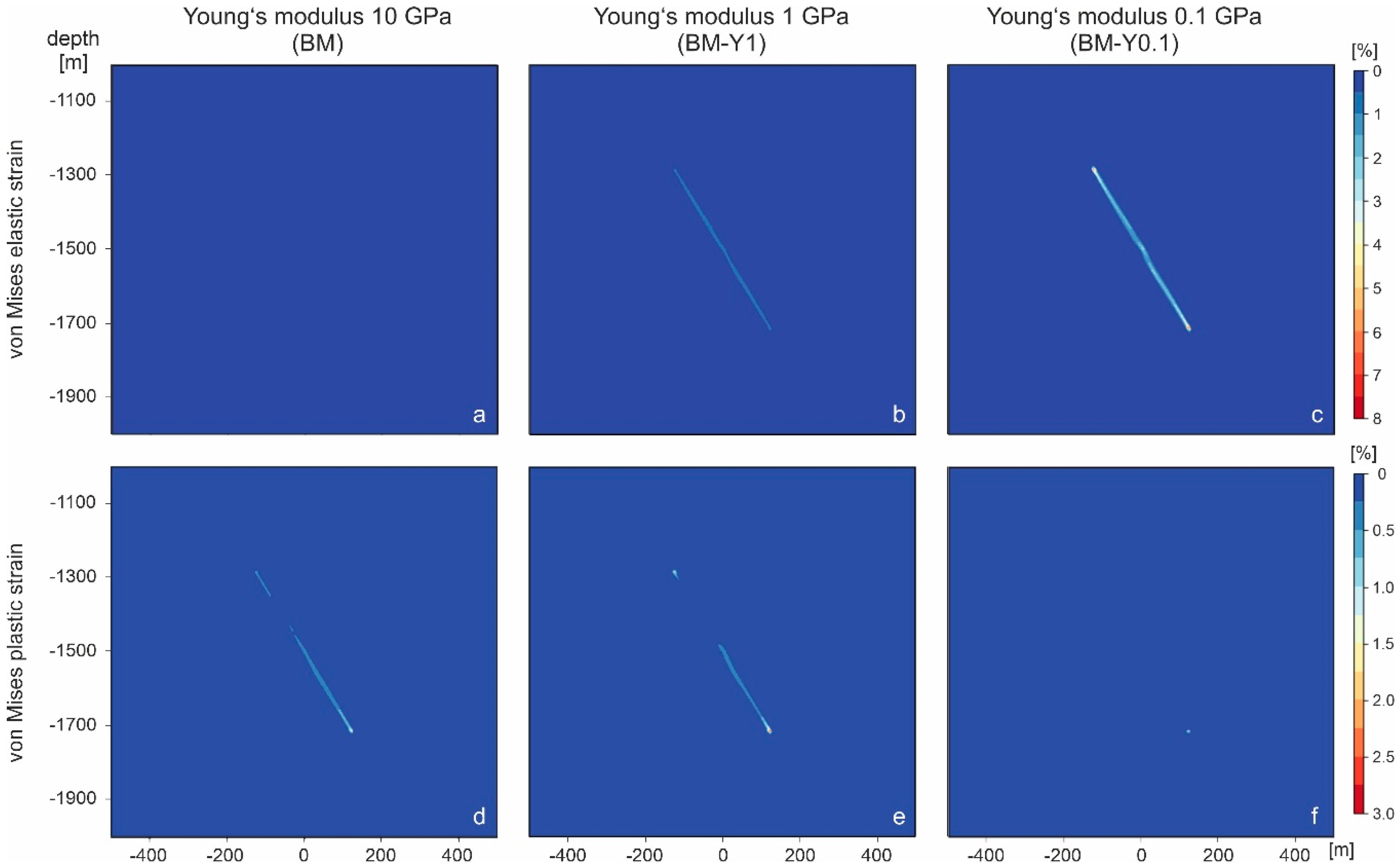
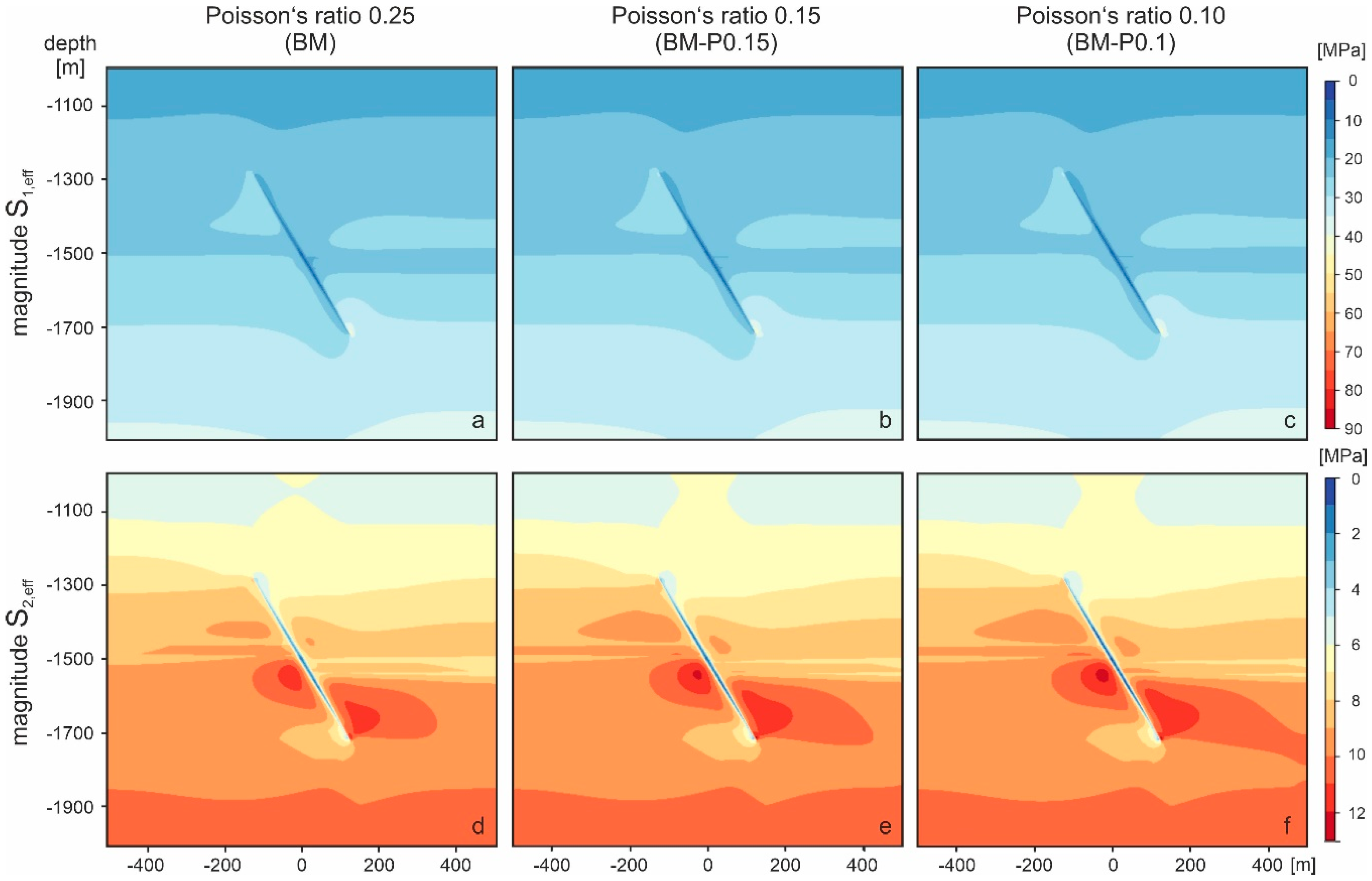
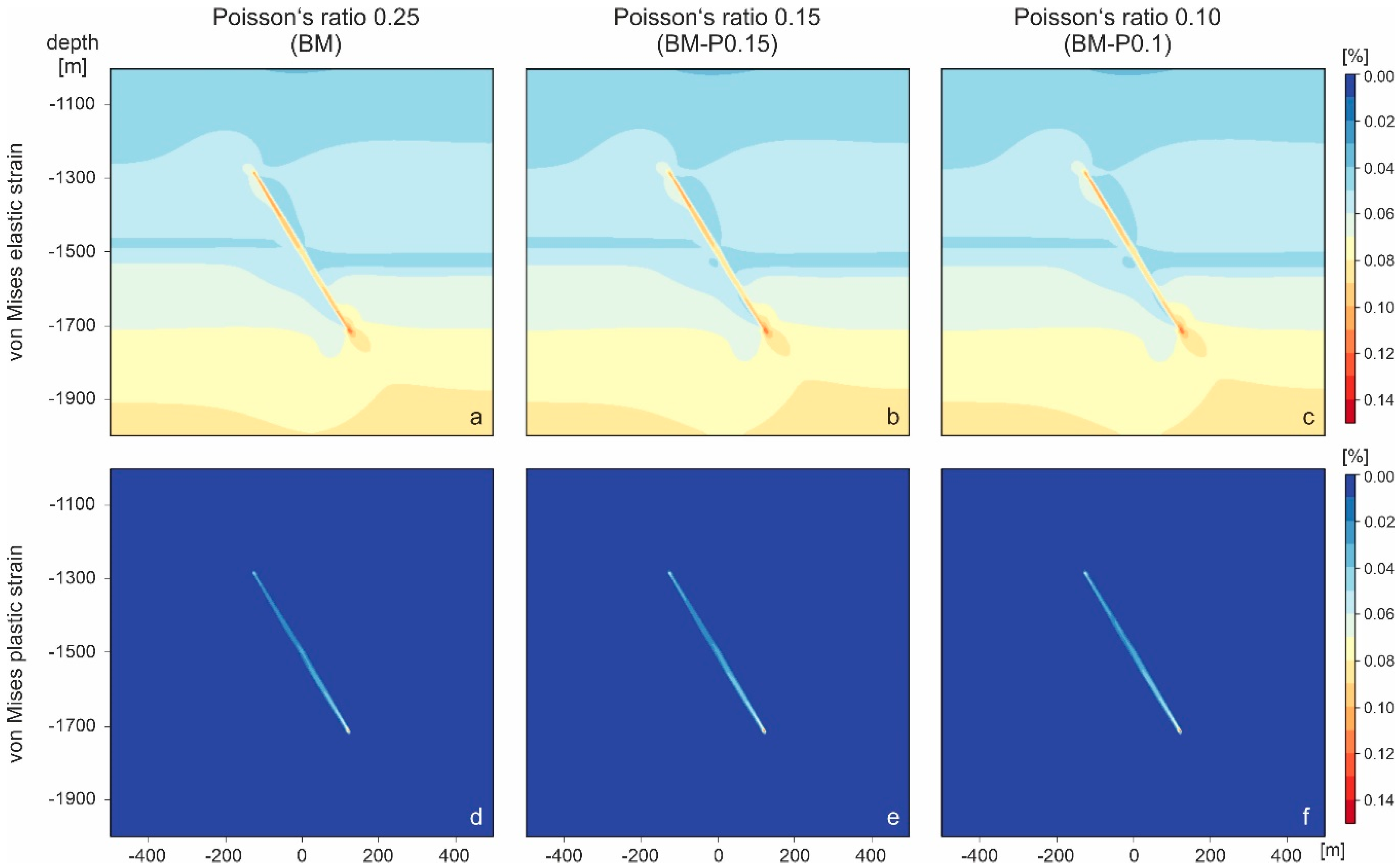
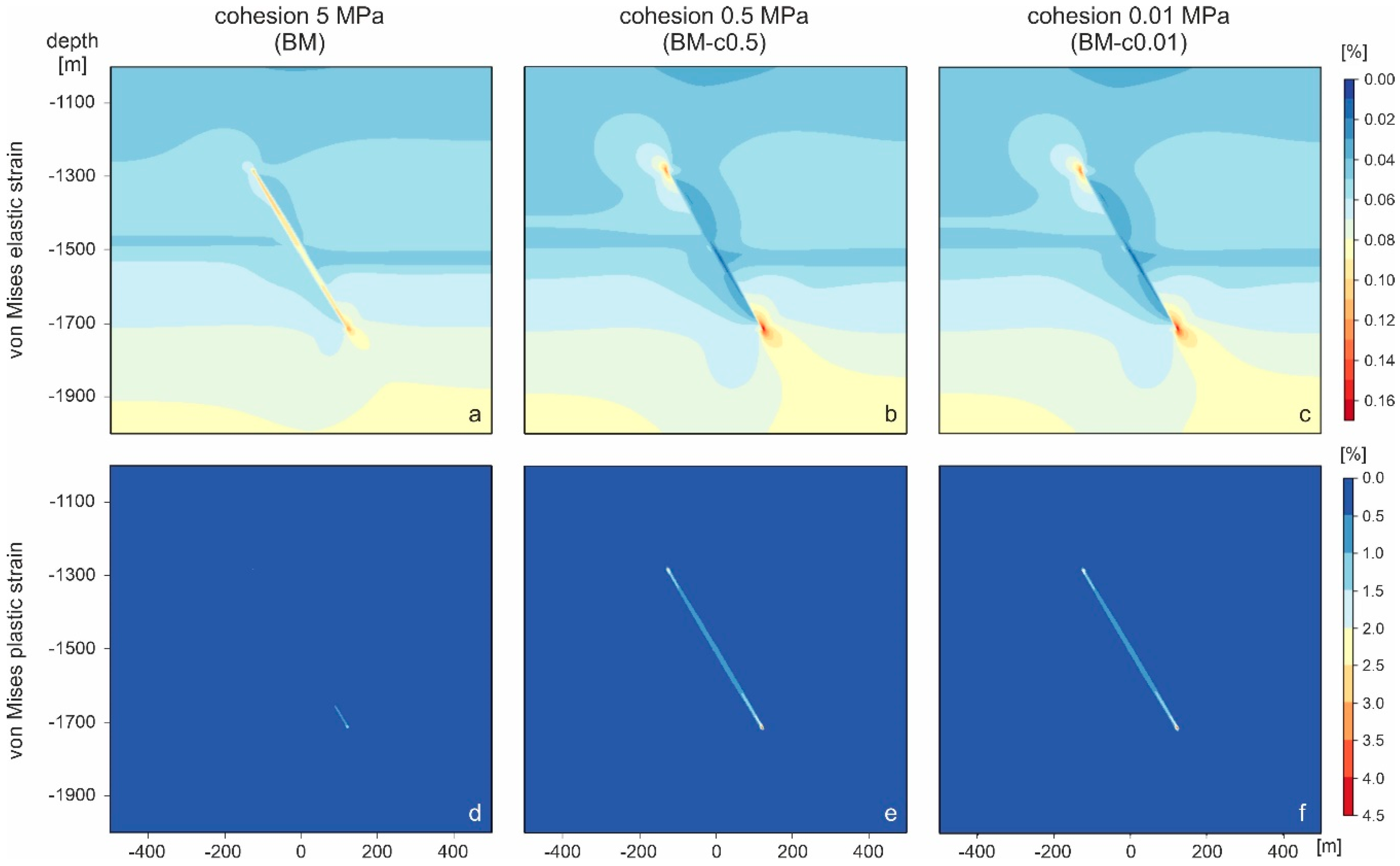
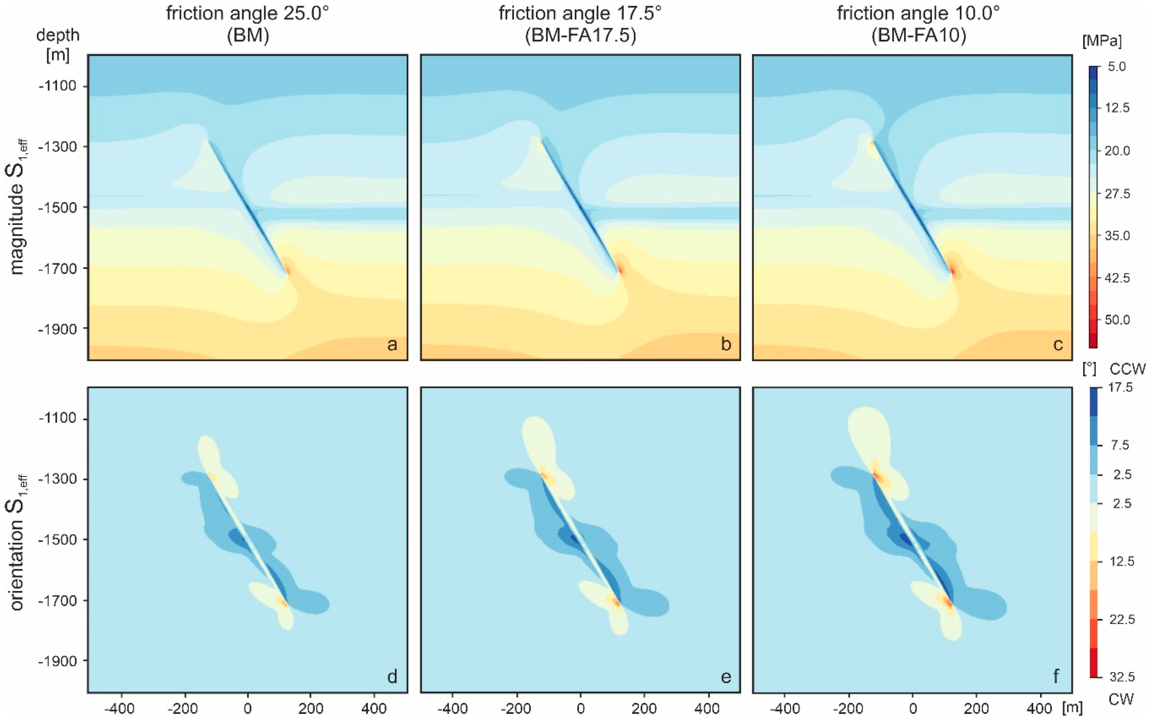
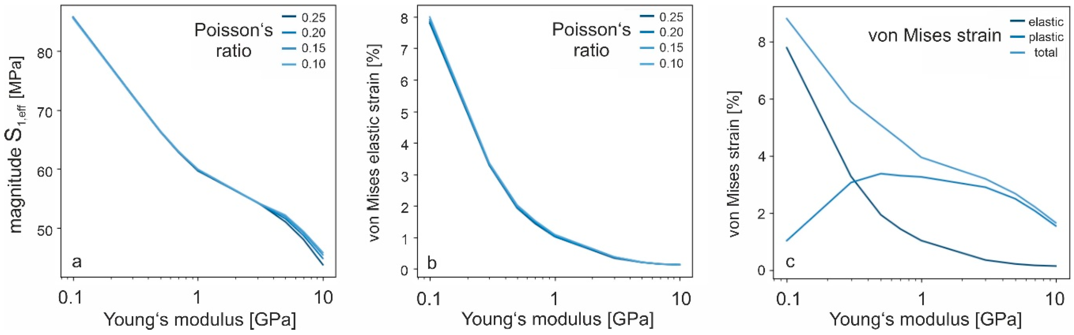
Table 1.
Hydraulic and mechanical parameters used for the three model units.
| Mechanical | Symbol | Fault Zone | Reservoir | Over-/Underburden |
|---|---|---|---|---|
| Young’s modulus (GPa) | E | 0.1–10 | 30 | 30 |
| Poissons’ ratio (-) | v | 0.1–0.25 | 0.23 | 0.23 |
| Friction angle (°) | φ | 10–25 | 40 | 40 |
| Cohesion (MPa) | c | 0.01–5 | 20 | 20 |
| Tensile strength (MPa) | T0 | 5 | 20 | 20 |
| Density (kg/m3) | ρ | 2400 | 2400 | 2400 |
| Hydraulic | ||||
| Biot coefficient (-) | α | 0.9 | 0.5 | 0.5 |
| Permeability (m2) | k | 10−14 | 5−12 | 10−17 |
Table 2.
Overview of the 87 scenarios studied and the corresponding model names. The scenarios differ regarding the elastic and the frictional properties assigned to the model unit representing the fault zone.
Table 2.
Overview of the 87 scenarios studied and the corresponding model names. The scenarios differ regarding the elastic and the frictional properties assigned to the model unit representing the fault zone.
| Model Name | Young’s Modulus (GPa) | Poisson’s Ratio (-) | Cohesion (MPa) | Friction Angle (°) |
|---|---|---|---|---|
| BM | 10 | 0.25 | 5 | 25.0 |
| BM-P0.20 | 10 | 0.20 | 5 | 25.0 |
| BM-P0.15 | 10 | 0.15 | 5 | 25.0 |
| BM-P0.10 | 10 | 0.10 | 5 | 25.0 |
| BM-FA17.5 | 10 | 0.25 | 5 | 17.5 |
| BM-FA10.0 | 10 | 0.25 | 5 | 10.0 |
| BM-c1 | 10 | 0.25 | 1 | 25.0 |
| BM-c1-FA17.5 | 10 | 0.25 | 1 | 17.5 |
| BM-c1-FA10.0 | 10 | 0.25 | 1 | 10.0 |
| BM-c0.5 | 10 | 0.25 | 0.5 | 25.0 |
| BM-c0.5-FA17.5 | 10 | 0.25 | 0.5 | 17.5 |
| BM-c0.5-FA10.0 | 10 | 0.25 | 0.5 | 10.0 |
| BM-c0.1 | 10 | 0.25 | 0.1 | 25.0 |
| BM-c0.1-FA17.5 | 10 | 0.25 | 0.1 | 17.5 |
| BM-c0.1-FA10.0 | 10 | 0.25 | 0.1 | 10.0 |
| BM-c0.05 | 10 | 0.25 | 0.05 | 25.0 |
| BM-c0.05-FA17.5 | 10 | 0.25 | 0.05 | 17.5 |
| BM-c0.05-FA10.0 | 10 | 0.25 | 0.05 | 10.0 |
| BM-c0.01 | 10 | 0.25 | 0.01 | 25.0 |
| BM-c0.01-FA17.5 | 10 | 0.25 | 0.01 | 17.5 |
| BM-c0.01-FA10.0 | 10 | 0.25 | 0.01 | 10.0 |
| BM-Y7 | 7 | 0.25 | 5 | 25.0 |
| BM-Y7-P0.20 | 7 | 0.25 | 5 | 25.0 |
| BM-Y7-P0.15 | 7 | 0.25 | 5 | 25.0 |
| BM-Y7-P0.10 | 7 | 0.25 | 5 | 25.0 |
| BM-Y5 | 5 | 0.25 | 5 | 25.0 |
| BM-Y5-P0.20 | 5 | 0.25 | 5 | 25.0 |
| BM-Y5-P0.15 | 5 | 0.25 | 5 | 25.0 |
| BM-Y5-P0.10 | 5 | 0.25 | 5 | 25.0 |
| BM-Y3 | 3 | 0.25 | 5 | 25.0 |
| BM-Y3-P0.20 | 3 | 0.25 | 5 | 25.0 |
| BM-Y3-P0.15 | 3 | 0.25 | 5 | 25.0 |
| BM-Y3-P0.10 | 3 | 0.25 | 5 | 25.0 |
| BM-Y1 | 1 | 0.25 | 5 | 25.0 |
| BM-Y1-P0.20 | 1 | 0.20 | 5 | 25.0 |
| BM-Y1-P0.15 | 1 | 0.15 | 5 | 25.0 |
| BM-Y1-P0.10 | 1 | 0.10 | 5 | 25.0 |
| BM-Y1-FA17.5 | 1 | 0.25 | 5 | 17.5 |
| BM-Y1-FA10.0 | 1 | 0.25 | 5 | 10.0 |
| BM-Y1-c1 | 1 | 0.25 | 1 | 25.0 |
| BM-Y1-c1-FA17.5 | 1 | 0.25 | 1 | 17.5 |
| BM-Y1-c1-FA10.0 | 1 | 0.25 | 1 | 10.0 |
| BM-Y1-c0.5 | 1 | 0.25 | 0.5 | 25.0 |
| BM-Y1-c0.5-FA17.5 | 1 | 0.25 | 0.5 | 17.5 |
| BM-Y1-c0.5-FA10.0 | 1 | 0.25 | 0.5 | 10.0 |
| BM-Y1-c0.1 | 1 | 0.25 | 0.1 | 25.0 |
| BM-Y1-c0.1-FA17.5 | 1 | 0.25 | 0.1 | 17.5 |
| BM-Y1-c0.1-FA10.0 | 1 | 0.25 | 0.1 | 10.0 |
| BM-Y1-c0.05 | 1 | 0.25 | 0.05 | 25.0 |
| BM-Y1-c0.05-FA17.5 | 1 | 0.25 | 0.05 | 17.5 |
| BM-Y1-c0.05-FA10.0 | 1 | 0.25 | 0.05 | 10.0 |
| BM-Y1-c0.01 | 1 | 0.25 | 0.01 | 25.0 |
| BM-Y1-c0.01-FA17.5 | 1 | 0.25 | 0.01 | 17.5 |
| BM-Y1-c0.01-FA10.0 | 1 | 0.25 | 0.01 | 10.0 |
| BM-Y0.7 | 0.7 | 0.25 | 5 | 25.0 |
| BM-Y0.7-P0.20 | 0.7 | 0.25 | 5 | 25.0 |
| BM-Y0.7-P0.15 | 0.7 | 0.25 | 5 | 25.0 |
| BM-Y0.7-P0.10 | 0.7 | 0.25 | 5 | 25.0 |
| BM-Y0.5 | 0.5 | 0.25 | 5 | 25.0 |
| BM-Y0.5-P0.20 | 0.5 | 0.25 | 5 | 25.0 |
| BM-Y0.5-P015 | 0.5 | 0.25 | 5 | 25.0 |
| BM-Y0.5-P0.10 | 0.5 | 0.25 | 5 | 25.0 |
| BM-Y0.3 | 0.3 | 0.25 | 5 | 25.0 |
| BM-Y0.3-P0.20 | 0.3 | 0.25 | 5 | 25.0 |
| BM-Y0.3-P0.15 | 0.3 | 0.25 | 5 | 25.0 |
| BM-Y0.3-P0.10 | 0.3 | 0.25 | 5 | 25.0 |
| BM-Y0.1 | 0.1 | 0.25 | 5 | 25.0 |
| BM-Y0.1-P0.20 | 0.1 | 0.20 | 5 | 25.0 |
| BM-Y0.1-P0.15 | 0.1 | 0.15 | 5 | 25.0 |
| BM-Y0.1-P0.10 | 0.1 | 0.10 | 5 | 25.0 |
| BM-Y0.1-FA17.5 | 0.1 | 0.25 | 5 | 17.5 |
| BM-Y0.1-FA10.0 | 0.1 | 0.25 | 5 | 10.0 |
| BM-Y0.1-c1 | 0.1 | 0.25 | 1 | 25.0 |
| BM-Y0.1-c1-FA17.5 | 0.1 | 0.25 | 1 | 17.5 |
| BM-Y0.1-c1-FA10.0 | 0.1 | 0.25 | 1 | 10.0 |
| BM-Y0.1-c0.5 | 0.1 | 0.25 | 0.5 | 25.0 |
| BM-Y0.1-c0.5-FA17.5 | 0.1 | 0.25 | 0.5 | 17.5 |
| BM-Y0.1-c0.5-FA10.0 | 0.1 | 0.25 | 0.5 | 10.0 |
| BM-Y0.1-c0.1 | 0.1 | 0.25 | 0.1 | 25.0 |
| BM-Y0.1-c0.1-FA17.5 | 0.1 | 0.25 | 0.1 | 17.5 |
| BM-Y0.1-c0.1-FA10.0 | 0.1 | 0.25 | 0.1 | 10.0 |
| BM-Y0.1-c0.05 | 0.1 | 0.25 | 0.05 | 25.0 |
| BM-Y0.1-c0.05-FA17.5 | 0.1 | 0.25 | 0.05 | 17.5 |
| BM-Y0.1-c0.05-FA10.0 | 0.1 | 0.25 | 0.05 | 10.0 |
| BM-Y0.1-c0.01 | 0.1 | 0.25 | 0.01 | 25.0 |
| BM-Y0.1-c0.01-FA17.5 | 0.1 | 0.25 | 0.01 | 17.5 |
| BM-Y0.1-c0.01-FA10.0 | 0.1 | 0.25 | 0.01 | 10.0 |
© 2020 by the authors. Licensee MDPI, Basel, Switzerland. This article is an open access article distributed under the terms and conditions of the Creative Commons Attribution (CC BY) license (http://creativecommons.org/licenses/by/4.0/).
Share and Cite
MDPI and ACS Style
Treffeisen, T.; Henk, A. Elastic and Frictional Properties of Fault Zones in Reservoir-Scale Hydro-Mechanical Models—A Sensitivity Study. Energies 2020, 13, 4606. https://doi.org/10.3390/en13184606
AMA Style
Treffeisen T, Henk A. Elastic and Frictional Properties of Fault Zones in Reservoir-Scale Hydro-Mechanical Models—A Sensitivity Study. Energies. 2020; 13(18):4606. https://doi.org/10.3390/en13184606
Chicago/Turabian StyleTreffeisen, Torben, and Andreas Henk. 2020. "Elastic and Frictional Properties of Fault Zones in Reservoir-Scale Hydro-Mechanical Models—A Sensitivity Study" Energies 13, no. 18: 4606. https://doi.org/10.3390/en13184606
Note that from the first issue of 2016, this journal uses article numbers instead of page numbers. See further details here.