Parameters Identification of Equivalent Model of Permanent Magnet Synchronous Generator (PMSG) Wind Farm Based on Analysis of Trajectory Sensitivity

Abstract

As wind farms have great influences on power system stability, it is essential to develop an adaptive as well as robust equivalent model of it. In this paper, a detailed equivalent model of PMSG wind farm and initialization method is developed. The trajectory sensitivity of parameters is analyzed. Then, the key parameters are estimated using improved Genetic Learning Particle Swarm Optimization (GLPSO) hybrid algorithm with phasor measurement unit (PMU). The description and generalization capability, stability for parameter identification of the equivalent model under wake effects, and when some wind turbines are off-line or wind speed is unknown after an event are analyzed. The maximum differences between the values of estimated parameters and their real ones are less than 10% for the proportional magnification constant of DC voltage controller $K_{\mathrm{p}2}$ and grid side current controller $K_{\mathrm{p}3}$. The convergence rate and global optimization performance of the improved GLPSO hybrid algorithm is 0.5 times higher than the classical particle swarm optimization algorithm (PSO) and genetic algorithm (GA).

1. Introduction

Connecting a large scale PMSG wind farm to grid brings about great influence on angle [1,2], voltage [3,4] and frequency [5,6] stability of power system. If detailed model of PMSG wind farm is built to simulate all wind turbines, the complexity and simulation time will greatly increase [7]. Therefore, the establishment of a simplified, accurate and effective wind farm equivalent model is essential for analysis and control of power system [8].

Wind farm can be equivalent to a single machine [9,10] or multi-machines [11,12]. The equivalent methods mainly include aggregation method using detailed physical parameters [13] or parameters estimation method using PMU data in the point of common interconnection. Yingchen Zhang et al. report that the output from the standard model cannot match the measurements of he DFIG wind farm [14]. J. Brochu et al. carry out short circuit test on field and show that for stability and electromagnetic transient studies, single machine representation of wind farm after disturbance provide good and adequate results [15]. Jin Lin et al. analyze the wide-area trajectory sensitivity for parameters of constant speed induction generator wind farm. GA is used to estimate the parameters [16]. Xueyang Cheng et al. estimate the key parameters of the equivalent model of DFIG wind farm using PSO gradient search optimization with PMU data [17]. Yinfeng Wang et al. use improved GA to strengthen the capability of global optimization [18]. L. P. Kunjumuhammed et al. pointed out that aggregation methods must be improved to enhance precision [19]. Dong-Eok Kim et al. formulate a linear model for DFIG wind farm. The recursive least square method is used to estimate the parameters [20]. Yuhao Zhou et al. propose an aggregation method of collecting system. The robustness of the equivalent model for DFIG wind farm when some wind turbines are offline is analyzed [21]. Jian Zhang et al. consider the control system limiting units of grid side (GSC) and machine side converters (MSC) of DFIG wind turbine in the parameters estimation process. As an outcome, the precision are greatly improved [22]. Xueping Pan et al. propose a simplified model of PMSG wind turbine, in which the mechanical subsystem is neglected. The combination of PSO method and Levenberg-Marquardt method is used to estimate the simplified model parameters. Furthermore, the simplified PMSG wind turbine model and the classical load model are paralleled to illustrate the generalized synthesis load in the distribution network [23]. However, the permanent magnet flux linkage of PMSG is not identified. Moreover, the parameters of PMSG wind farm are identified with load parameters. Peipeng Zhou et al. formulate the frequency-domain impedance equivalent model of PMSG wind farms to cope with sub-synchronization and sup-synchronization oscillation problems [24]. Parameter sensitivity of wind generator input admittance to wind speed is analyzed. The input admittance and the participation factor for the dominant oscillation mode are used as the indexes of dividing groups. Based on the circuit equations, node-by-node aggregation is proposed. However, this approach still belongs to the aggregation method. After long-time running, the dynamical characteristics may be changed due to the change of parameters of each PMSG wind turbine. As a result, this method cannot be applicable any longer.

At present, a large number of researches focus on DFIG wind farm. The literature on equivalent model of PMSG wind farm is very rare. In this paper, in view of the fact that the traditional aggregation method cannot solve the problem of parameter variation during long-time running of wind farms, and manufacturers regard control system parameters as commercial secrets, we propose that the time-varying and control parameters with high sensitivity are identified using improved GLPSO hybrid algorithm while the values of other parameters are fixed to aggregated or typical values.

The organization of this paper is as follows. In Section 2, the initialization method of the equivalent model of a PMSG wind farm is proposed. In Section 3, the trajectory sensitivity analysis of time-varying and control system parameters is performed. In Section 4, parameters identification method is formulated. In Section 5, simulation cases are conducted. Conclusions are summarized in Section 6.

2. Initialization Method for the Equivalent Model of PMSG Wind Turbine

Suppose the steady state voltage magnitude, injected active and reactive power of common interconnection point of wind farm is denoted by $V_0$, $P_0$ and $Q_0$. Then current magnitude squared injecting into the grid from wind farm is given by:

$$I_0^2=\frac{P_0^2+Q_0^2}{V_0^2}$$

(1)

The active power loss on the coupling and filter inductor is given by:

$$P_{\mathrm{loss}1}=I_0^2{R}_{\mathrm{g}}$$

(2)

where $R_{\mathrm{g}}$ is the resistance of coupling and filter inductor. The stator loss of PMSG is:

$$P_{\mathrm{loss}2}=i_{\mathrm{qs}}^2{R}_{\mathrm{s}}$$

(3)

where $R_{\mathrm{s}}$ is the PMSG stator resistance. $i_{\mathrm{qs}}$ is the q-axis current of stator of PMSG.

The electromagnetic power of PMSG is:

$$P_{\mathrm{EM}}=-E{i}_{\mathrm{qs}}=-{\omega }_{\mathrm{e}}{\psi }_{\mathrm{PM}}{i}_{\mathrm{qs}}$$

(4)

where $E$ is the electromotive force of PMSG. ${\omega }_{\mathrm{e}}$ is the electrical angular velocity of rotor. ${\psi }_{\mathrm{PM}}$ is permanent magnet flux linkage of PMSG.

$P_{\mathrm{EM}}$ can be rewritten as:

$$P_{\mathrm{EM}}=P_0+P_{\mathrm{loss}1}+P_{\mathrm{loss}2}$$

(5)

Equations (3) and (4) are substituted into (5). Then Equation (6) can be obtained:

$$R_{\mathrm{s}}{i}_{\mathrm{qs}}^2+{\omega }_{\mathrm{e}}{\psi }_{\mathrm{PM}}{i}_{\mathrm{qs}}+P_{\mathrm{loss}1}+P_0=0$$

(6)

Generally, the optimal torque control is adopted. The reference of electro-magnetic torque is generally set as:

$$T_{\mathrm{opt}}=-k_{\mathrm{opt}}{\omega }_{\mathrm{e}}^2$$

(7)

where $k_{\mathrm{opt}}$ is the optimal torque-speed coefficient, which can be obtained according to the power-speed curve of PMSG wind turbine.

The electromagnetic torque of PMSG is given by:

$$T_{\mathrm{e}}={\psi }_{\mathrm{PM}}{i}_{\mathrm{qs}}$$

(8)

In steady state, the electromagnetic torque is equal to that of the control command. That is:

$$T_{\mathrm{opt}}=T_{\mathrm{e}}$$

(9)

Substituting (7) and (8) into (9), results in:

$$i_{\mathrm{qs}}=-\frac{k_{\mathrm{opt}}{\omega }_{\mathrm{e}}^2}{{\psi }_{\mathrm{PM}}}$$

(10)

Equation (10) is substituted into (6). Then Equation (11) can be obtained:

$$R_{\mathrm{s}}{\left(\frac{k_{\mathrm{opt}}}{{\psi }_{\mathrm{PM}}}\right)}^2{\omega }_{\mathrm{e}}^4-k_{\mathrm{opt}}{\omega }_{\mathrm{e}}^3+P_0+P_{\mathrm{loss}1}=0$$

(11)

When solving (11), resistance $R_s$ can be neglected first. Thus, (12) can be obtained. Then, according to (13), the estimation of steady state rotational electric angular speed of rotor ${\omega }_{e0}$ can be obtained. Taking ${\omega }_{e0}$ as the initial value, the Newton-Raphson approach is adopted to compute the rotational electric angular speed of rotor by solving Equation (11).

$$-k_{\mathrm{opt}}{\omega }_{\mathrm{e}}^3+P_0+P_{\mathrm{loss}1}=0$$

(12)

$${\omega }_{\mathrm{e}0}=\sqrt[3]{\frac{P_0+P_{\mathrm{loss}1}}{k_{\mathrm{opt}}}}$$

(13)

3. Control System and Time-Varying Parameters Trajectory Sensitivity

3.1. The Necessity of Trajectory Sensitivity Analysis

In the equivalent model, there are many parameters. If all parameters are identified, it will inevitably consume a lot of computational time, and the identification results will be very dispersive. As a consequence, the equivalent model is very difficult to apply. Therefore, only the key parameters that have strong impact on power system dynamics need to be identified. As direct current (DC) capacitors, filter inductors and equivalent distribution network impedance are static components, they can be fixed to nameplate or technical manuals values, and are not identified. The specific aggregation methods can be found in [18]. Moreover, PMSG is a rotating element. After long-term operation, its stator resistance, reactance and flux linkage may differ enormously from nameplate data and should be taken as candidate parameters to be identified. Although the inertial time constant is less time-varying, its value is usually not listed in the nameplate and technical manual. Therefore, it is taken as a candidate parameter to be identified as well. Controller parameters are generally regarded as commercial secrets by manufacturers. Their values cannot be found in nameplate and technical manuals. Therefore, controller parameters should also be taken as candidate parameters to be identified. However, low sensitivity parameters in candidate parameters to be identified are generally difficult to identify accurately and can be fixed to typical values. Therefore, sensitivity analysis of candidate identified parameters is carried out in this paper to discern the high sensitivity parameters.

The relationship between sensitivity analysis and parameter identification is that the former guides the latter. That is, sensitivity analysis tells which parameters should be identified. If all the candidate identification parameters are identified without sensitivity analysis, the convergence rate of the program will be very slow, and the identification results will be very dispersive.

3.2. Algorithm of Trajectory Sensitivity Analysis

The computing method of trajectory sensitivity and its average value in theory is shown in Appendix A. However, the trajectory sensitivity and its average value are very hard to compute analytically according to Equation (A1)–(A3) in Appendix A. However, the numerical solution can be obtained using simulation software. The algorithm is as follows.

(1)

Firstly, a simulation example is built to set the candidate identification parameters to the nameplate or technical manuals values. If they cannot be found on the nameplate and technical manual, they are set as the typical values.

(2)

Then, the power flow is computed. After that, the transient analysis and computation are conducted. As a result, $P_0(t)$ and $Q_0(t)$ are recorded.

(3)

Increase the value of $k^{th}$ candidate identification parameter by 5% based on the value set in Step (1). Repeat step (2) to get $P_k(t)$ and $Q_k(t)$.

(4)

The trajectory sensitivity of the $k^{th}$ candidate identification parameter are computed as

$$S_{\mathrm{p}}^k\left(t\right)=\frac{P_k(t)-P_0(t)}{5\%P_0(t)}$$

(14)

$$S_{\mathrm{q}}^k\left(t\right)=\frac{Q_k(t){-\mathrm{Q}}_0(t)}{5\%Q_0(t)}$$

(15)

(5)

The average trajectory sensitivities of the $k^{th}$ candidate identification parameter for active as well as reactive power are computed as

$${\overline{S}}_{\mathrm{p}}^k=\frac{1}{N}{\displaystyle \sum _{t=1}^N\left|S_{\mathrm{p}}^k\left(t\right)\right|}$$

(16)

$${\overline{S}}_{\mathrm{q}}^k=\frac{1}{N}{\displaystyle \sum _{t=1}^N\left|S_{\mathrm{q}}^k\left(t\right)\right|}$$

(17)

where $N$ is the number of sample data.

(6)

Repeat Steps (2)–(5) to compute the trajectory sensitivity and average trajectory sensitivity of all candidate identification parameters.

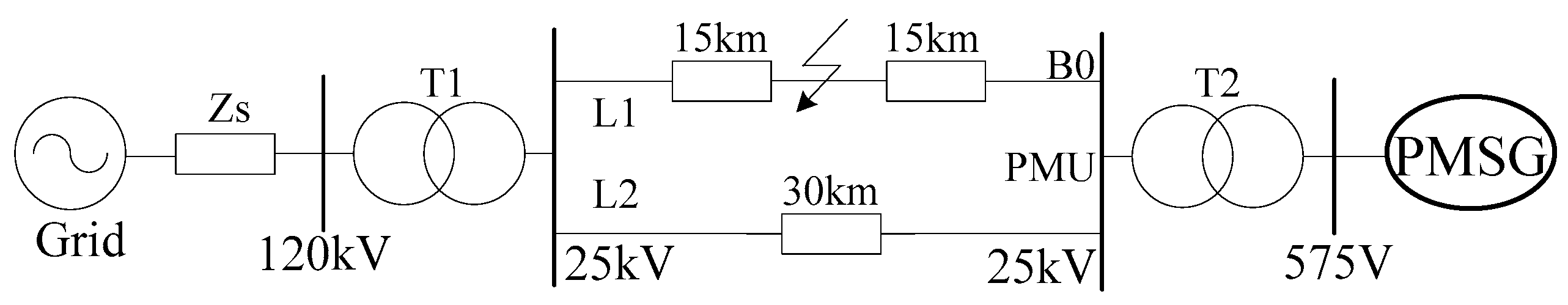
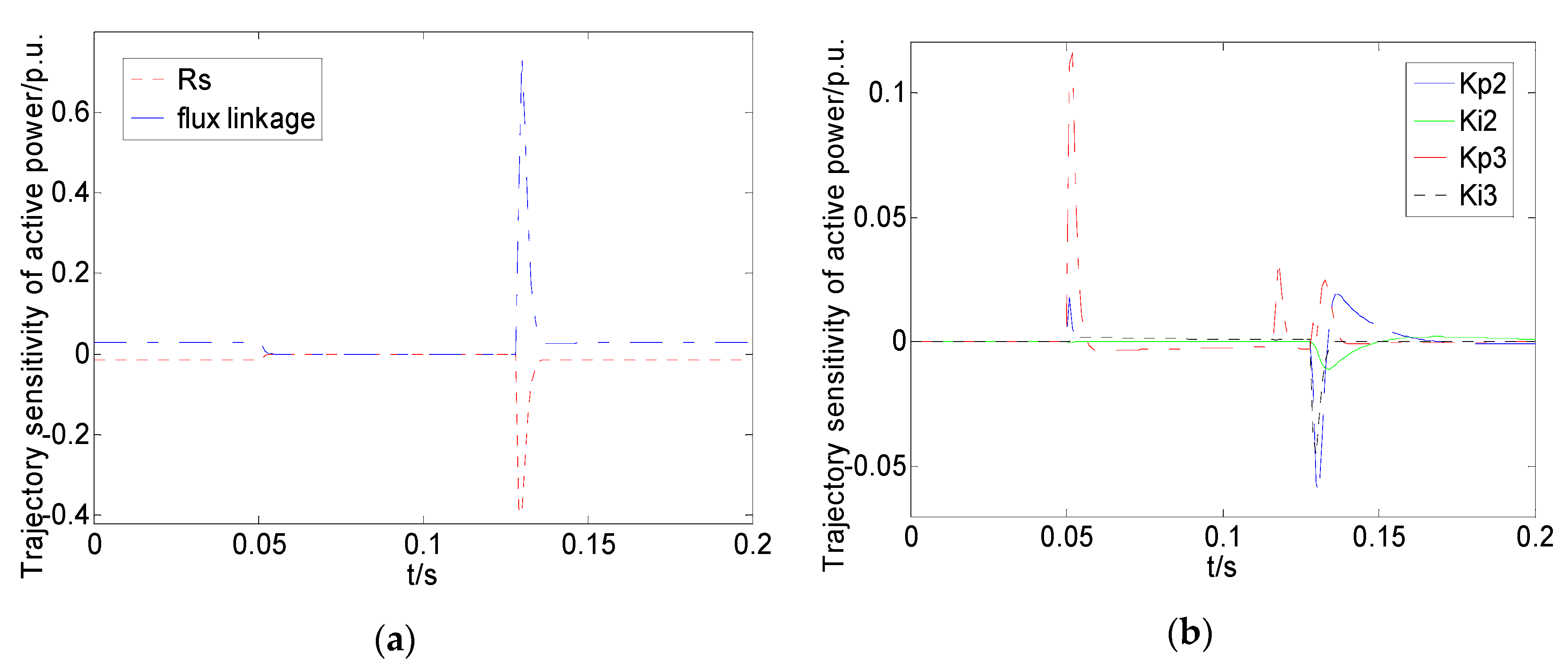
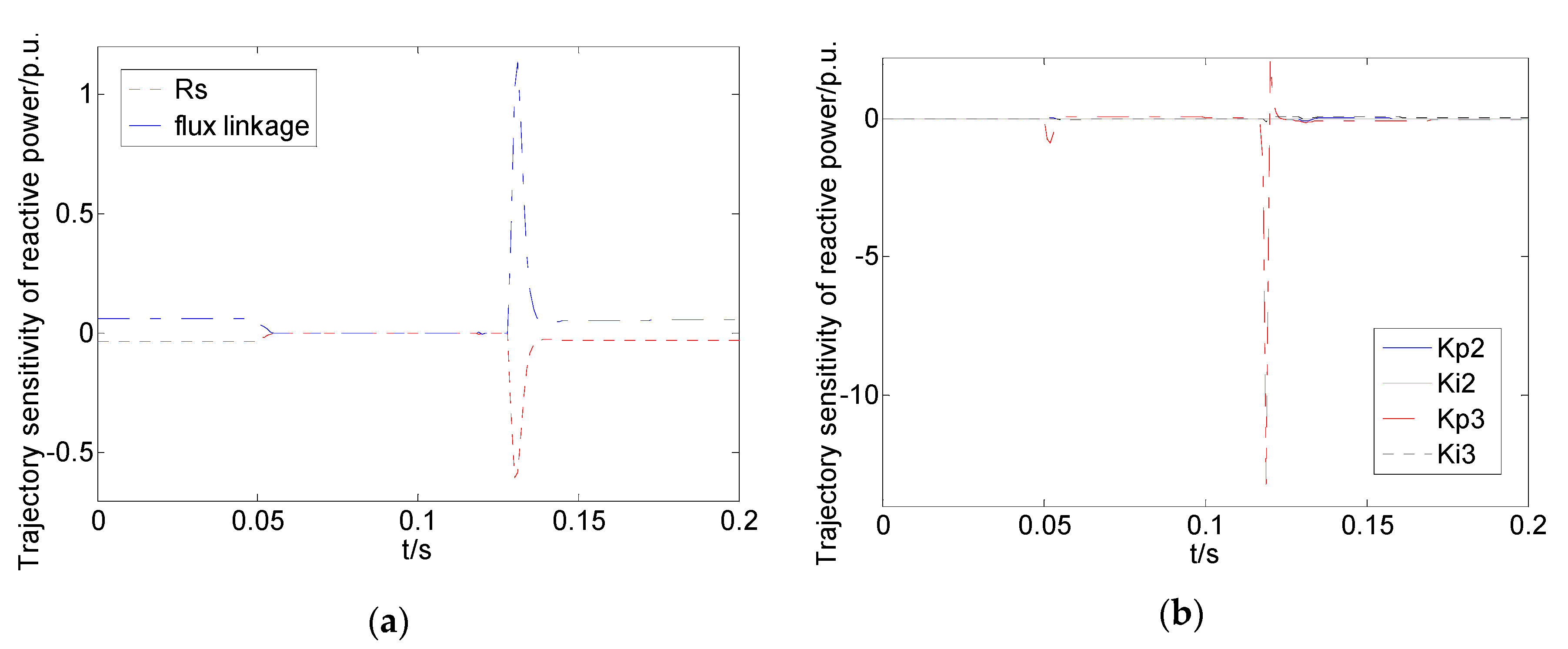
3.3. A Case of Trajectory Sensitivity Analysis

The trajectory sensitivity of the candidate identification parameters of the equivalent model is investigated using the simulation system shown in Figure 1. A round-rotor PMSG wind turbine with rated active power of 1.5 MW is connected to the 575 V bus. The parameters of physical and control system of the PMSG wind turbine are shown in

Table 1. Physical Parameters of 1.5-MW PMSG wind turbine.

Parameters	Values	Parameters	Values
Stator resistance (p.u.)	0.0272	Rated capacity of T2 (MVA)	2
Stator resistance (p.u.)	0.5131	T2 resistance (p.u.)	0.0015
Flux linkage (p.u.)	1.1884	Leakage reactance of T2 (p.u.)	0.0415
Inertial constant (s)	1.4393	Rated power factor of PMSG wind turbine	1.0
Rated capacity of MSC (p.u.)	1.0	Rated capacity of GSC (p.u.)	1.2
DC Bus Voltage (V)	1150	Filter resistance (p.u.)	0.03
DC capacitor (F)	0.01	Filter resistance (p.u.)	0.3

and

Table 2. Controller parameters of 1.5-MW PMSG wind turbine.

Parameters	Values	Parameters	Values
MSC current controller $K_{\mathrm{p}1}\left(\mathrm{p}.\mathrm{u}.\right)$	0.1361	GSC lower limit of reference current (p.u.)	−1.2
MSC current controller $K_{\mathrm{i}1}\left(\mathrm{p}.\mathrm{u}.\right)$	2.7221	Upper limit reference torque (p.u.)	1.1
DC voltage controller $K_{\mathrm{p}2}\left(\mathrm{p}.\mathrm{u}.\right)$	8	Lower limit reference torque (p.u.)	−1.1
DC current controller $K_{\mathrm{i}2}\left(\mathrm{p}.\mathrm{u}.\right)$	400	Pitch angle controller $K_{\mathrm{p}}\left(\mathrm{p}.\mathrm{u}.\right)$	200
GSC current controller $K_{\mathrm{p}3}\left(\mathrm{p}.\mathrm{u}.\right)$	0.83	Maximum pitch angle (°)	27
GSC current controller $K_{\mathrm{i}3}\left(\mathrm{p}.\mathrm{u}.\right)$	5	Maximum pitch angle change rate (°/s)	10
GSC upper limit of current (p.u.)	1.2	Minimal pitch angle change rate (°/s)	−10

, respectively. Doctor Jiayang Ruan, who is the author of many published papers on wind power generation, developed the detailed PMSG wind turbine model according to Ref. [25] which can be downloaded from Ref. [26]. We modify it to the phasor model using MATLAB/SIMULINK.

A three-phase short circuit fault with 8 and 1 ohms transition resistance, 4 cycles duration are respectively set to the midpoint of line L1. The simulation time lasts for 0.2 s. The voltage magnitude of bus B0 dips about 30% when the transition resistance is set to 8 ohm and 80% when the transition resistance is set to 1 ohm. The candidate identification parameters are increased by 5% in turn according to the values in Table 1 and Table 2.

The average trajectory sensitivity of each candidate identification parameter for 8-ohm transition resistance is shown in

Table 3. Average trajectory sensitivity of parameters when voltage dips about 30%.

Parameters	Active Power	Reactive Power	Parameters	Active Power	Reactive Power
$R_{\mathrm{s}}$	0.0157	0.0302	$K_{\mathrm{i}1}$	0.0000	0.0000
$L_{\mathrm{d}}$$L_{\mathrm{q}}$	0.0000	0.0000	$K_{\mathrm{p}2}$	0.0024	0.0045
$T_{\mathrm{j}}$	0.0000	0.0000	$K_{\mathrm{i}2}$	0.0009	0.0018
${\psi }_{\mathrm{PM}}$	0.0286	0.0560	$K_{\mathrm{p}3}$	0.0035	0.1444
$K_{\mathrm{p}1}$	0.0000	0.0000	$K_{\mathrm{i}3}$	0.0012	0.0239

. Clearly, the average trajectory sensitivity of stator reactance $L_{\mathrm{d}}$, $L_{\mathrm{q}}$, inertia time constant $T_{\mathrm{j}}$, proportional and integral magnifications of MSC control loop $K_{\mathrm{p}1}$ and $K_{\mathrm{i}1}$ are all 0. Therefore, they are difficult to identify. As a result, $T_{\mathrm{j}}$ $K_{\mathrm{p}1}$ and $K_{\mathrm{i}1}$ can be fixed as typical values while $L_{\mathrm{d}}$ and $L_{\mathrm{q}}$ can be fixed as the values on nameplate or technical manuals. The trajectory sensitivities of active and reactive power for other candidate identification parameters are shown in Figure 2 and Figure 3, respectively. It can be seen from the first figure in Figure 2a and Figure 3a that, when the trajectory sensitivity of active (reactive) power for stator resistance $R_{\mathrm{s}}$ is negative, that for permanent magnet flux linkage ${\psi }_{\mathrm{PM}}$ is positive. Moreover, when the trajectory sensitivity of active (reactive) power for $R_{\mathrm{s}}$ is at the trough, that for the permanent magnet flux linkage ${\psi }_{\mathrm{PM}}$ is at the peak. That is, the phase of trajectory sensitivity of active and reactive power for the stator resistance $R_{\mathrm{s}}$ is opposite to the flux linkage ${\psi }_{\mathrm{PM}}$. This is because the stator resistance is an energy consuming element, while the permanent magnet is the key element of energy conversion. Their characteristics are different. Since the phase of trajectory sensitivity of both active and reactive power for resistance and flux linkage are opposite, increasing the value of one parameter versus decreasing the value of the other parameter can lead to the same output active and reactive power changes. Therefore, it is difficult to accurately identify the two parameters at the same time. Further research shows that when the resistance and flux are involved in parameter identification process at the same time, their identification results are very dispersive and far away from their true values. That is, there exists the problem of parameter identifiability. Therefore, the feasible scheme is to fix the stator resistance as the value on the nameplate and make it not participate in identification.

The average trajectory sensitivity of each candidate identification parameter for 1-ohm transition resistance is shown in

Table 4. Average trajectory sensitivity of parameters when voltage dips about 80%.

Parameters	Active Power	Reactive Power	Parameters	Active Power	Reactive Power
$R_{\mathrm{s}}$	0.0047	0.0177	$K_{\mathrm{i}1}$	0.0000	0.0000
$L_{\mathrm{d}}$ $L_{\mathrm{q}}$	0.0000	0.0000	$K_{\mathrm{p}2}$	3.15 × 10−5	0.00036
$T_{\mathrm{j}}$	0.0000	0.0000	$K_{\mathrm{i}2}$	2.47 × 10−5	2.76 × 10−5
${\psi }_{\mathrm{PM}}$	0.0071	0.0150	$K_{\mathrm{p}3}$	0.0024	0.0650
$K_{\mathrm{p}1}$	0.0000	0.0000	$K_{\mathrm{i}3}$	0.00053	0.0092

. Clearly, the average trajectory sensitivity of stator reactance, inertia time constant, proportional and integral amplification constants of MSC control loop are still 0. Moreover, the average trajectory sensitivity of $R_{\mathrm{s}}$, ${\psi }_{\mathrm{PM}}$, $K_{\mathrm{p}2}$, $K_{\mathrm{i}2}$, $K_{\mathrm{p}3}$ and $K_{\mathrm{i}3}$ decrease dramatically compared to the 8-ohm transition resistance scenario. This is because the current limit unit of GSC control loop is activated when voltage magnitude drops too much.

4. Parameters Identification for Equivalent Model of PMSG Wind Farm

4.1. Model of Parameters Estimation

The model of parameters identification is shown in (18). The meanings of $P\left(\mathit{\theta },t\right)$, $P_{\mathrm{eq}}\left(\mathit{\theta },t\right)$, $Q\left(\mathit{\theta },t\right)$, $Q_{\mathrm{eq}}\left(\mathit{\theta },t\right)$, ${\mathit{\theta }}_{\min }$, $\mathit{\theta }$ and ${\mathit{\theta }}_{\max }$ are similar to [22].

$$\begin{array}{l}\min {\displaystyle {\int }_{t_1}^{t_2}\left[{\left|P\left(\mathit{\theta },t\right)-P_{\mathrm{eq}}\left(\mathit{\theta },t\right)\right|}^2+{\left|Q\left(\mathit{\theta },t\right)-Q_{\mathrm{eq}}\left(\mathit{\theta },t\right)\right|}^2\right]}\mathrm{d}t\\ \mathrm{s}.\mathrm{t}.{\mathit{\theta }}_{\min }\le \mathit{\theta }\le {\mathit{\theta }}_{\max },I_{\mathrm{g}}{}_{\min }\le I_{\mathrm{g}}\le I_{\mathrm{g}}{}_{\max },I_{\mathrm{m}}{}_{\min }\le I_{\mathrm{m}}\le I_{\mathrm{m}}{}_{\max }\end{array}$$

(18)

$I_{\mathrm{g}}$, $I_{\mathrm{g}\mathrm{m}\mathrm{i}\mathrm{n}}$ and $I_{\mathrm{g}\mathrm{m}\mathrm{a}\mathrm{x}}$ are the currents of the limiting unit in the controller of GSC, its minimum and maximum respectively. $I_{\mathrm{m}}$, $I_{\mathrm{m}\mathrm{m}\mathrm{i}\mathrm{n}}$ and $I_{\mathrm{m}\mathrm{m}\mathrm{a}\mathrm{x}}$ are the currents of the limiting unit in the controller of MSC, its minimum and maximum respectively. In this paper, only ${\psi }_{\mathrm{PM}}$, $K_{\mathrm{p}2}$, $K_{\mathrm{i}2}$, $K_{\mathrm{p}3}$, $K_{\mathrm{i}3}$ are identified using PMU data.

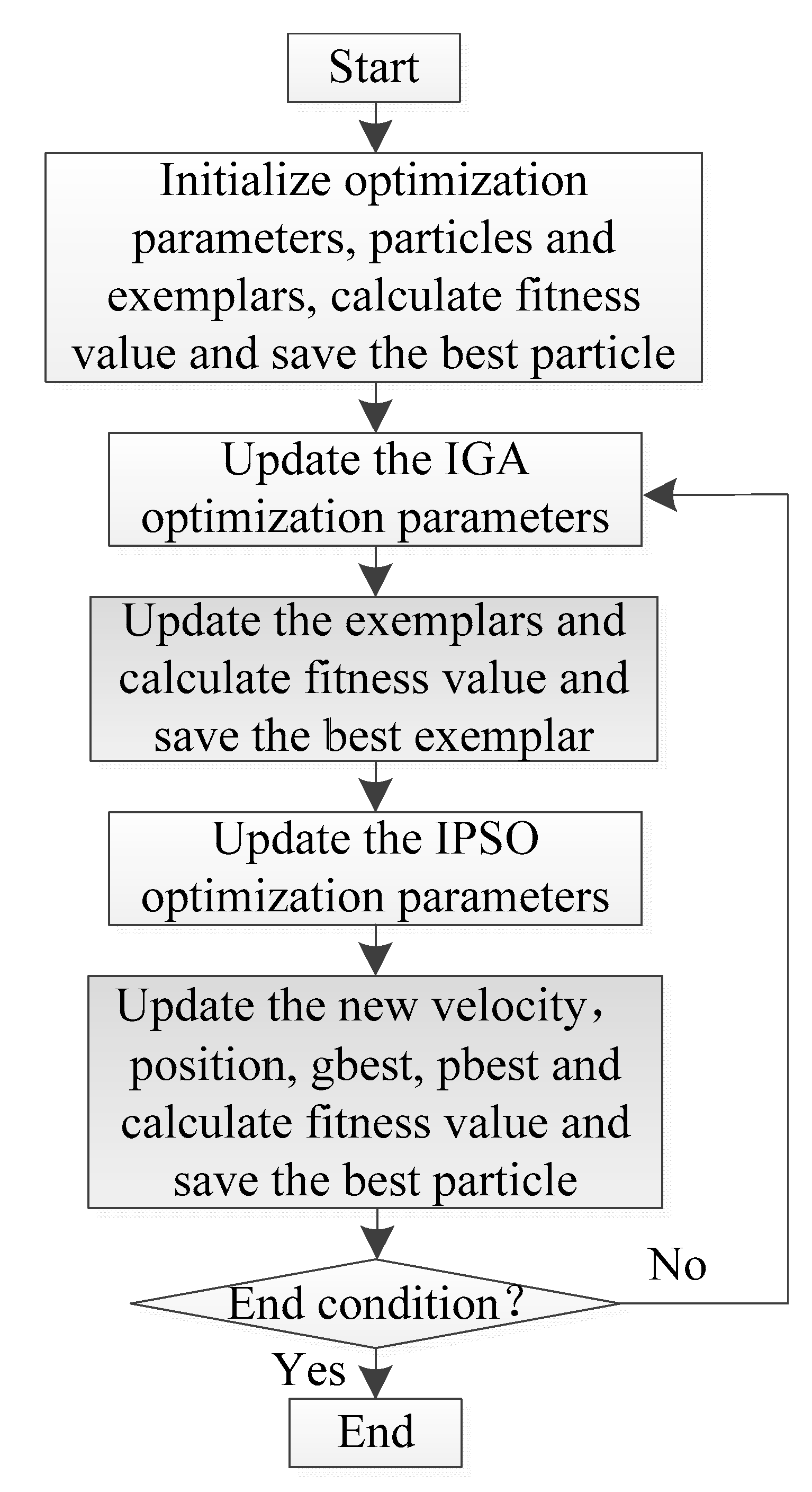
4.2. Parameters Identification Algorithm

In [27], a novel GLPSO hybrid algorithm with cascade structure using a single exemplary is proposed. However, in GLPSO hybrid algorithm, the inertia weight coefficient $\omega$, acceleration coefficient $c$ and crossover and mutation probabilities $P_c$ and $P_m$ are all constant. In view of this deficiency, the improved GA (IGA) and improved PSO (IPSO), which are derived from standard GA and PSO, are combined with GLPSO to further accelerate the convergence rate in this paper. The procedures of the improved GLPSO hybrid algorithm are shown in Figure 4. It includes the following 5 parts.

(1) The exemplar, velocity and location for each particle as well as population size, maximimal iterations and other parameters are initialized. The fitness value of each exemplar and particle is computed and the best particle is saved.

(2) The optimization parameters of IGA are updated according to (19), (20) [18]:

$$P_c^i=P_c^{i-1}+\frac{0.5-P_{c0}}{N}$$

(19)

where $P_c^i$ is crossover probability at the $i^{th}$ iteration. $P_{c0}$ is the initial crossover probability. $N$ is maximal number of iterations.

The recommended value range of mutation probability $P_m$ is 0.001–0.1. The $P_m$ is adjusted according to (20) [14].

$$\{\begin{array}{l}{P}_m^i=P_m^{i-1}+\frac{0.001-P_m^0}{N}\begin{array}{cc}& \mathrm{if}\tau =0\end{array}\\ P_m^i=P_m^0\begin{array}{cc}& \mathrm{if}\tau =1\end{array}\end{array}$$

(20)

where $\tau$ is a binary denoting whether reseting $P_m^i$ to the initial value $P_m^0$.

(3) Each exemplar is updated using IGA operation with the genetic materials gbest and pbest. Then, the objective function is computedfor each exemplar. After that, the optimal value and corresponding exemplar are saved.

(4) After IGA operation, the inertia weight coefficient $\omega$, acceleration coefficient $c$ are updated as follows.

$$\omega ={\omega }_{\max }-\left({\omega }_{\max }-{\omega }_{\min }\right)\times {\left(\frac{i}{N}\right)}^2$$

(21)

$$c=\left(c_{\max }-c_{\min }\right)\times \frac{N-i}{N}+c_{\min }$$

(22)

where ${\omega }_{\max }$ and ${\omega }_{\min }$ are the upper and lower bound of $\omega$. $c_{\max }$ and $c_{\min }$ are the upper and lower bound of $c$.

(5) The IPSO method is adopted to update all the particles using the new exemplar. The gbest and pbest as well as objective function of every particle are computed. Then the optimal fitness value and corresponding particle is saved. If the end conditions are satisfied, the program is terminated. Otherwise, go to Step 2. The new iteration cycle starts.

5. Text Case

5.1. Configurations of Case

As shown in Figure 5, the detailed model of WECC benchmark system is used to test the capability of the proposed method. The physical and control system parameters of each PMSG wind turbine and the step up transformer are shown in Table 1 and Table 2 respectively. The system base capacity is chosen to be $S_{\mathrm{B}}=S_{\mathrm{eq}}=30$ MVA when all PMSG wind turbines are online. A three-phase short-circuit fault with 8 $\mathsf{\Omega }$ transition resistance lasting for 4 cycles is set at the middle L1. The simulation time last for 0.2 s. Population size and maximum iteration of GLPSO is set to 50 and 15 respectively. The parameters identification interval is shown in

Table 5. Identification intervals of parameters.

${\mathit{\psi }}_{\mathbf{PM}}$	${\mathit{K}}_{\mathbf{p}\mathbf{2}}$	${\mathit{K}}_{\mathbf{i}\mathbf{2}}$	${\mathit{K}}_{\mathbf{p}\mathbf{3}}$	${\mathit{K}}_{\mathbf{i}\mathbf{3}}$
[0.594–2.377]	[1.600–40.000]	[80.000–2000.000]	[0.166–4.150]	[1.000–25.000]

.

5.2. Text Results

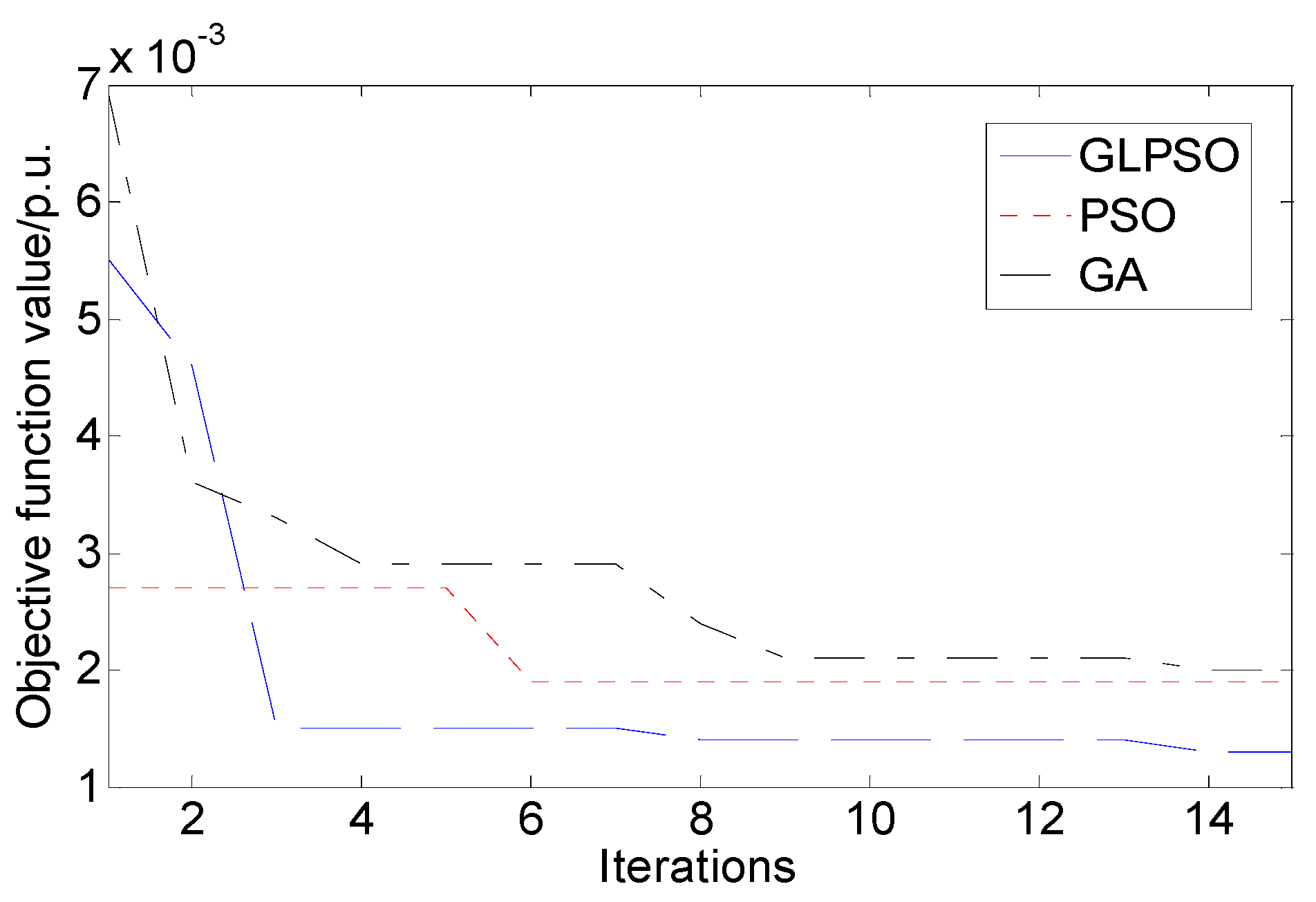
5.2.1. Convergence Rate and Searching Capability of Improved GLPSO

Set wind speed according to Table 5 in [22]. The value of objective function for 3 methods are shown in Figure 6. Clearly, the global searching capability of improved GLPSO is much higher than canonical PSO and GA. The reason is that the capability and convergence rate of GLPSO is much higher than PSO and GA, as well as the optimization coefficients are updated adaptively.

5.2.2. Dispersion of Identified Parameters

The results of identified parameters under various wind speeds and wake effect scenarios are shown in

Table 6. Parameter identification results 100% online.

Wind Speed	${\mathit{\psi }}_{\mathbf{PM}}$	${\mathit{K}}_{\mathbf{p}\mathbf{2}}$	${\mathit{K}}_{\mathbf{i}\mathbf{2}}$	${\mathit{K}}_{\mathbf{p}\mathbf{3}}$	${\mathit{K}}_{\mathbf{i}\mathbf{3}}$
7 m/s	1.5773	8.4326	358.5877	0.7698	3.7783
8 m/s	1.5580	8.1466	382.4388	0.7955	3.8919
9 m/s	1.7754	8.1307	417.8176	0.8106	4.8668
10 m/s	1.3471	7.9733	400.4220	0.8156	4.7120
11 m/s	1.4920	8.2924	364.5235	0.8159	5.6793
12 m/s	1.3722	7.9720	397.1256	0.8235	5.4453
Wake Effect	1.4550	7.7923	313.3526	0.7967	3.9189

. Clearly, the dispersion of $K_{\mathrm{p}2}$, $K_{\mathrm{p}3}$ is low. Other parameters have a certain degree of dispersion. Assume that the wind turbines 5, 9, 13, and 17 in Figure 5 are offline. The system base capacity is chosen to be $S_{\mathrm{B}}=S_{\mathrm{eq}}=30\times 0.8$ MVA. As shown in

Table 7. Results of parameters estimation 80% online.

Wind Speed	${\mathit{\psi }}_{\mathbf{PM}}$	${\mathit{K}}_{\mathbf{p}\mathbf{2}}$	${\mathit{K}}_{\mathbf{i}\mathbf{2}}$	${\mathit{K}}_{\mathbf{p}\mathbf{3}}$	${\mathit{K}}_{\mathbf{i}\mathbf{3}}$
7 m/s	1.5561	8.6378	257.2373	0.7594	4.3353
8 m/s	1.5625	8.3687	355.7341	0.7863	3.5676
9 m/s	1.7915	8.3210	395.7704	0.7889	3.8645
10 m/s	1.7601	8.2780	352.3386	0.8017	4.5689
11 m/s	1.5934	8.2248	432.2732	0.8155	5.5417
12 m/s	1.5880	8.1397	400.2451	0.8293	4.9157
Wake Effect	1.4849	7.7995	295.8272	0.8259	3.5769

, the dispersion of $K_{\mathrm{p}2}$ and $K_{\mathrm{p}3}$ is still low. As shown in Table 5 in [22], the wake effect is considered by setting wind speeds of each PMSG wind turbine different from each other. As shown in the last row in Table 6 and Table 7, the precision of parameter identification results for wake effect is slightly lower than other scenarios due to the large difference of operating states of each PMSG wind turbine. However, it is still satisfactory.

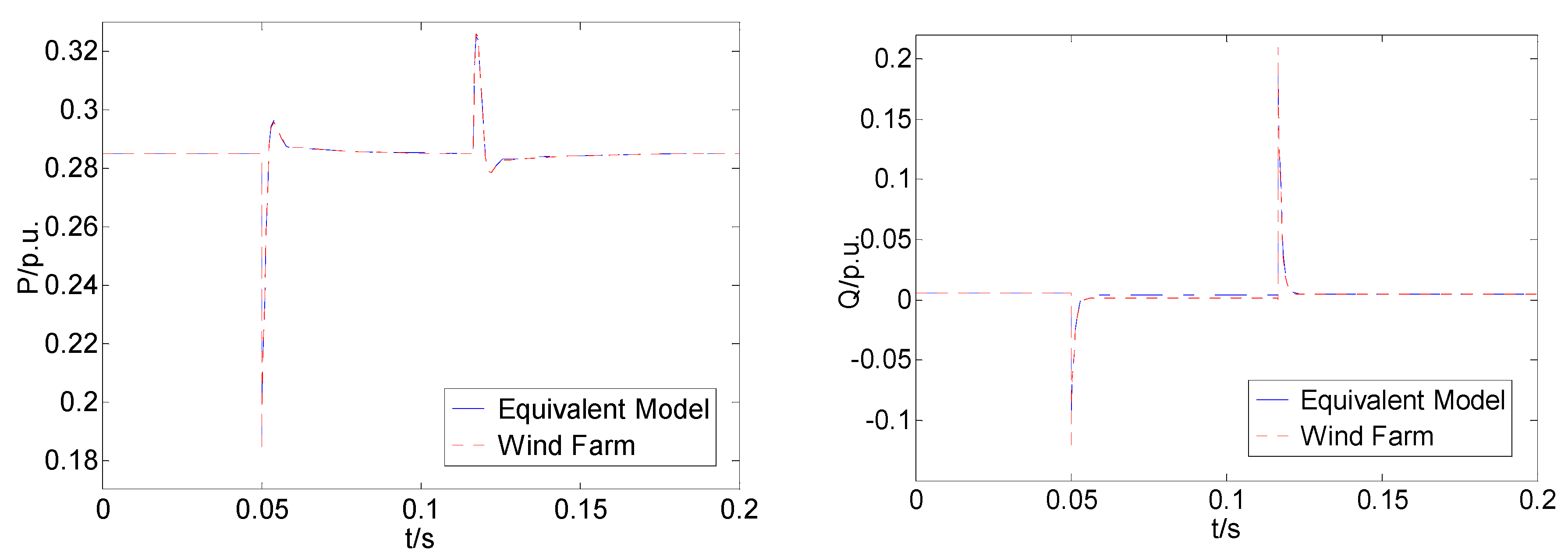
5.2.3. Verification of Descriptive Capability

The fitting curves when the wind speed of each turbine is set to 8 m/s, 9 m/s, 10 m/s, and 11 m/s are shown in Figure 7. Clearly, the output active and reactive power of the equivalent model overlaps those of wind farm respectively. Therefore, the equivalent model can describe dynamic characteristics of the wind farm after disturbance with very high precision.

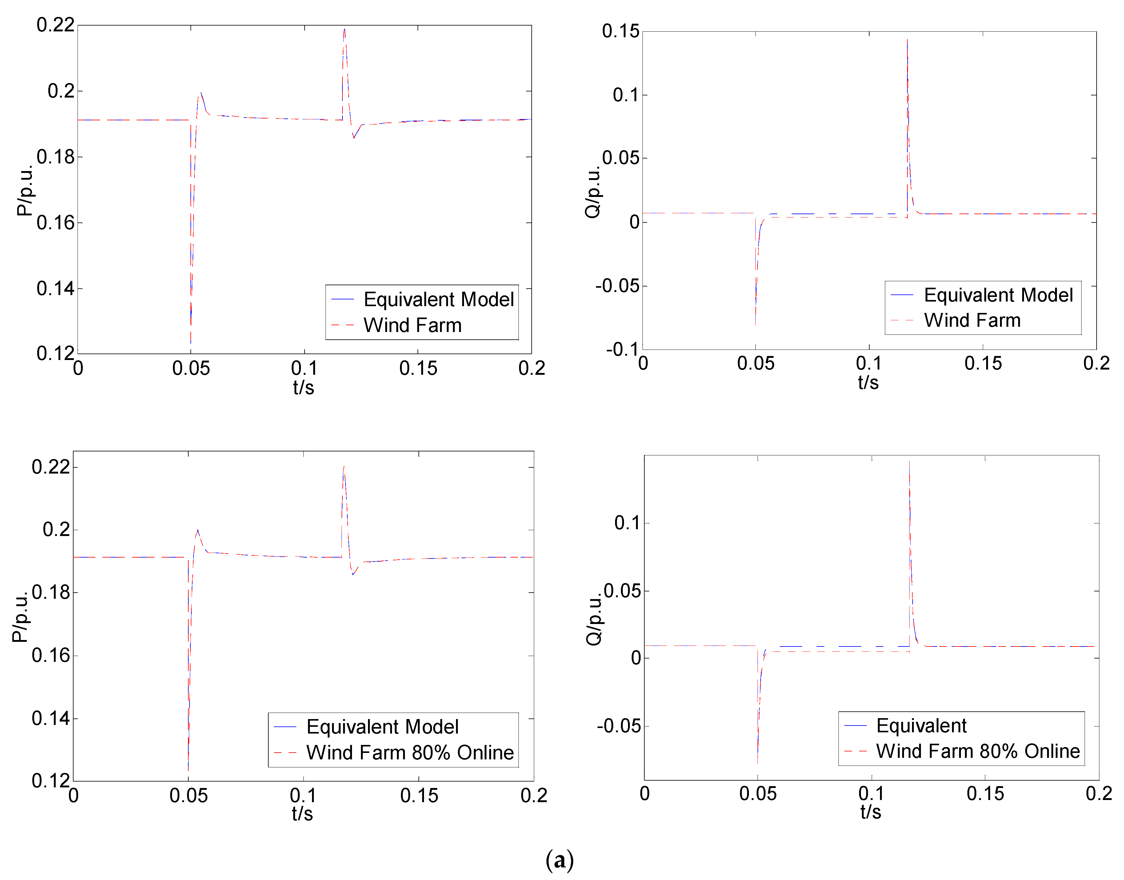
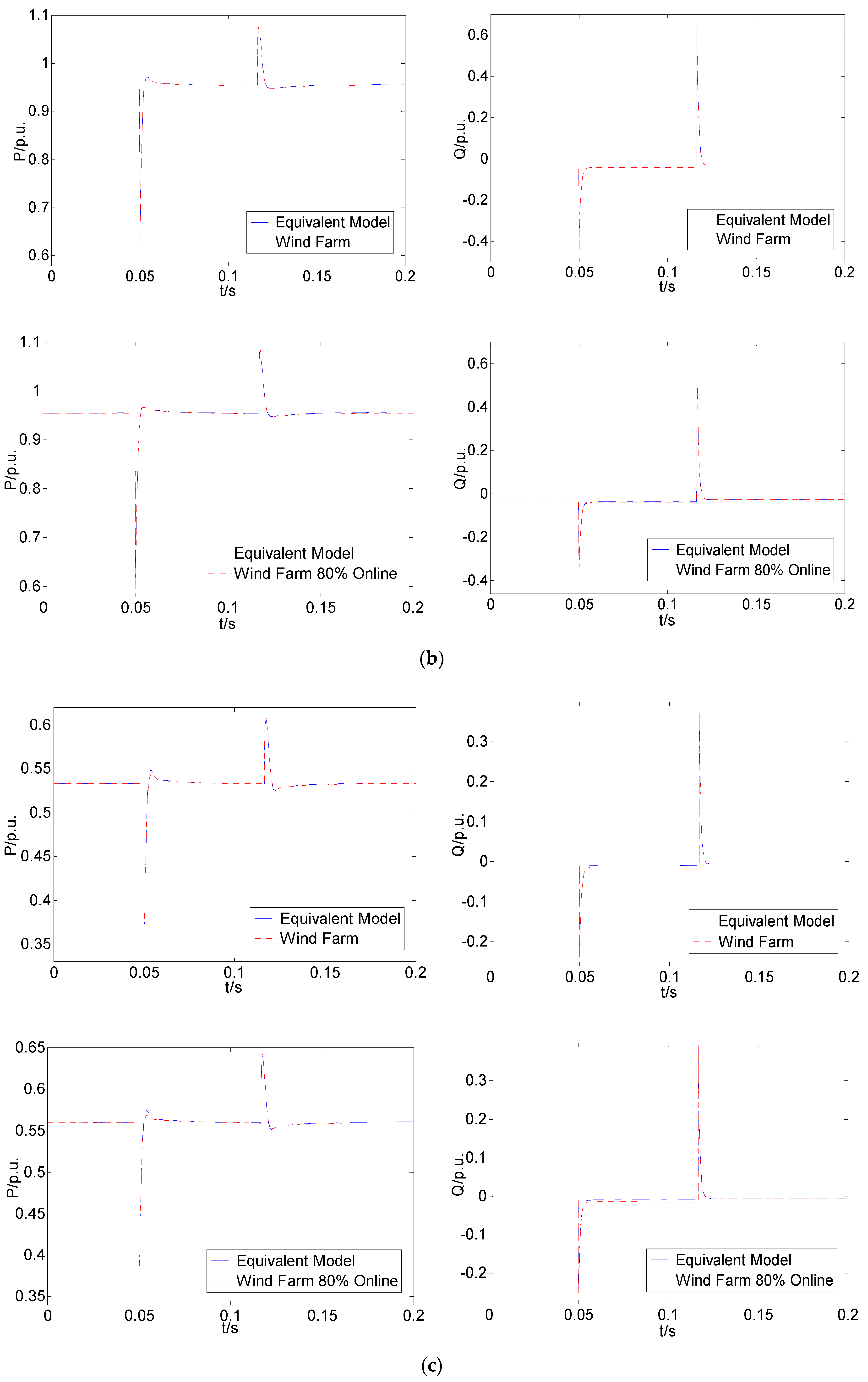
5.2.4. Verification of Generalization Capability

Equivalent model identified with 9 m/s wind speed is utilized to describe wind farm with 7 m/s, 12 m/s wind speed, under wake effect and 20% wind turbines are off line respectively. As shown in Figure 8, the deviation of output active and reactive power curves of the equivalent model from those of wind farm is very small, although the wind speeds differ much. As shown in

Table 8. Comparisons of fitting curves.

100% Online	Active Power	Reactive Power	80% Online	Active Power	Reactive Power
7 m/s	99.99%	99.75%	7 m/s	99.99%	99.59%
12 m/s	99.99%	99.98%	12 m/s	99.99%	99.98%
Wake Effect	99.94%	99.95%	Wake effect	99.93%	99.94%

, the goodness of fit [18] are very close to 100%. It concludes that the generalization capability of the proposed equivalent model and parameters identification strategy is high enough.

5.2.5. Unknown Wind Speed Scene

The results of parameters identification when wind speed is unknown are shown in

Table 9. Identification results when wind speed is unknown.

Parameters	${\mathit{\psi }}_{\mathbf{PM}}$	${\mathit{K}}_{\mathbf{p}\mathbf{2}}$	${\mathit{K}}_{\mathbf{i}\mathbf{2}}$	${\mathit{K}}_{\mathbf{p}\mathbf{3}}$	${\mathit{K}}_{\mathbf{i}\mathbf{3}}$
Wake Effect	1.5523	7.8411	279.2768	0.8237	3.9126

. Clearly, they are consistent with those in Table 6 and Table 7. It is worth pointing out that the identification results of ${\psi }_{\mathrm{PM}}$ in Table 6, Table 7 and Table 9 deviate a lot from the true value 1.1884. When the three-phase short-circuit transition resistance is set to 1 ohm, we have carried out the program of parameters identification many times. It is found that although other parameters cannot be identified precisely, $K_{\mathrm{p}3}$ and ${\psi }_{\mathrm{PM}}$ can be identified precisely. For all the programs, the mismatch between the identification results for ${\psi }_{\mathrm{PM}}$ and the true value 1.1884 are less than 5%. Further, the transient process time of power system is very short, generally within 10 s. The dynamic characteristics of PMSG wind farm depend on the regulating speed of GSC converter, which is generally in millisecond. As shown in Figure 7 and Figure 8, the transient process of PMSG wind farm is very short, far less than 0.2 s. In such a short period of time, the wind speed can be regarded as a constant value. The proposed method has good robustness and adaptability for the randomness of wind speed.

6. Conclusions

We show that the sensitivity of inertia time constant $T_{\mathrm{j}}$, stator reactance $L_{\mathrm{d}}$, $L_{\mathrm{q}}$ and proportional and integral amplification constant of current controller of MSC $K_{\mathrm{p}1}$, $K_{\mathrm{i}1}$ are very small after trajectory sensitivity analysis. Moreover, the phase of trajectory sensitivity for stator resistance $R_{\mathrm{s}}$ is opposite to permanent magnet flux linkage ${\psi }_{\mathrm{PM}}$. Simulation results using the WECC benchmark system indicate that the capability of the proposed improved GLPSO hybrid algorithm are much higher canonical PSO and GA. Further, the approach proposed is preferable to those in [20,24]. Because in [20] the parameters of PMSG wind farm are identified with load parameters. Since the sensitivity for parameters of load are much higher than parameters of a PMSG wind turbine, it is very difficult to identify the parameters of a PMSG wind turbine precisely if they are identified at the same time. Furthermore, the permanent magnet flux linkage of PMSG is not identified in [20], which has a significant impact on power system dynamics. Moreover, since the approach in [24] belongs to the aggregation method, detailed information of the whole wind farm is necessary. Furthermore, the method in [24] cannot be applicable after long-term operation of wind farm since the parameters of each PMSG wind turbine may deviate greatly from the values on the nameplate. Therefore, the proposed method is preferable to the on in [24] as well.

References

1. Mohammadpour, H.A.; Santi, E. SSR damping controller design and optimal placement in rotor-side and grid-side converters of series-compensated DFIG-based wind farm. IEEE Trans. Sustain. Energy 2015, 6, 388–399. [Google Scholar] [CrossRef]
2. Ullah, N.R.; Thiringe, T.; Karlsson, D. Voltage and transient stability support by wind farms complying with the E.ON Netz grid code. IEEE Trans. Power Syst. 2007, 22, 1647–1656. [Google Scholar] [CrossRef]
3. Kunjumuhammed, L.P.; Pal, B.C.; Gupta, R.; Dyke, K.J. Stability Analysis of a PMSG-Based Large Offshore Wind Farm Connected to a VSC-HVDC. IEEE Trans. Energy Convers. 2017, 32, 1166–1176. [Google Scholar] [CrossRef]
4. Song, R.; Guo, J.; Li, B.; Zhou, P.; Du, N.; Yang, D. Mechanism and characteristics of subsynchronous oscillation in direct-drive wind power generation system based on input-admittance analysis. Proc. CSEE 2017, 37, 4662–4670. [Google Scholar] [CrossRef]
5. Zhou, P.P.; Li, G.F.; Song, R.H.; Yang, D.Y. Subsynchronous oscillation characteristics and interactions of direct drive permanent magnet synchronous generator and static var generator. Proc. CSEE 2018, 38, 4369–4378. [Google Scholar] [CrossRef]
6. Xie, X.R.; Liu, H.K.; He, J.B.; Zhang, C.Y.; Qiao, Y. Mechanism and characteristics of subsynchronous oscillation caused by the interaction between full-converter wind turbines and AC systems. Proc. CSEE 2016, 36, 2366–2372. [Google Scholar] [CrossRef]
7. Ruan, J.-Y.; Lu, Z.-X.; Qiao, Y.; Min, Y. Analysis on Applicability Problems of the Aggregation-Based Representation of Wind Farms Considering DFIGs’ LVRT Behaviors. IEEE Trans. Power Syst. 2016, 31, 4953–4965. [Google Scholar] [CrossRef]
8. Wang, P.; Zhang, Z.; Huang, Q.; Wang, N.; Zhang, X.; Lee, W.-J. Improved Wind Farm Aggregated Modeling Method for Large-Scale Power System Stability Studies. IEEE Trans. Power Syst. 2018, 33, 6332–6342. [Google Scholar] [CrossRef]
9. Jalili-Marandi, V.; Pak, L.-F.; Dinavahi, V. Real-Time Simulation of Grid-Connected Wind Farms Using Physical Aggregation. IEEE Trans. Ind. Electron. 2009, 57, 3010–3021. [Google Scholar] [CrossRef]
10. Fernández, L.M.; Jurado, F.; Sáenz, J.R.; Fernández-Ramírez, L.M. Aggregated dynamic model for wind farms with doubly fed induction generator wind turbines. Renew. Energy 2008, 33, 129–140. [Google Scholar] [CrossRef]
11. Li, W.; Chao, P.; Liang, X.; Ma, J.; Xu, D.G.; Jin, X. A Practical Equivalent Method for DFIG Wind Farms. IEEE Trans. Sustain. Energy 2018, 9, 610–620. [Google Scholar] [CrossRef]
12. Ali, M.; Ilie, I.-S.; Milanovic, J.V.; Chicco, G. Wind Farm Model Aggregation Using Probabilistic Clustering. IEEE Trans. Power Syst. 2013, 28, 309–316. [Google Scholar] [CrossRef]
13. Zou, J.; Peng, C.; Xu, H.; Yan, Y. A Fuzzy Clustering Algorithm-Based Dynamic Equivalent Modeling Method for Wind Farm With DFIG. IEEE Trans. Energy Convers. 2015, 30, 1329–1337. [Google Scholar] [CrossRef]
14. Zhang, Y.; Muljadi, E.; Kosterev, D.; Singh, M. Wind Power Plant Model Validation Using Synchrophasor Measurements at the Point of Interconnection. IEEE Trans. Sustain. Energy 2014, 6, 984–992. [Google Scholar] [CrossRef]
15. Brochu, J.; LaRose, C.; Gagnon, R. Validation of Single- and Multiple-Machine Equivalents for Modeling Wind Power Plants. IEEE Trans. Energy Convers. 2010, 26, 532–541. [Google Scholar] [CrossRef]
16. Lin, J.; Cheng, L. Model Parameters Identification Method for Wind Farms Based on Wide-Area Trajectory Sensitivities. Int. J. Emerg. Electr. Power Syst. 2010, 11, 1–19. [Google Scholar] [CrossRef]
17. Cheng, X.; Lee, W.-J.; Sahni, M.; Cheng, Y.; Lee, L.K. Dynamic Equivalent Model Development to Improve the Operation Efficiency of Wind Farm. IEEE Trans. Ind. Appl. 2016, 52, 2759–2767. [Google Scholar] [CrossRef]
18. Wang, Y.; Lu, C.; Zhu, L.; Zhang, G.; Li, X.; Chen, Y. Comprehensive modeling and parameter identification of wind farms based on wide-area measurement systems. J. Mod. Power Syst. Clean Energy 2016, 4, 383–393. [Google Scholar] [CrossRef] [Green Version]
19. Kunjumuhammed, L.P.; Pal, B.C.; Oates, C.; Dyke, K.J. The Adequacy of the Present Practice in Dynamic Aggregated Modeling of Wind Farm Systems. IEEE Trans. Sustain. Energy 2016, 8, 23–32. [Google Scholar] [CrossRef] [Green Version]
20. Kim, D.-E.; El-Sharkawi, M.A. Dynamic Equivalent Model of Wind Power Plant Using Parameter Identification. IEEE Trans. Energy Convers. 2015, 31, 37–45. [Google Scholar] [CrossRef]
21. Zhou, Y.; Zhao, L.; Lee, W.-J. Robustness Analysis of Dynamic Equivalent Model of DFIG Wind Farm for Stability Study. IEEE Trans. Ind. Appl. 2018, 54, 5682–5690. [Google Scholar] [CrossRef]
22. Zhang, J.; Cui, M.; He, Y. Robustness and adaptability analysis for equivalent model of doubly fed induction generator wind farm using measured data. Appl. Energy 2020, 261, 1–12. [Google Scholar] [CrossRef]
23. Pan, X.; Feng, X.; Ju, P. Generalized load modeling of distribution network integrated with direct-drive permanent-magnet wind farms. Autom. Power Syst. 2017, 41, 62–68. [Google Scholar] [CrossRef]
24. Zhou, P.P.; Li, G.F.; Sun, H.D.; Song, R.H.; Du, N. Equivalent Modeling Method of PMSG Wind Farm Based on Frequency Domain Impedance Analysis. Proc. CSEE 2020, in press. [Google Scholar]
25. Xia, A.J.; Qiao, Y.; Lu, Z.X.; Ruan, J.Y. Effects of aggregated PMSG wind farm model error on transient stability analysis of power systems. Power Syst. Technol. 2016, 40, 341–347. [Google Scholar] [CrossRef]
26. Permanent Magnet Synchronous Generator (PMSG) Based Wind Power Generation System. Available online: https://www.mathworks.com/matlabcentral/fileexchange/36116-pmsg-based-wind-power-generation-system (accessed on 10 April 2012).
27. Gong, Y.J.; Li, J.-J.; Zhou, Y.; Li, Y.; Chung, H.S.-H.; Shi, Y.-H.; Zhang, J. Genetic Learning Particle Swarm Optimization. IEEE Trans. Cybern. 2015, 46, 2277–2290. [Google Scholar] [CrossRef] [PubMed] [Green Version]
Figure 1. Simulation system.
Energies 13 04607 g001
Figure 2. Trajectory sensitivity of active power when voltage dips about 30%: (a) Trajectory sensitivity of active power for R s and ψ PM ; (b) Trajectory sensitivity of active power for K p 2 , K i 2 , K p 3 and K i 3 .
Energies 13 04607 g002
Figure 3. Trajectory sensitivity of reactive power when voltage dips about 30%: (a)Trajectory sensitivity of reactive power for R s and ψ PM ; (b) Trajectory sensitivity of active power for K p 2 , K i 2 , K p 3 and K i 3 .
Energies 13 04607 g003
Figure 4. Flowchart of improved GLPSO algorithm.
Energies 13 04607 g004
Figure 5. 20 PMSG wind turbines system.
Energies 13 04607 g005
Figure 6. Comparison of three algorithms.
Energies 13 04607 g006
Figure 7. Descriptive capability of equivalent model: (a) comparison response for wind speed is 8 m/s; (b) comparison response for wind speed is 9 m/s; (c) comparison response for wind speed is 10 m/s; and (d) comparison response for wind speed is 11 m/s.
Energies 13 04607 g007aEnergies 13 04607 g007bEnergies 13 04607 g007c
Figure 8. Generalization ability of equivalent model: (a) comparison response for wind speed is 7 m/s; (b) comparison response for wind speed is 12 m/s; and (c) comparison response considering wake effect.
Energies 13 04607 g008aEnergies 13 04607 g008b