Power-Optimized Sinusoidal Piston Motion and Its Performance Gain for an Alpha-Type Stirling Engine with Limited Regeneration

 ,
, 
Abstract
1. Introduction
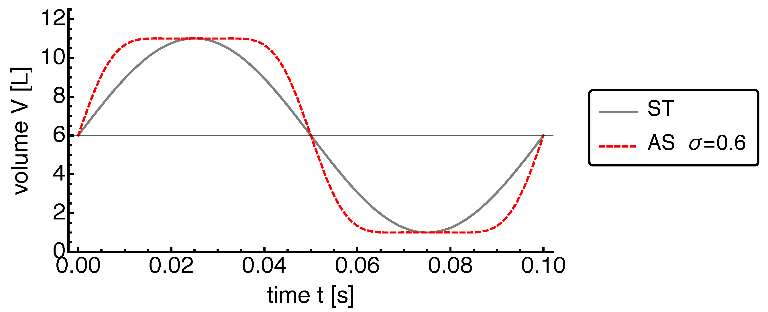
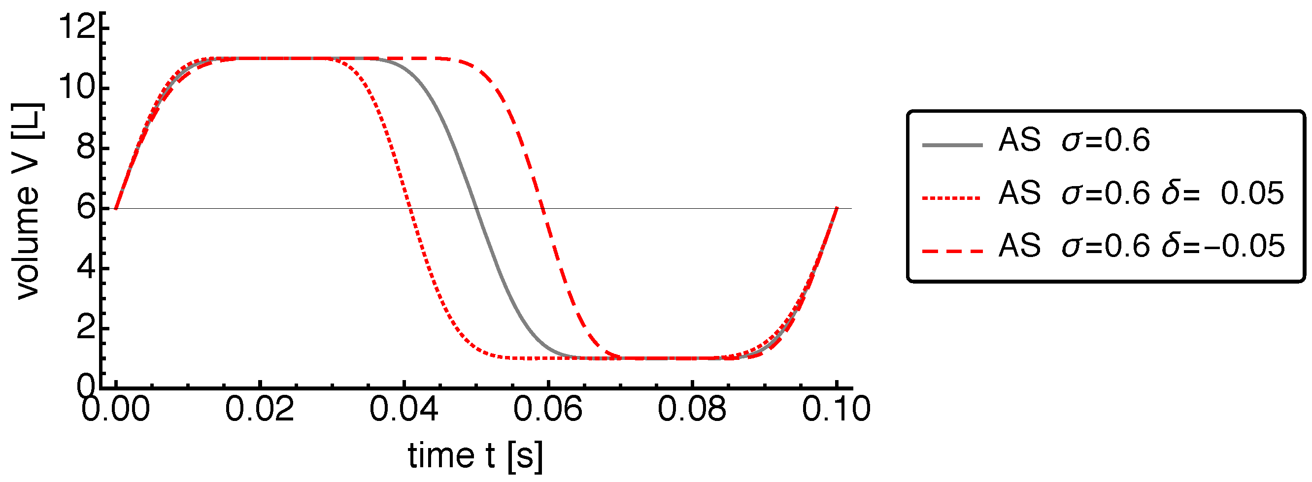
2. The AS Class of Piston Motions
3. Endoreversible Thermodynamics
4. The Stirling Engine Model
4.1. The Structure of the Endoreversible Stirling Engine Model
4.2. The Working Fluid
4.3. Heat Transfer
4.4. The Imperfect Regenerator
4.5. The Dynamics
4.6. Power Output, Efficiency and Entropy Production
5. Results
5.1. Power
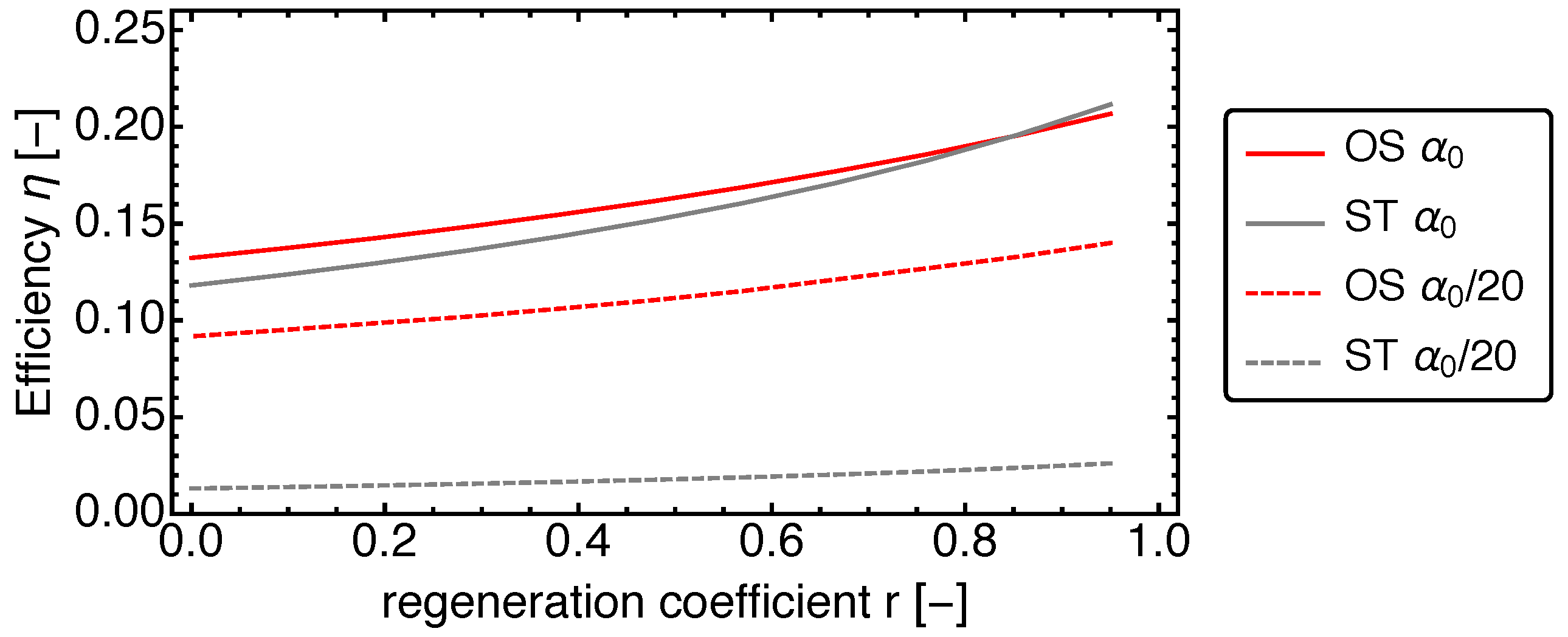
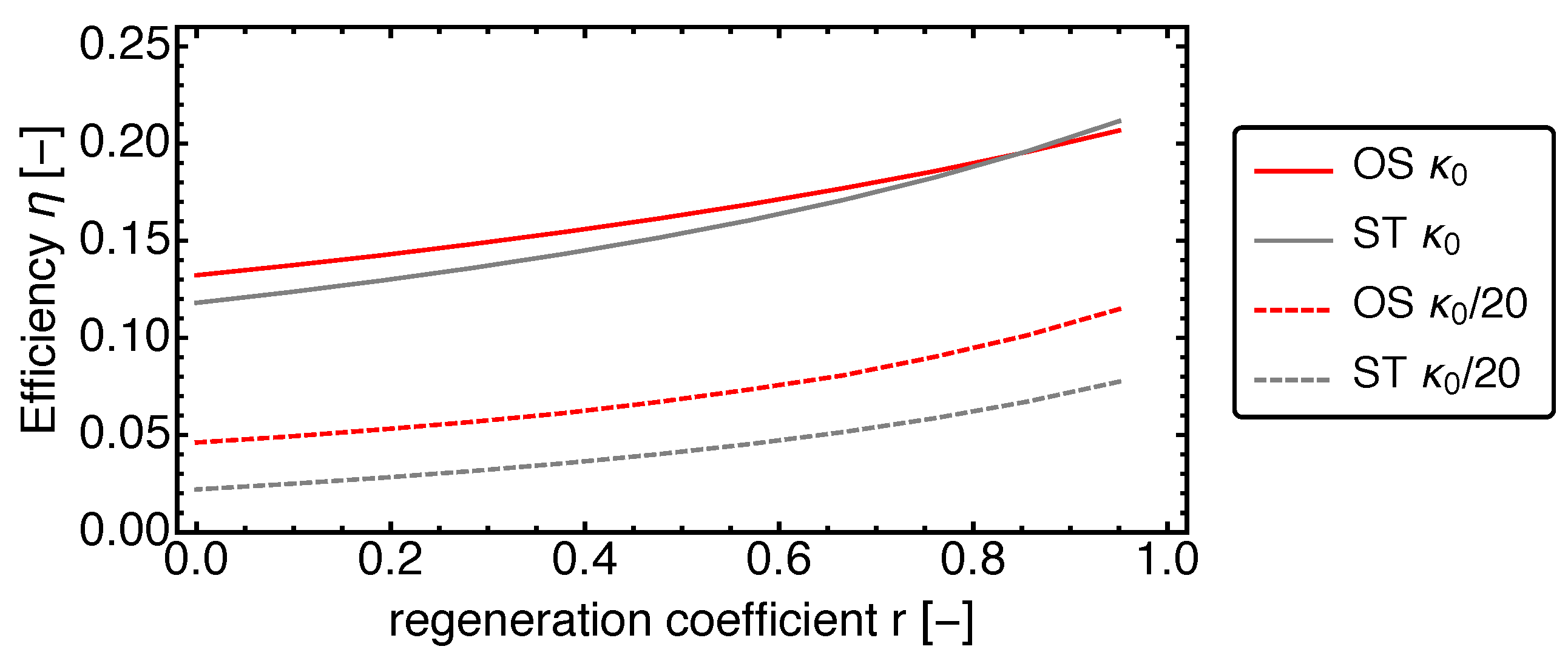
5.2. Efficiency
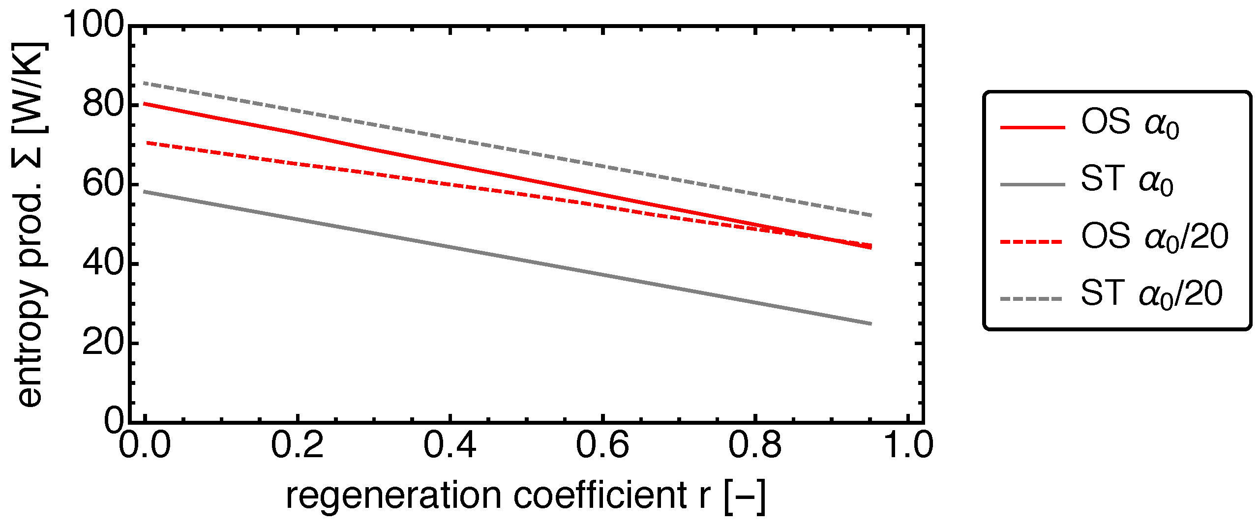
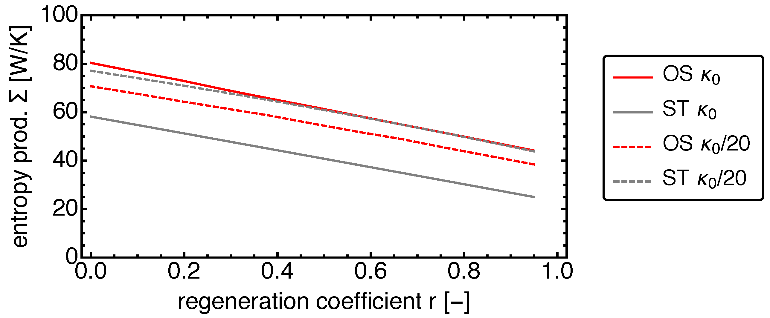
5.3. Entropy Production
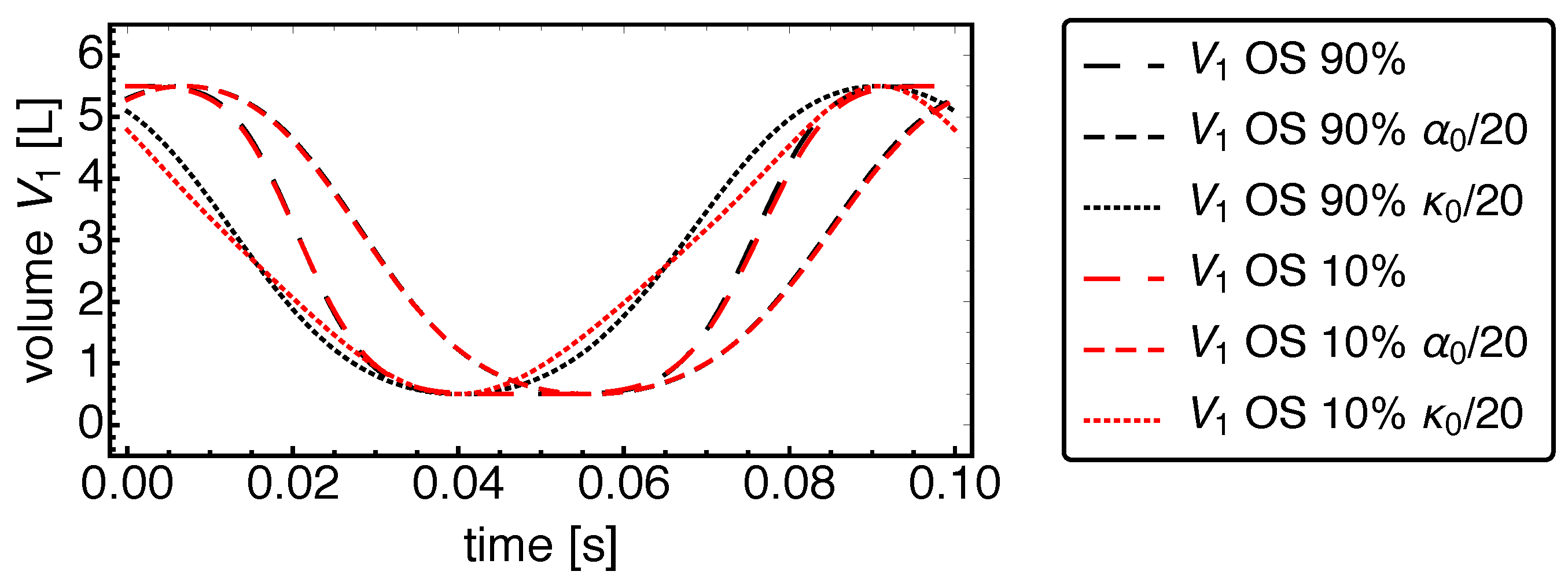
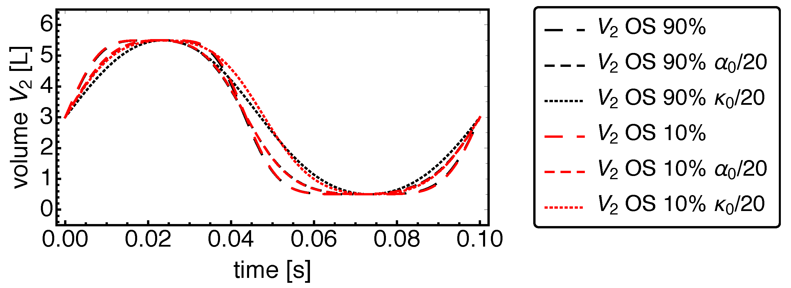
5.4. OS Piston Motion
6. Conclusions
Author Contributions
Funding
Conflicts of Interest
Nomenclature
| Greek symbols: | |
| Piston phase shift | |
| Piston time shift | |
| Mass transfer coefficient | |
| Mechanical friction coefficient | |
| Motion control parameter | |
| Efficiency | |
| Heat conductance | |
| Chemical potential | |
| Symbols: | |
| E | Energy |
| I | Flux of energy |
| J | Flux of extensity |
| Power | |
| R | Gas constant |
| S | Entropy |
| T | Temperature |
| U | Internal energy |
| V | Cylinder volume |
| Cylinder dead volume | |
| X | Extensity |
| Y | Intensity |
| Specific heat capacity | |
| h | Molar enthalpy |
| n | Mole number |
| p | Pressure |
| r | Regeneration coefficient |
| t | Time |
| Period of motion | |
| q | Heat flux |
| Subscripts: | |
| 0 | Reference |
| Piston number | |
| C, c | Cold |
| H, h | Hot |
| e | Environment |
| f | Friction |
| i | Subsystem |
| k | Contact point |
| r | Regenerator |
| Superscripts: | |
| Extensity type | |
| Abbreviations: | |
| AS | Adjustable sinusoidal motion |
| OS | Optimized sinusoidal motion |
| ST | Standard harmonic motion |
| SR | Entropy reservoir |
| WR, WT, WF | Work reservoirs |
References
- Stirling, R. Stirling Air Engine and the Heat Regenerator. British Patent 4081, 16 November 1816. [Google Scholar]
- Reader, G.T. Stirling Regenerators. Heat Transf. Eng. 1994, 15, 19–25. [Google Scholar] [CrossRef]
- Timoumi, Y.; Tlili, I.; Ben Nasrallah, S. Design and performance optimization of GPU-3 Stirling engines. Energy 2008, 33, 1100–1114. [Google Scholar] [CrossRef]
- Duan, C.; Wang, X.; Shu, S.; Jing, C.; Chang, H. Thermodynamic design of Stirling engine using multi-objective particle swarm optimization algorithm. Energ. Convers. Manag. 2014, 84, 88–96. [Google Scholar] [CrossRef]
- Hooshang, M.; Askari Moghadam, R.; Alizadeh Nia, S.; Tale Masouleh, M. Optimization of Stirling engine design parameters using neural networks. Renew. Energy 2015, 74, 855–866. [Google Scholar] [CrossRef]
- Ferreira, A.C.; Teixeira, S.; Teixeira, J.C.; Martins, L.B. Design Optimization of a Solar Dish Collector for Its Application With Stirling Engines. In Proceedings of the ASME 2015 International Mechanical Engineering Congress and Exposition, Houston, TX, USA, 13–19 November 2015. [Google Scholar] [CrossRef]
- Sowale, A.; Kolios, A.J. Thermodynamic Performance of Heat Exchangers in a Free Piston Stirling Engine. Energies 2018, 11, 505. [Google Scholar] [CrossRef]
- Sowale, A.; Anthony, E.J.; Kolios, A.J. Optimisation of a Quasi-Steady Model of a Free-Piston Stirling Engine. Energies 2019, 12, 72. [Google Scholar] [CrossRef]
- Mozurkewich, M.; Berry, R.S. Finite-time thermodynamics: Engine performance improved by optimized piston motion. Proc. Natl. Acad. Sci. USA 1981, 78, 1986–1988. [Google Scholar] [CrossRef]
- Hoffmann, K.H.; Watowich, S.J.; Berry, R.S. Optimal Paths for Thermodynamic Systems: The Ideal Diesel Cycle. J. Appl. Phys. 1985, 58, 2125–2134. [Google Scholar] [CrossRef]
- Huleihil, M.; Andresen, B. Optimal piston trajectories for adiabatic processes in the presence of friction. J. Appl. Phys. 2006, 100, 114914. [Google Scholar] [CrossRef]
- Huleihil, M. Optimal Stroke Path for Reciprocating Heat Engines. Modell. Simul. Eng. 2019, 2019, 7468478. [Google Scholar] [CrossRef]
- Chen, L.; Ma, K.; Ge, Y.; Feng, H. Re-Optimization of Expansion Work of a Heated Working Fluid with Generalized Radiative Heat Transfer Law. Entropy 2020, 22, 720. [Google Scholar] [CrossRef]
- Mozurkewich, M.; Berry, R.S. Optimal Paths for Thermodynamic Systems: The ideal Otto Cycle. J. Appl. Phys. 1982, 53, 34–42. [Google Scholar] [CrossRef]
- Xia, S.; Chen, L.; Sun, F. Maximum power configuration for multireservoir chemical engines. J. Appl. Phys. 2009, 105, 1–6. [Google Scholar] [CrossRef]
- Ge, Y.; Chen, L.; Sun, F. Optimal path of piston motion of irreversible Otto cycle for minimum entropy generation with radiative heat transfer law. J. Energy Inst. 2012, 85, 140–149. [Google Scholar] [CrossRef]
- Chen, L.; Xia, S.; Sun, F. Optimizing piston velocity profile for maximum work output from a generalized radiative law Diesel engine. Math. Comput. Model. 2011, 54, 2051–2063. [Google Scholar] [CrossRef]
- Xia, S.; Chen, L.; Sun, F. Engine performance improved by controlling piston motion: Linear phenomenological law system Diesel cycle. Int. J. Therm. Sci. 2012, 51, 163–174. [Google Scholar] [CrossRef]
- Lin, J.; Chang, S.; Xu, Z. Optimal motion trajectory for the four-stroke free-piston engine with irreversible Miller cycle via a Gauss pseudospectral method. J. Non-Equilib. Thermodyn. 2014, 39, 159–172. [Google Scholar] [CrossRef]
- Kojima, S. Theoretical Evaluation of the Maximum Work of Free-Piston Engine Generators. J. Non-Equilib. Thermodyn. 2017, 42, 31–58. [Google Scholar] [CrossRef]
- Watowich, S.J.; Hoffmann, K.H.; Berry, R.S. Optimal Paths for a Bimolecular, Light-Driven Engine. Il Nuovo Cim. B 1989, 104, 131–147. [Google Scholar] [CrossRef]
- Ma, K.; Chen, L.; Sun, F. Optimal paths for a light-driven engine with a linear phenomenological heat transfer law. Sci. China Chem. 2010, 53, 917–926. [Google Scholar] [CrossRef]
- Chen, L.; Ma, K.; Ge, Y. Optimal Configuration of a Bimolecular, Light-Driven Engine for Maximum Ecological Performance. Arab. J. Sci. Eng. 2017, 38, 341–350. [Google Scholar] [CrossRef]
- Kojima, S. Maximum Work of Free-Piston Stirling Engine Generators. J. Non-Equilib. Thermodyn. 2017, 42, 169–186. [Google Scholar] [CrossRef]
- Craun, M.; Bamieh, B. Optimal Periodic Control of an Ideal Stirling Engine Model. J. Dyn. Syst. Meas. Control 2015, 137, 071002. [Google Scholar] [CrossRef]
- Craun, M.J. Modeling and Control of an Actuated Stirling Engine. Ph.D Thesis, University of California, Santa Barbara, CA, USA, 2015. Available online: https://escholarship.org/uc/item/2tk2v9kj (accessed on 1 September 2020).
- Masser, R.; Khodja, A.; Scheunert, M.; Schwalbe, K.; Fischer, A.; Paul, R.; Hoffmann, K.H. Optimized Piston Motion for an Alpha-Type Stirling Engine. Entropy 2020, 22, 700. [Google Scholar] [CrossRef]
- Andresen, B.; Berry, R.S.; Nitzan, A.; Salamon, P. Thermodynamics in Finite Time. I. The Step-Carnot Cycle. Phys. Rev. A 1977, 15, 2086–2093. [Google Scholar] [CrossRef]
- Salamon, P.; Andresen, B.; Berry, R.S. Thermodynamics in Finite Time. II. Potentials for Finite-Time Processes. Phys. Rev. A 1977, 15, 2094–2102. [Google Scholar] [CrossRef]
- Andresen, B.; Salamon, P.; Berry, R.S. Thermodynamics in finite time: Extremals for imperfect heat engines. J. Chem. Phys. 1977, 66, 1571–1577. [Google Scholar] [CrossRef]
- Andresen, B.; Salamon, P.; Berry, R.S. Thermodynamics in Finite Time. Phys. Today 1984, 37, 62–70. [Google Scholar] [CrossRef]
- Hoffmann, K.H.; Burzler, J.M.; Schubert, S. Endoreversible Thermodynamics. J. Non-Equilib. Thermodyn. 1997, 22, 311–355. [Google Scholar]
- Hoffmann, K.H.; Burzler, J.M.; Fischer, A.; Schaller, M.; Schubert, S. Optimal Process Paths for Endoreversible Systems. J. Non-Equilib. Thermodyn. 2003, 28, 233–268. [Google Scholar] [CrossRef]
- Hoffmann, K.H. An introduction to endoreversible thermodynamics. AAPP Phys. Math. Nat. Sci. 2008, 86, 1–19. [Google Scholar] [CrossRef]
- Rubin, M.H. Optimal Configuration of a Class of Irreversible Heat Engines. I. Phys. Rev. A 1979, 19, 1272–1276. [Google Scholar] [CrossRef]
- Rubin, M.H.; Andresen, B. Optimal Staging of Endoreversible Heat Engines. J. Appl. Phys. 1982, 53, 1–7. [Google Scholar] [CrossRef]
- De Vos, A. Reflections on the power delivered by endoreversible engines. J. Phys. D Appl. Phys. 1987, 20, 232–236. [Google Scholar] [CrossRef]
- Chen, J.; Yan, Z. Optimal Performance of an Endoreversible-Combined Refrigeration Cycle. J. Appl. Phys. 1988, 63, 4795–4798. [Google Scholar] [CrossRef]
- Bǎdescu, V. On the Theoretical Maximum Efficiency of Solar-Radiation Utilization. Energy 1989, 14, 571–573. [Google Scholar] [CrossRef]
- De Vos, A. Is a solar cell an edoreversible engine? Sol. Cells 1991, 31, 181–196. [Google Scholar] [CrossRef]
- Schwalbe, K.; Hoffmann, K.H. Optimal Control of an Endoreversible Solar Power Plant. J. Non-Equilib. Thermodyn. 2018, 43, 255–271. [Google Scholar] [CrossRef]
- Schwalbe, K.; Hoffmann, K.H. Novikov engine with fluctuating heat bath temperature. J. Non-Equilib. Thermodyn. 2018, 43, 141–150. [Google Scholar] [CrossRef]
- Andresen, B.; Salamon, P. Distillation by Thermodynamic Geometry. In Thermodynamics of Energy Conversion an Transport; Sieniutycz, S., De Vos, A., Eds.; Springer: New York, NY, USA, 2000. [Google Scholar]
- Wagner, K.; Hoffmann, K.H. Endoreversible modeling of a PEM fuel cell. J. Non-Equilib. Thermodyn. 2015, 40, 283–294. [Google Scholar] [CrossRef]
- Tsirlin, A.; Sukin, I.A.; Balunov, A.; Schwalbe, K. The Rule of Temperature Coefficients for Selection of Optimal Separation Sequence for Multicomponent Mixtures in Thermal Systems. J. Non-Equilib. Thermodyn. 2017, 42, 359–369. [Google Scholar] [CrossRef]
- Marsik, F.; Weigand, B.; Thomas, M.; Tucek, O.; Novotny, P. On the Efficiency of Electrochemical Devices from the Perspective of Endoreversible Thermodynamics. J. Non-Equilib. Thermodyn. 2019, 44, 425–437. [Google Scholar] [CrossRef]
- Fischer, A.; Hoffmann, K.H. Can a quantitative simulation of an Otto engine be accurately rendered by a simple Novikov model with heat leak? J. Non-Equilib. Thermodyn. 2004, 29, 9–28. [Google Scholar] [CrossRef]
- Ding, Z.; Chen, L.; Sun, F. Finite time exergoeconomic performance for six endoreversible heat engine cycles: Unified description. Appl. Math. Mod. 2011, 35, 728–736. [Google Scholar] [CrossRef]
- Paéz-Hernández, R.T.; Chimal-Eguía, J.C.; Sánchez-Salas, N.; Ladino-Luna, D. General Properties for an Agrowal Thermal Engine. J. Non-Equilib. Thermodyn. 2018, 43, 131–139. [Google Scholar] [CrossRef]
- Masser, R.; Hoffmann, K.H. Dissipative Endoreversible Engine with Given Efficiency. Entropy 2019, 21, 1117. [Google Scholar] [CrossRef]
- Açıkkalp, E.; Yamık, H. Modeling and optimization of maximum available work for irreversible gas power cycles with temperature dependent specific heat. J. Non-Equilib. Thermodyn. 2015, 40, 25–39. [Google Scholar] [CrossRef]
- Masser, R.; Hoffmann, K.H. Endoreversible Modeling of a Hydraulic Recuperation System. Entropy 2020, 22, 383. [Google Scholar] [CrossRef]
- De Vos, A. Endoreversible Models for the Thermodynamics of Computing. Entropy 2020, 22, 660. [Google Scholar] [CrossRef]
- Schwalbe, K.; Hoffmann, K.H. Stochastic Novikov Engine with Fourier Heat Transport. J. Non-Equilib. Thermodyn. 2019, 44, 417–424. [Google Scholar] [CrossRef]
- Curzon, F.L.; Ahlborn, B. Efficiency of a Carnot Engine at Maximum Power Output. Am. J. Phys. 1975, 43, 22–24. [Google Scholar] [CrossRef]
- Wagner, K.; Hoffmann, K.H. Chemical reactions in endoreversible thermodynamics. Eur. J. Phys. 2016, 37, 015101. [Google Scholar] [CrossRef]
- Kuehl, H.D.; Schulz, S. A 2nd order regenerator model including flow dispersion and bypass losses. In Proceedings of the IECEC 96, 31st Intersociety Energy Conversion Engineering Conference, Washington, DC, USA, 11–16 August 1996; Volume 2, pp. 1343–1348. [Google Scholar]
- Nelder, J.A.; Mead, R. A Simplex Method for Function Minimization. Comput. J. 1965, 7, 308–313. [Google Scholar] [CrossRef]


© 2020 by the authors. Licensee MDPI, Basel, Switzerland. This article is an open access article distributed under the terms and conditions of the Creative Commons Attribution (CC BY) license (http://creativecommons.org/licenses/by/4.0/).
Share and Cite
Scheunert, M.; Masser, R.; Khodja, A.; Paul, R.; Schwalbe, K.; Fischer, A.; Hoffmann, K.H. Power-Optimized Sinusoidal Piston Motion and Its Performance Gain for an Alpha-Type Stirling Engine with Limited Regeneration. Energies 2020, 13, 4564. https://doi.org/10.3390/en13174564
Scheunert M, Masser R, Khodja A, Paul R, Schwalbe K, Fischer A, Hoffmann KH. Power-Optimized Sinusoidal Piston Motion and Its Performance Gain for an Alpha-Type Stirling Engine with Limited Regeneration. Energies. 2020; 13(17):4564. https://doi.org/10.3390/en13174564
Chicago/Turabian StyleScheunert, Mathias, Robin Masser, Abdellah Khodja, Raphael Paul, Karsten Schwalbe, Andreas Fischer, and Karl Heinz Hoffmann. 2020. "Power-Optimized Sinusoidal Piston Motion and Its Performance Gain for an Alpha-Type Stirling Engine with Limited Regeneration" Energies 13, no. 17: 4564. https://doi.org/10.3390/en13174564
APA StyleScheunert, M., Masser, R., Khodja, A., Paul, R., Schwalbe, K., Fischer, A., & Hoffmann, K. H. (2020). Power-Optimized Sinusoidal Piston Motion and Its Performance Gain for an Alpha-Type Stirling Engine with Limited Regeneration. Energies, 13(17), 4564. https://doi.org/10.3390/en13174564