Method for Clustering Daily Load Curve Based on SVD-KICIC

Abstract

Clustering electric load curves is an important part of the load data mining process. In this paper, we propose a clustering algorithm by combining singular value decomposition and KICIC clustering algorithm (SVD-KICIC) for analyzing the characteristics of daily load curves to mitigate some of the traditional clustering algorithm problems, such as only considering intra-class distance and low computational efficiency when dealing with massive load data. Our method identifies effective daily load curve characteristics using the singular value decomposition technique to improve dimensionality reduction, which improves low computational efficiency by reducing the number of dimensions inherent in big data. Additionally, the method performs SVD on the load data to obtain singular values for determination of weight of the KICIC algorithm, which leverages intra-class and inter-class distances of the load data and further improves the computational efficiency of the algorithm. Finally, we perform a series of simulations of actual load curves from a certain city to validate that the algorithm proposed in this paper has a short operation time, high clustering quality, and solid robustness that improves the clustering performance of the load curves.

1. Introduction

In recent years, with growing demand for electricity and the popularized use of smart electricity meters, electric power systems have accumulated increasingly massive load data [1,2]. However, the load demand response has many characteristics such as complexity, randomness and high non-linearity. By using load data mining and identifying electricity consumption modes, users’ electricity consumption characteristics can be obtained and used to provide an important reference for the reliable operation of the power grids, to refine user partitioning and to personalize interactions between the electric power systems and users [3,4,5].

Clustering algorithms are an effective approach to mining the electricity consumption characteristics of users [6,7]. Common clustering algorithms are primarily hierarchical, partition-based, grid-based or model-based [8]. In existing research, most of the clustering algorithms specific to load curves use distance similarity for classification. In [9], the major characteristics of the daily load curves are extracted for clustering by combining the principal component analysis method and the K-means algorithm. In [10], a load classification method based on the Gaussian mixture model and multi-dimensional analysis is developed. In this method, the load data are subject to multi-dimensional analysis and dimensionality reduction; then, the resulting data are used with the Gaussian mixture model clustering algorithm for the classification of large-scale load data sets. In [11], an integrated clustering algorithm is developed by comparing the advantages and disadvantages of multiple clustering algorithms. The resulting algorithm effectively combines the K-means algorithm and the hierarchical clustering algorithm. In [12], major characteristics are obtained by singular value decomposition (SVD) for dimensionality reduction and to perform weighted K-means clustering of the load curves. In [13], six daily load characteristic indexes are selected as dimensionality reduction indexes to express the original load curves before clustering, thus improving clustering efficiency. However, these methods only consider minimizing intra-class distance for improving the intra-class compactness and ignore the effects of the inter-class distance on the clustering results when they use distance as the daily load curve similarity measure for clustering. The methods’ clustering results tend to have a blurred boundary, and the load curves at various types of boundaries might be categorized incorrectly, thus leading to lower clustering quality. In addition, the existence of blurred samples might result in an increase in the number of iterations of the algorithm and a decrease in computational efficiency.

In response to the decrease in clustering quality due to inter-class blurred samples, in [14], the ESSC (enhanced soft subspace clustering) algorithm is proposed, which expands the inter-class distance by maximizing the distance between various centers and the global center. However, this method makes the shift of the class center unsatisfactory. Especially when inter-class distribution in clustering samples is nonuniform, maximizing the distance between the global center and the various class centers might cause several closer class centers to be more compact, which contradicts the original purpose of maximizing the inter-class distance and weakens the clustering effect. In [15], to further improve the clustering quality, the weighted K-means algorithm in combination with the intra-cluster and inter-cluster distances (KICIC) is proposed. The algorithm adds inter-class distance to the traditional weighted K-means algorithm and maximizes the distance between the class center and samples of other classes, reducing the effects of boundary samples on the clustering results. However, the method requires iteratively updating the weights of various dimensions, which occupies large computational resources. In particular, its computational efficiency for massive data has to be improved.

Comprehensively considering all the reviewed clustering methods, we propose a clustering algorithm based on SVD-KICIC to deal with the problems of low clustering quality and poor efficiency caused by blurred boundary samples in traditional clustering techniques for daily load curves. Our method performs dimensionality reduction of the original data by applying a singular value decomposition to the data then conducting a clustering analysis of the daily load curves by maximizing inter-class distance with a KICIC algorithm. Our method considers data obtained by sampling at each time point of the load curve as a dimension and extracts the dimensionality weighted via SVD dimensionality reduction, thus forming samples with weights of various dimensions to be clustered. The method establishes an objective function in combination with intra-class and inter-class distance, guaranteeing the minimum intra-class distance and the maximum inter-class distance, achieving effective and accurate clustering of load curves. The measured daily load data from a city are used as a sample here. They is compared against three clustering algorithms that do not consider inter-class distance, traditional K-means, SVD-weighted K-means, and KICIC algorithms, to verify the effectiveness and accuracy of the algorithm proposed in this paper.

2. Basic Principles

2.1. Theory of Singular Value Decomposition

We assume $X=\left[X_1,X_2,\cdots X_m\right]$ is a $m\times n$-order real matrix containing $m$ load curves, where the $i$th load curve is denoted as ${\mathit{X}}_i=\left[x_{i1},x_{i2},\cdots ,x_{in}\right]$ and $n$ is the number of sampling points of the load curve. The number of load curves for clustering analysis, $m$, is generally larger than $n$, the number of the sampling points. Thus, we let $m>n$ in this work.

The SVD technique decomposes the real matrix $X$ into three matrices [16,17]: $\mathit{U}$, $\mathit{\Lambda }$, and ${\mathit{V}}^{\mathrm{T}}$

$$\{\begin{array}{l}\mathit{X}=\mathit{U}\mathit{\Lambda }{\mathit{V}}^{\mathrm{T}}\\ \mathit{\Lambda }=\left[\begin{array}{c}{\mathit{\Lambda }}_1\\ 0\end{array}\right]\end{array}$$

(1)

where the orthogonal matrix $U=\left[u_1,u_2,\cdots ,u_m\right]$ is an $m\times m$-order matrix with each column vector being a mutually orthogonal unit vector. Meanwhile, the column vector is the characteristic vector of the matrix $X{X}^{\mathrm{T}}$ and called the left singular vector. The orthogonal matrix $V=\left[v_1,v_2,\cdots ,v_n\right]$ is an $n\times n$-order matrix, its column vector is also a mutually orthogonal unit vector. Meanwhile, it is the characteristic vector of the matrix $X{X}^{\mathrm{T}}$ and called the right singular vector. ${\Lambda }_1=\mathrm{diag}({\lambda }_1,{\lambda }_2,\cdots ,{\lambda }_n)$ is a diagonal matrix such that its diagonal elements are the singular values of the matrix $X$, which are decreasing in sequence (i.e., ${\lambda }_1\ge {\lambda }_2\ge \cdots \ge {\lambda }_n$). Equation (1) is expressed as

$$\begin{array}{ll}\mathit{X}& =\mathit{U}\mathit{\Lambda }{\mathit{V}}^{\mathrm{T}}\\ & =\left[u_1 u_2 \cdots u_m\right]\left[\begin{array}{c}{\mathit{\Lambda }}_1\\ 0\end{array}\right]{\left[v_1 v_2 \cdots v_n\right]}^{\mathrm{T}}=\\ & \left[{\lambda }_1{u}_1 {\lambda }_2{u}_2 \cdots {\lambda }_n{u}_n\right]\left[\begin{array}{l}{v}_1^{\mathrm{T}}\\ v_2^{\mathrm{T}}\\ ⋮\\ v_n^{\mathrm{T}}\end{array}\right]={\displaystyle \sum _{j=1}^n{\lambda }_j{u}_j{v}_j{}^{\mathrm{T}}}\end{array}$$

(2)

We consider a load curve ${\mathit{X}}_i$ in the matrix $\mathit{X}$ as an example. From Equation (2), we can derive

$$\begin{array}{c}{\mathit{X}}_i=\left[\begin{array}{cccc}{\lambda }_1{u}_{1i}& {\lambda }_2{u}_{2i}& \cdots & {\lambda }_n{u}_{ni}\end{array}\right]\mathbf{·}\\ {\left[\begin{array}{cccc}{v}_1{}^{\mathrm{T}}& v_2{}^{\mathrm{T}}& \cdots & v_n^{\mathrm{T}}\end{array}\right]}^{\mathrm{T}}\end{array}$$

(3)

where $u_{1i}$ is the coordinate of the vector ${\mathit{u}}_1$ at the first point and $u_{2i}$ is similarly defined.

Thus, the SVD method establishes a new orthogonal coordinate system with the vectors ${\mathit{v}}_1,{\mathit{v}}_2,\cdots ,{\mathit{v}}_n$ as the coordinate axes. The singular value ${\lambda }_j$ denotes the scale from the vector ${\mathit{u}}_j$ to the coordinate axis ${\mathit{v}}_j$; ${\lambda }_j{u}_{j,i}$ is the coordinate value of the load curve ${\mathit{X}}_i$ on the coordinate axis ${\mathit{v}}_j$. In addition, the larger the singular value ${\lambda }_j$, the greater the degree of data dispersion on the coordinate axis ${\mathit{v}}_j$, and the greater the variance of the data reflected, the better the coordinate axis can indicate the variation direction of the data. As the singular values obtained from the SVD method are arranged in descending order, the coordinate axes ${\mathit{v}}_1,{\mathit{v}}_2,\cdots ,{\mathit{v}}_q$ corresponding to the first $q$ singular values ${\lambda }_1,{\lambda }_2,\cdots ,{\lambda }_q$ are the $q$ major variation directions of the matrix, and can best represent the major characteristics of the original matrix. The matrix $\mathit{X}$ and the load curve ${\mathit{X}}_i$ can be approximately denoted as

$$\begin{array}{ll}\mathit{X}& \approx \mathit{Y}\mathbf{·}{\left[\begin{array}{cccc}{v}_1{}^{\mathrm{T}}& v_2{}^{\mathrm{T}}& \cdots & v_q{}^{\mathrm{T}}\end{array}\right]}^{\mathrm{T}}\\ & =\left[\begin{array}{cccc}{\lambda }_1{u}_1& {\lambda }_2{u}_2& \cdots & {\lambda }_q{u}_q\end{array}\right]\mathbf{·}\\ & {\left[\begin{array}{cccc}{v}_1{}^{\mathrm{T}}& v_2{}^{\mathrm{T}}& \cdots & v_q{}^{\mathrm{T}}\end{array}\right]}^{\mathrm{T}}\end{array}$$

(4)

$$\begin{array}{ll}{\mathit{X}}_i& \approx {\mathit{Y}}_i\mathbf{·}{\left[\begin{array}{cccc}{\mathit{v}}_1{}^{\mathrm{T}}& {\mathit{v}}_2{}^{\mathrm{T}}& \cdots & {\mathit{v}}_q{}^{\mathrm{T}}\end{array}\right]}^{\mathrm{T}}\\ & =\left[\begin{array}{cccc}{\lambda }_1{u}_{1i}& {\lambda }_2{u}_{2i}& \cdots & {\lambda }_q{u}_{qi}\end{array}\right]\mathbf{·}\\ & {\left[\begin{array}{cccc}{\mathit{v}}_1{}^{\mathrm{T}}& {\mathit{v}}_2{}^{\mathrm{T}}& \cdots & {\mathit{v}}_q{}^{\mathrm{T}}\end{array}\right]}^{\mathrm{T}}\end{array}$$

(5)

According to Equations (4) and (5), the major characteristics of the load curve ${\mathit{X}}_i$ can be denoted as ${\mathit{Y}}_i=\left[y_{i1},y_{i2},\cdots ,y_{iq}\right]$ in a low dimension coordinate system by reducing inessential coordinate axes.

2.2. Weighting K-Means Algorithm in Combination with the Intra-Class and Inter-Class Distance

The traditional K-means algorithm, and its derivative algorithms, generally use intra-class Euclidean distance as an indicator for judging similarity among daily load curves. However, in actual applications, the daily load curves usually have blurred inter-class samples. As shown in Figure 1, the load curves at the boundaries of various classes might be assigned to other classes, thus leading to low clustering quality. In addition, due to the existence of blurred samples, the number of algorithm iterations increases, thus reducing the computational efficiency.

In response to this problem, [15] proposes the KICIC clustering algorithm. As the traditional algorithm only considers the intra-class distance, this algorithm integrates inter-class distance, and maximizes inter-class distance while minimizing intra-class distance. Therefore, a target function is established:

$$\begin{array}{ll}P& =P(\mathit{U},\mathit{W},\mathit{Z})\\ & ={\displaystyle \sum _{p=1}^k{\displaystyle \sum _{i=1}^m{u}_{ip}{\displaystyle \sum _{j=1}^n{w}_{pj}{(x_{ij}-z_{pj})}^2}}}\\ & -\eta {\displaystyle \sum _{p=1}^k{\displaystyle \sum _{i=1}^m(1-u_{ip}){\displaystyle \sum _{j=1}^n{w}_{pj}{(x_{ij}-z_{pj})}^2}}}\\ & +\gamma {\displaystyle \sum _{p=1}^k{\displaystyle \sum _{j=1}^n{w}_{pj}\log w_{pj}}}\end{array}$$

(6)

and constraint condition:

$$\{\begin{array}{l}{\displaystyle \sum _{p=1}^k{u}_{ip}=1,u_{ip}\in \left\{0,1\right\}}\\ {\displaystyle \sum _{j=1}^n{w}_{pj}=1,0\le w_{pj}\le 1}\end{array}$$

(7)

where $\mathit{Z}=\left[{\mathit{Z}}_1,{\mathit{Z}}_2,\cdots ,{\mathit{Z}}_k\right]$ is the $k$ clustering centers with ${\mathit{Z}}_p=\left[z_{p1},z_{p2},\cdots ,z_{pq}\right]$ being the $p$th clustering center. $\mathit{W}=\left[{\mathit{W}}_1,{\mathit{W}}_2,\cdots ,{\mathit{W}}_k\right]$ is the $k$ weight vectors, with ${\mathit{W}}_p=\left[w_{p1},w_{p2},\cdots ,w_{pn}\right]$ being the weight of each sampling point in the $p$th class. When the $i$th load curve is assigned to the $p$th class, let $u_{ip}=1$, otherwise $u_{ip}=0$. Therefore, the $m\times k$ assignment matrix $\mathit{U}$ is constituted.

Minimizing target function (6) is the optimization principle, and the analysis is conducted on the basis of three items. The purpose of the first item is to minimize the intra-class distance of the sample in its class; the role of the second item is to maximize the inter-class distance; the third item adjusts the characteristic weight distribution via the entropy of weight. However, in actual applications, the KICIC algorithm occupies large computational resources when solving for the weight matrix $\mathit{W}$ [15]. Thus, the curse of dimensionality arises from this high-dimensionality data and results in low computational efficiency. In this work, we use the SVD technique for dimensionality reduction to improve the computational efficiency of the KICIC algorithm.

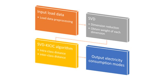
3. SVD-KICIC Algorithm

3.1. Data Preprocessing

3.1.1. Identification and Correction of Abnormal or Missing Data

As a series of problems may occur during the process of load data acquisition, such as communication interruption, measurement equipment failures, interference of environmental factors, and so on, the load data could be abnormal or even missing. When the amount of missing or abnormal data exceeds 10% (included) of the number of samples, the invalid curves need to be rejected. To improve the data quality, the load data need to be preprocessed prior to SVD. The load variation rate ${\delta }_{i,j}$ of a certain load curve ${\mathit{X}}_i=[x_{i,1},x_{i,2},\cdots ,x_{i,n}]$ is set as the basis. The abnormal data are evaluated using

$${\delta }_{i,j}=\frac{x_{i,j+1}-x_{i,j}}{x_{i,j}}$$

(8)

where ${\delta }_{i,j}$ is the load variation rate of the load curve ${\mathit{X}}_i$ at the $j$th sampling point. When the number of sampling points $n=$ 48, the threshold value $\epsilon$ generally ranges from 0.6 to 0.9. In other words, when ${\delta }_{i,j}\ge \epsilon$, the data at the sampling point are considered abnormal.

For abnormal data points, a smooth correction equation is used for correction and substitution:

$$x_{i,j}^{*}=\frac{{\displaystyle \sum _{g=1}^{g_1}{x}_{i,j-g}+{\displaystyle \sum _{h=1}^{h_1}{x}_{i,j+h}}}}{g_1+h_1}$$

(9)

where $x_{i,j}^{*}$ is the corrected value of the abnormal data point $x_{i,j}$, $g$ denotes a forward value assignment, $h$ denotes a backward value assignment, and values are assigned to $g_1$, $h_1$ according to the number of sampling points in the actual case, generally 4~7.

3.1.2. Load Curve Normalization

The amplitude values of the load data collected from different users may differ substantially. Direct clustering lacks objective accuracy, and the clustering results are unreliable if the load data does have the same order of magnitude before clustering. In this research, we process load data using the maximum value normalization principle. The processing method can be characterized by

$$x{\prime }_{i,j}=\frac{x_{i,j}}{\max ({\mathit{X}}_i)}$$

(10)

where $x{\prime }_{i,j}$ is the normalized data at the sampling point $j$ of the $i$th load curve. Then a new normalized matrix $\mathit{X}\prime$ is obtained with element $x{\prime }_{i,j}$.

3.2. SVD-KICIC and Its Implementation

A traditional KICIC algorithm uses the complete information of the samples as its input. Because of this, the computation is complex for larger sample sizes. In this work, we calculate the characteristic information matrix $\mathit{Y}$ using an SVD dimensionality reduction technique and use it as the input of the KICIC algorithm. Meanwhile, based on the singular values obtained by the SVD method, we redefine the weights of the KICIC algorithm and improve the overall clustering performance. The specific method is described in Section 3.2.

3.2.1. Improving the Target Function

The weight matrix $\mathit{W}=\left[{\mathit{W}}_1,{\mathit{W}}_2,\cdots ,{\mathit{W}}_k\right]$ in Equation (11) of the KICIC algorithm independently assigns weight vectors to the load data of each class. The value $w_{pj}$ denotes the weight value of the $j$th sampling point in the $p$th class. The algorithm needs to solve the assignment matrix $\mathit{U}$, clustering center matrix $\mathit{Z}$, and the weight matrix $\mathit{W}$, which consume large computational resources.

To improve the overall performance of the KICIC algorithm, we use the characteristic information matrix $\mathit{Y}$ obtained from SVD as the input, and use the weight vector $\mathit{W}\prime =\left[w{\prime }_1,w{\prime }_2,\cdots ,w{\prime }_q\right]$ obtained from normalization with the sum of the first $q$ singular values being 1 as the dimensionality weight of the information matrix, then propose the target function of the SVD-KICIC algorithm.

$$\begin{array}{ll}P& =P(\mathit{U},\mathit{Z})\\ & ={\displaystyle \sum _{p=1}^k{\displaystyle \sum _{i=1}^m{u}_{{}_{ip}}}{\displaystyle \sum _{j=1}^{q}w{\prime }_j{(y_{ij}-z_{pj})}^2}}\\ & -\eta {\displaystyle \sum _{p=1}^k{\displaystyle \sum _{i=1}^m(1-u_{ip}){\displaystyle \sum _{j=1}^{q}w{\prime }_j{(y_{ij}-z_{pj})}^2}}}\end{array}$$

(11)

constraint condition:

$${\displaystyle \sum _{p=1}^k{u}_{ip}}=1,u_{ip}\in \underset{x\to \infty }{\lim }\{0,1\}$$

(12)

Compared with target function (6) of KICIC, target function (11) of the SVD-KICIC algorithm proposed in this work only needs to solve the data object assignment matrix $\mathit{U}$ and the class center matrix $\mathit{Z}$ via Equations (14) and (15), as the weight vector $\mathit{W}\prime$ is known. As a result, the computational complexity is reduced. In addition, the SVD-KICIC algorithm uses the characteristic information matrix $\mathit{Y}$ as the input instead of complete data information, thus improving the capacity of the algorithm to analyze massive data.

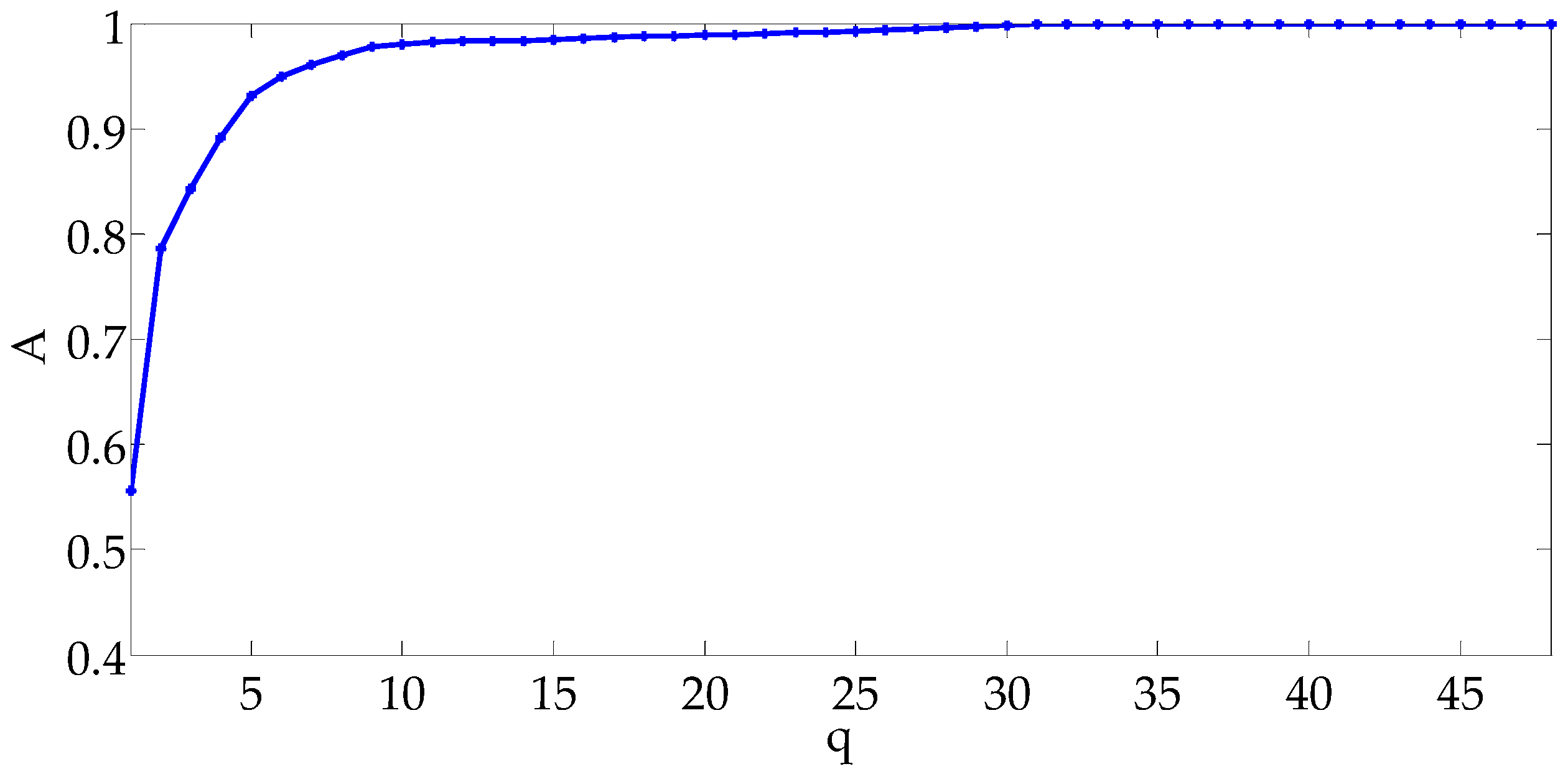
3.2.2. Determination of the Dimensionality of the Characteristic Information Matrix

The dimensionality of the characteristic information matrix $\mathit{Y}$ has an important impact on the effectiveness of the method proposed in this paper. To determine the dimensionality, the sum of squares of singular values is defined to represent the information contained in the matrix. The amount of information contained in matrix $\mathit{X}\prime$ is defined as $F={\lambda }_1^2+{\lambda }_2^2+\cdots +{\lambda }_n{}^2$; the amount of information contained in matrix $\mathit{Y}$ after dimensionality reduction is $F_1={\lambda }_1^2+{\lambda }_2^2+\cdots +{\lambda }_q{}^2$. The ratio of the characteristic information matrix $\mathit{Y}$ to the amount of information of the original matrix is $A=\frac{F_1}{F}$. In this research, a large number of experiments show that when $A>0.9$, the characteristic information matrix $\mathit{Y}$ can effectively express the information contained by the matrix $\mathit{X}\prime$. The value of $q$ is the dimensionality of the characteristic information matrix $\mathit{Y}$.

3.2.3. Solving the Assignment Matrix $\mathit{U}$

When solving $\mathit{U}$, Equation (11) can be simplified to

$$P(\mathit{U},\mathit{Z})={\displaystyle \sum _{p=1}^k{\displaystyle \sum _{i=1}^m{u}_{ip}{\displaystyle \sum _{j=1}^{q}w{\prime }_j{(y_{ij}-z_{pj})}^2}}}$$

(13)

The target function $P(\mathit{U},\mathit{Z})$ can be minimized if and only if

$$u_{ip}=\{\begin{array}{l}1,if {\displaystyle \sum _{j=1}^{q}w{\prime }_j{(y_{ij}-z_{pj})}^2\le {\displaystyle \sum _{j=1}^{q}w{\prime }_j{(y_{ij}-z_{p^{\prime }j})}^2}}\\ 0,otherwise\end{array}$$

(14)

where $u_{ip}=1$ denotes that the $i$th load curve is assigned to the $p$th class. Therefore, we can find the assignment matrix $\mathit{U}$. See [15] for specific demonstration details.

3.2.4. Solving the Clustering Center Matrix $\mathit{Z}$

Assuming that the assignment matrix $\mathit{U}$ obtained in Section 3.2.3 is fixed, the target function $P(\mathit{U},\mathit{Z})$can be minimized if and only if

$$z_{pj}=\frac{(1+\eta ){\displaystyle \sum _{i=1}^m{u}_{ip}{y}_{ij}-\eta {\displaystyle \sum _{i=1}^m{y}_{ij}}}}{(1+\eta ){\displaystyle \sum _{i=1}^m{u}_{ip}}-\eta m}$$

(15)

where $z_{pj}$ denotes the coordinate value of the $j$th dimension of the $p$th clustering center. Therefore, we can get the clustering center matrix $\mathit{Z}$. See [18,19] for a specific demonstration process.

The algorithm process is shown in Figure 2. The characteristic information matrix $\mathit{Y}$ and weight matrix $\mathit{W}\prime$ are obtained by the SVD of matrix $\mathit{X}\prime$. Then, the object assignment matrix $\mathit{U}$ and clustering center $\mathit{Z}$ are iteratively solved by Equations (14) and (15). Iteration is repeated until the value of target function (11) is no longer decreasing.

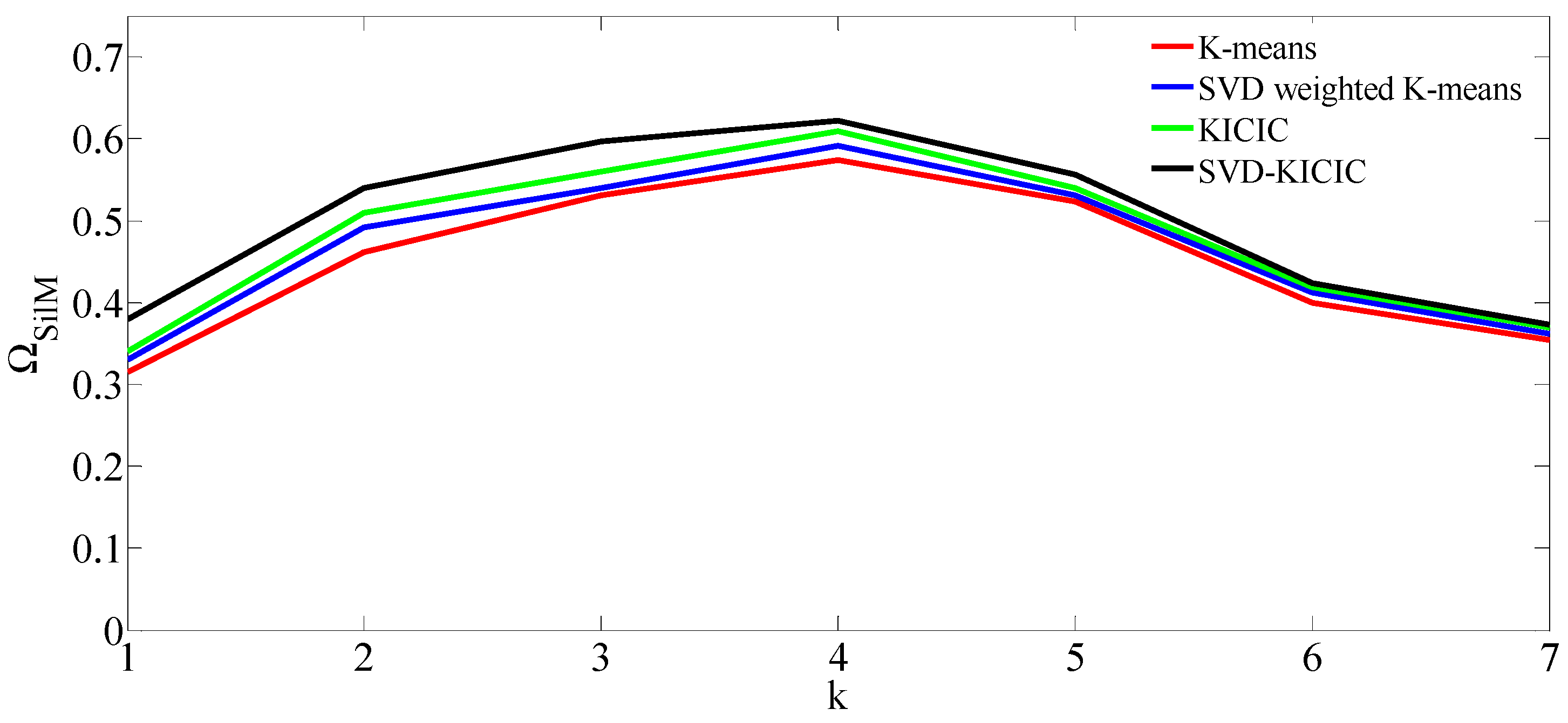
3.3. Clustering Effectiveness Indicator

The clustering effectiveness test is a process that assesses the clustering quality to determine the optimal clustering data set [20,21,22].

We assume that $m$ load curves are divided into $k$ classes. The Silhouette indicator ${\mathrm{\Omega }}_{Sil}$ of the $i$th sample in the $p$th class is defined as follows:

$${\mathrm{\Omega }}_{Sil}(i)=\frac{d_a(i)-d_b(i)}{\max (d_a(i),d_b(i))}$$

(16)

The overall clustering quality could be assessed by the mean value of Silhouette indicator ${\mathrm{\Omega }}_{SilM}$ of all load curves. A greater value denotes higher clustering quality. The clustering number $p$, corresponding to the maximum value of ${\mathrm{\Omega }}_{SilM}$, is used as the optimal clustering number.

The computational expression of ${\mathrm{\Omega }}_{SilM}$ is characterized by

$${\mathrm{\Omega }}_{SilM}=\frac{1}{m}{\displaystyle \sum _{i=1}^m{\mathrm{\Omega }}_{sil}}(i)$$

(17)

At the same time, the clustering results are assessed with the Davies–Bouldin index (DBI). DBI refers to the maximum value of the ratio of the sum of the average values of the intra-class distance of any two classes to the distance of their two clustering centers. A smaller value represents a better clustering result. The computational method is defined as follows:

$$I_{DB}=\frac{1}{k}{\displaystyle \sum _{a=1}^k\underset{a\ne b}{\max }(\frac{{\overline{C}}_a+{\overline{C}}_b}{M_{ab}})}$$

(18)

where $I_{DB}$ is the numerical value derived from DBI, ${\overline{C}}_a$ and ${\overline{C}}_b$ are the mean values of the sum of the distance from the two class samples to their clustering centers and $M_{ij}$ is the distance between the two clustering centers.

4. Analysis of Examples

The examples in this paper were realized on a PC configured with Inter(R) Core(TM) i5-8300H CPU 2.50 GHz, RAM 16 GB. The operating system used was Windows 10. To verify the accuracy and efficiency of the method proposed in this paper, the K-means algorithm, SVD-weighted K-means algorithm, KICIC algorithm, and SVD-KICIC algorithm were used to independently study the actual load curves of a certain city and the results, of the four algorithms are compared and analyzed.

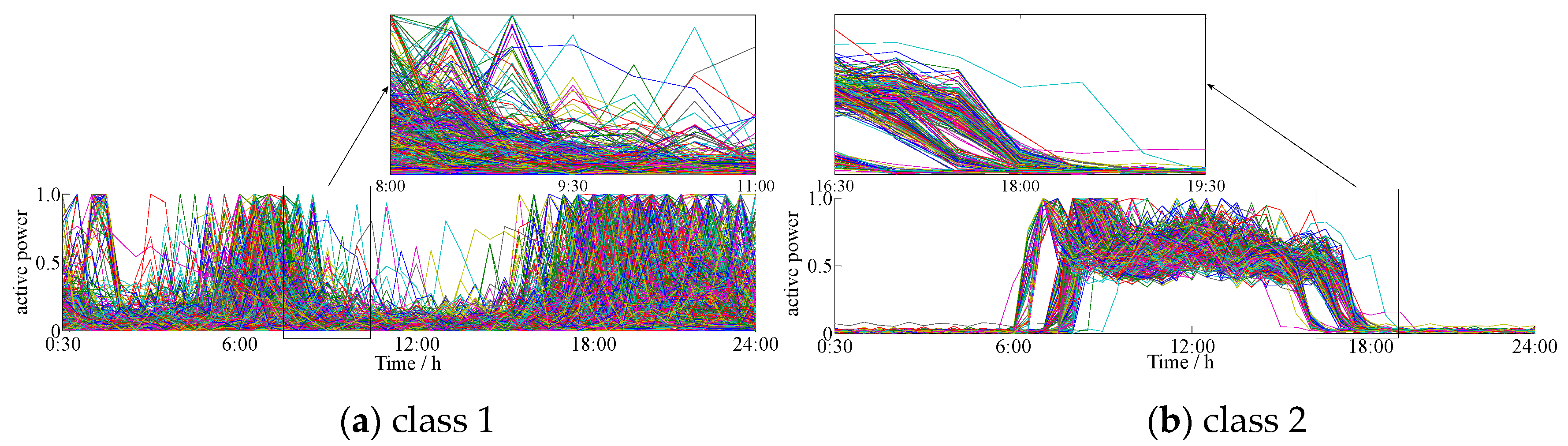
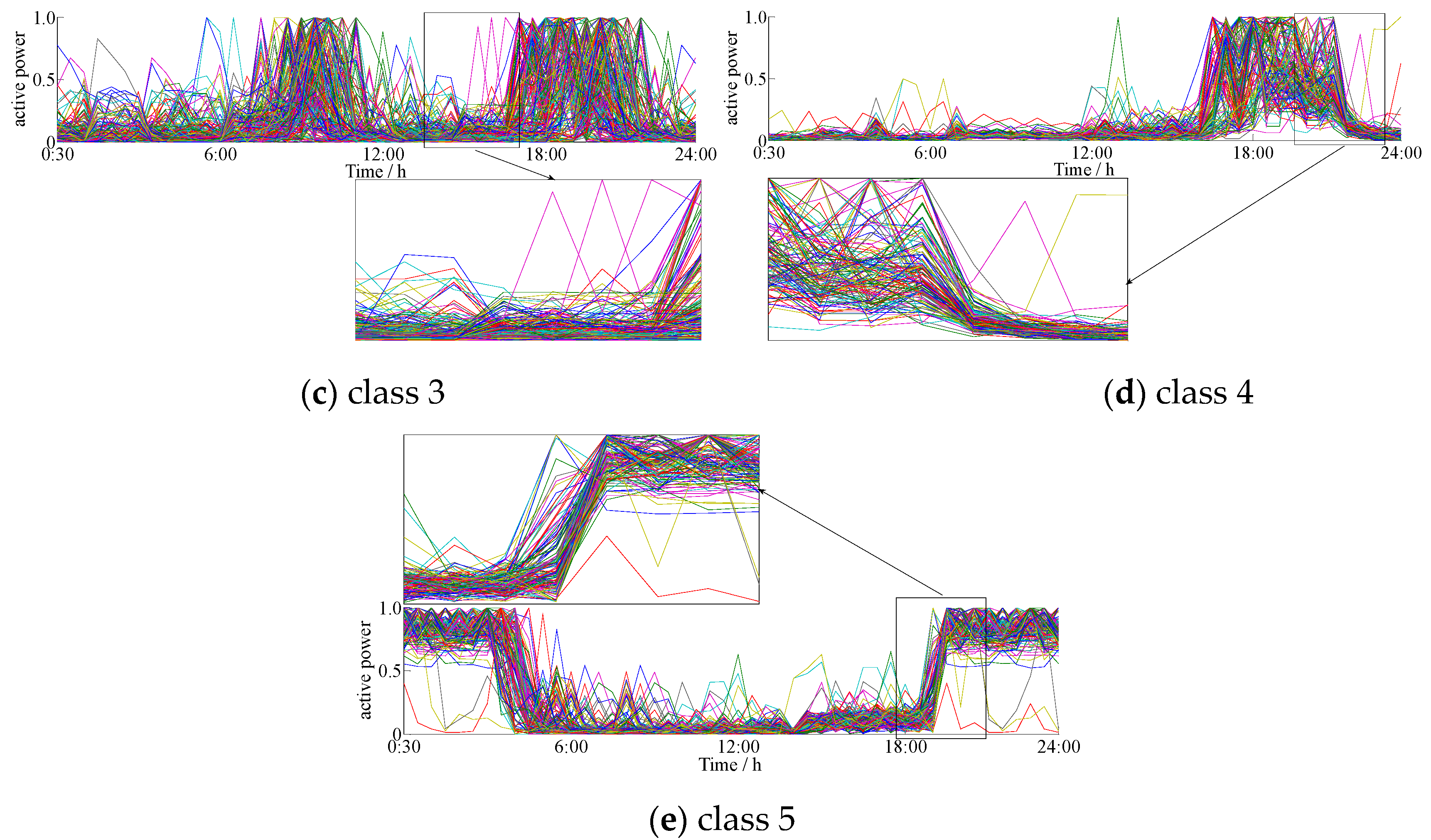
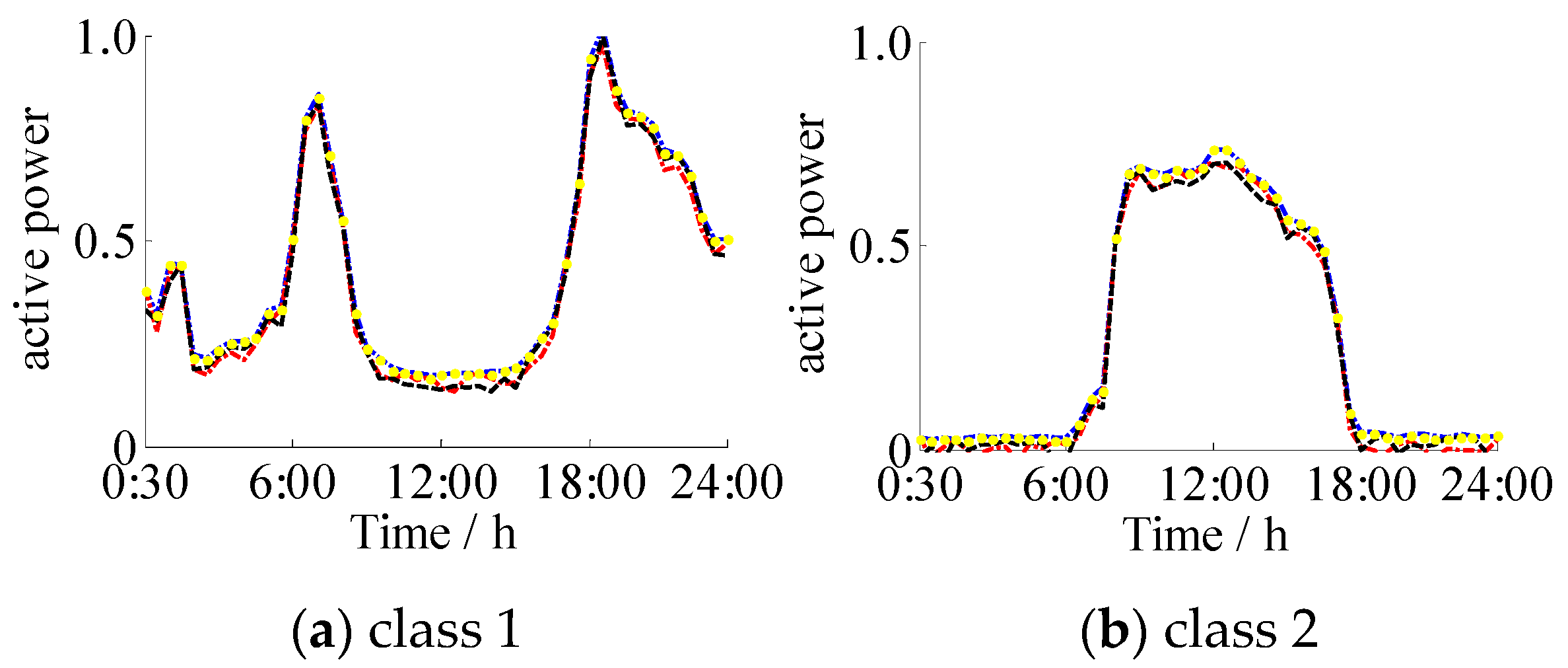
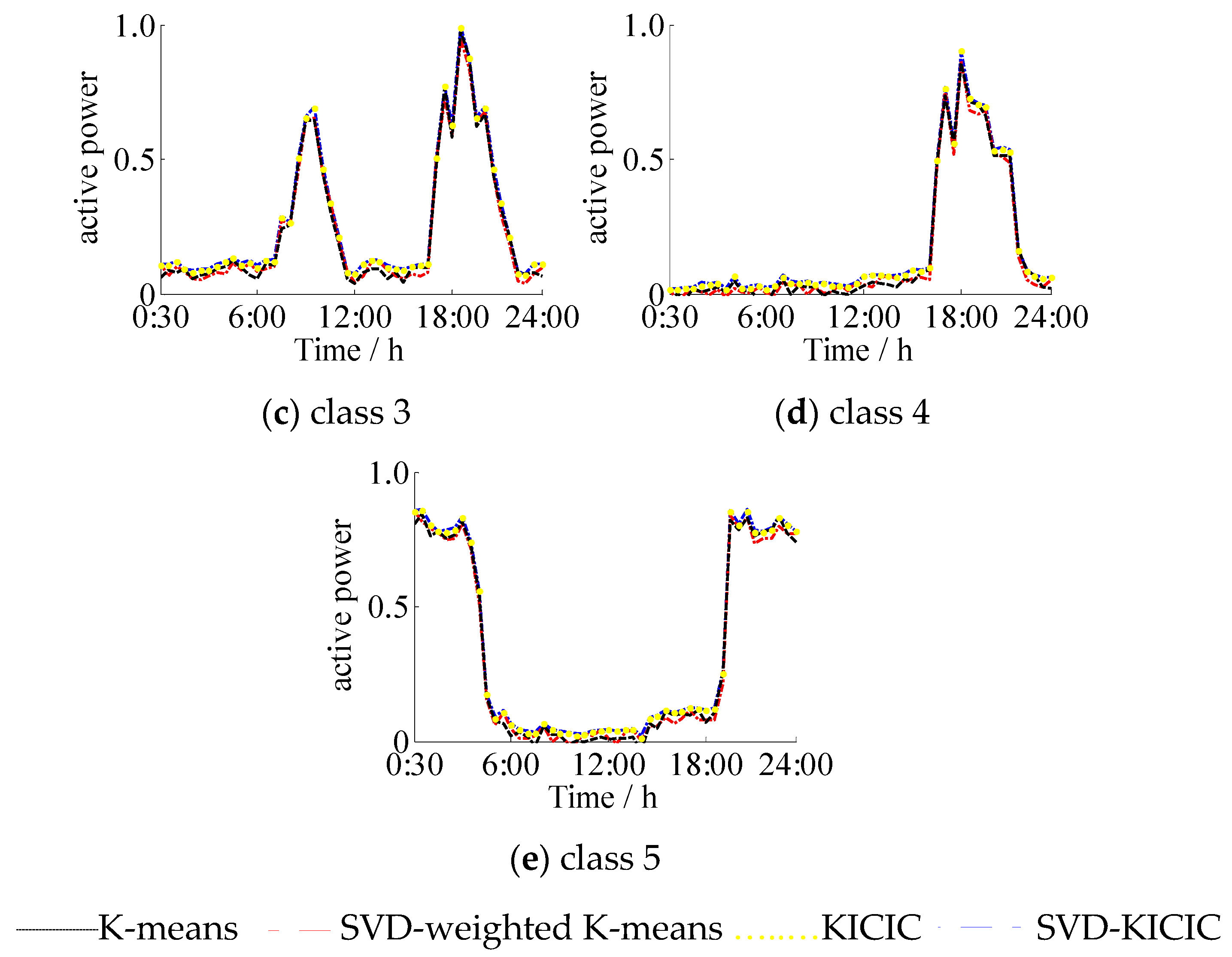
4.1. Clustering of Actual Daily Load Curves

The experimental data in this paper are derived from the data of 5263 measured daily load curves of a certain city. The sampling interval was 30 min, and each load curve had 48 sampling points. Because some data were missing or abnormal after data preprocessing, 5158 daily load curves were obtained, forming an initial matrix of 5158 × 48 orders.

After performing an exhaustive number of simulations, the clustering result with the highest accuracy was associated with the parameter $\eta$ = 0.07.

Singular value decomposition was performed for the matrix $\mathit{X}\prime$ to obtain a characteristic value matrix (48 $\times$ 48). As shown in Figure 3, as the dimension of the feature information matrix increases, the information ratio of the matrix $\mathit{Y}$ gradually increases at a lower rate. As shown in Figure 3, when the dimension of the characteristic information matrix is 5, the ratio of information is $A=\frac{F_1}{F}\ge 0.9$. Thus, matrix $\mathit{X}\prime$ is expressed as a 5158 $\times$ 5 matrix $\mathit{Y}$. The weight vector corresponding to the five [column] dimensions is $\mathit{W}\prime =\left[0.542,0.225,0.118,0.096,0.019\right]$.

The traditional K-means clustering, SVD-weighted K-means clustering algorithm, KICIC algorithm, and SVD-KICIC clustering algorithm were compared to perform a clustering analysis of the load data. The results are shown in Figure 4. In the case of setting different numbers of clusters, the validity test demonstrated that when the number of clusters was 5, the average values of the silhouette of the four clustering algorithms were all maximized. Therefore, we selected $\mathrm{k}=5$ as the fixed number of clusters.

The clustering result based on our clustering algorithm in this paper is shown in Figure 5. The numbers of various load curves were 1582, 1038, 1269, 845, and 424. The numbers of various load curves corresponding to the KICIC algorithm were 1618, 1022, 1237, 829, and 452. The numbers of various load curves of the SVD-weighted K-means clustering algorithm were 1650, 1015, 1217, 829, and 447. The numbers of various load curves of the traditional K-means clustering algorithm were 1691, 1026, 1258, 807, and 376. The clustering results are shown in Figure 5, and detail a number of load curves for a narrow time period as an example to make different load curves visible.

Figure 6 shows that the four clustering algorithms extracted five typical load curves with similar shapes to the load curve. There were four types: double peak, flat peak, single peak, and avoided peak. Class 1 was at the peak of electricity consumption at 8:00 and 19:00, which is typically household electricity, and Class 2 was at the peak of electricity consumption from 6:00 to 18:00, which is typically commercial electricity. Class 3 and 1 were both the double peak load types, the difference being that that Class 3 used less electricity than Class 1 from 23:00 to 6:00 the next morning. Additionally, Class 3 used electricity for small industries, and the electricity consumption time was more regular. Classes 1 and 3 were more likely to be misclassified. The clustering centers obtained by the SVD-KICIC algorithm and the KICIC algorithm were basically consistent. The clustering centers obtained by the K-means algorithm and the SVD-weighted K-means algorithm were relatively close, but the former two were partially different from the latter two in the clustering centers. This is because the SVD-KICIC algorithm and KICIC algorithm minimize the intra-class distance while maximizing the inter-class distance, making the classification results more accurate. Class 4 had the lower power consumption throughout the day but showed increased power consumption at night, which was a typical night load. Class 5 was the peak avoidance load. The clustering results reflect the five actual power load conditions and demonstrate the reliability of the SVD-KICIC algorithm.

Based on a comparative analysis of the average values of the clustering indexes obtained from 50 tests listed in

Table 1. Clustering property comparison between four methods.

Algorithm	Best k	${\mathrm{\Omega }}_{\mathit{s}\mathit{i}\mathit{l}\mathit{M}}$	DBI	Running Time/s
K-means	5	0.574	1.283	61.32
SVD-weighted K-means	5	0.591	1.206	24.71
KICIC	5	0.609	1.127	45.83
SVD-KICIC	5	0.622	1.007	19.35

, the SVD-KICIC algorithm can achieve better clustering quality when clustering the load curves. The proposed algorithm fully considered the intra-class and inter-class distance, thus making the intra-class distance of the load smallest and the inter-class distance the largest. The clustering center and the non-class samples were far away from each other, which reduced the impact of the non-class samples on the clustering accuracy and accelerated the clustering iteration process. Therefore, our algorithm runs faster than the traditional K-means algorithm, SVD-weighted clustering algorithm, and KICIC algorithm.

In order to further verify the stability of the algorithm, the standard deviation of the number of various load curves in 10 experiments was compared and shown in Figure 7. It can be seen that the mean value of standard deviation of the SVD-KICIC algorithm was the smallest, and the stability of this algorithm was better.

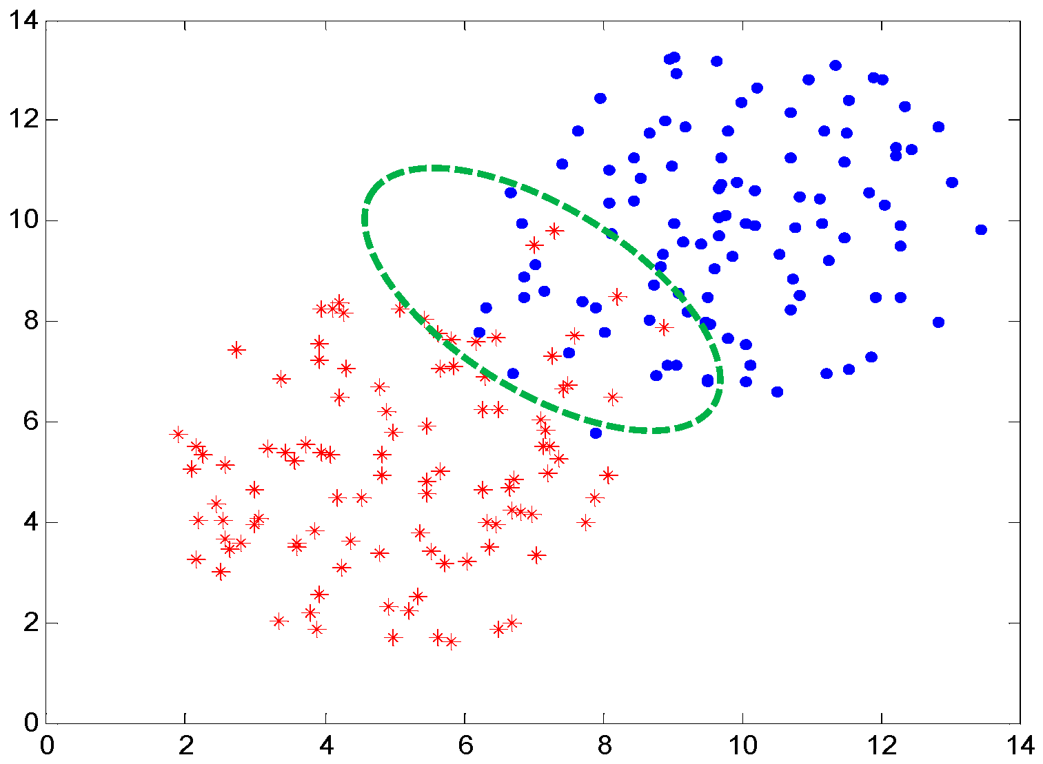
4.2. Simulation Examples

To verify the anti-interference ability and robustness of our algorithm, 5000 simulated load curves with known clustering results were selected and the distribution of the curves was randomly disrupted to perform clustering again. The results contained eight classes of typical load curves with different shapes, each comprising 625 load curves. Noise interference of different degrees within the interval of 5~40% was added to each sampling point of the simulated load curve to produce eight sets of simulated data. The step size 5% was chosen to effectively show the changing trend of the clustering results of the SVD-KICIC and K-means algorithms, so as to compare the clustering performance of the two algorithms. The load data were processed through the proposed algorithm. Simulation of 5000 typical load curves with $r=30\%$ is shown in Figure 8.

The effects of the noise of different degrees on the experimental results were tested and analyzed with the best cluster number, classification accuracy, and the Silhouette index mean.

Table 2. Comparison of robustness between two algorithms.

r/%	SVD-KICIC			K-means
	Best k	${\mathrm{\Omega }}_{\mathit{s}\mathit{i}\mathit{l}\mathit{M}}$	Acc/%	Best k	${\mathrm{\Omega }}_{\mathit{s}\mathit{i}\mathit{l}\mathit{M}}$	Acc/%
5	8	0.9516	100	8	0.9516	100
10	8	0.9233	100	8	0.9233	100
15	8	0.9085	100	8	0.8536	94.30
20	8	0.8860	100	8	0.8033	91.16
25	8	0.8649	100	7	0.7294	89.56
30	8	0.8327	99.85	7	0.6697	88.34
35	7	0.7638	90.63	7	0.6185	80.16
40	7	0.6079	78.41	6	0.5839	69.83

shows the results of the comparison between the SVD-KICIC algorithm and the traditional K-means algorithm in terms of clustering load curves under various noise interferences.

Based on the comparative analysis of the average value of the clustering indexes obtained from the 50 tests in Table 2, we find that, for the two algorithms, with an increase in the degree of noise interference, the optimal number of clusters deviate. The mean value of Silhouette indexes and classification accuracy show a decreasing trend, indicating that three indexes can be used to test the robustness of the algorithm.

When the noise ratio is between 5% and 20%, the optimal number of clusters for both algorithms is 8, and the classification accuracy is equal to or very close to 100%. When the noise ratio is between 25% and 30%, the optimal clustering number of the SVD-KICIC algorithm is always 8, the mean of the Silhouette is greater than 0.85, and the classification accuracy is equal to or very close to 100%. However, the optimal clustering number of the traditional K-means algorithm are changed to 7, and the clustering accuracy and Silhouette mean greatly reduce. When the noise ratio reaches 35~40%, the optimal clustering number of the two types of algorithms is not 8, and the classification accuracy and Silhouette mean of the SVD-KICIC algorithm decrease somewhat, but the fluctuation is small. Therefore, the SVD-KICIC algorithm is more robust than the traditional K-means algorithm.

5. Conclusions

In this work, we propose a clustering method of daily load curves based on SVD-KICIC by combining the advantages of the SVD dimensionality reduction technique and the maximized inter-class distance of KICIC. This method uses an SVD dimensionality reduction technique to extract the effective characteristics of load data and greatly reduce the data dimension; it also uses the singular value to determine the weight coefficient of KICIC and reduce the number of iterative calculations. Compared with traditional K-means, SVD-weighted K-means, and KICIC clustering methods, the simulation studies show that the method can effectively use the intra- and inter-class distances of load data to improve clustering quality, computational efficiency, and robustness.

References

1. Lu, S.; Fang, H.; Wei, Y. Distributed Clustering Algorithm for Energy Efficiency and Load-Balance in Large-Scale Multi-Agent Systems. J. Syst. Complex. 2018, 31, 234–243. [Google Scholar] [CrossRef]
2. Xu, X.; Chen, W.; Sun, Y. Over-sampling algorithm for imbalanced data classification. J. Syst. Eng. Electron. 2019, 30, 1182–1191. [Google Scholar] [CrossRef]
3. Qiang, C.; Xiuli, W.; Weizhou, W. Stagger peak electricity price for heavy energy-consuming enterprises considering improvement of wind power accommodation. Power Syst. Technol. 2015, 39, 946–952. [Google Scholar]
4. Lin, R.; Wu, B.; Su, Y. An Adaptive Weighted Pearson Similarity Measurement Method for Load Curve Clustering. Energies 2018, 11, 2466. [Google Scholar] [CrossRef] [Green Version]
5. Zhang, T.; Gu, M. Overview of Electricity Customer Load Pattern Extraction Technology and Its Application. Power Syst. Technol. 2016, 40, 804–811. [Google Scholar]
6. Bu, F.; Chen, J.; Zhang, Q.; Tian, S.; Ding, J. A controllable and refined recognition method for load patterns based on two-layer iterative clustering analysis. Power Syst. Technol. 2018, 42, 903–913. [Google Scholar]
7. Kim, N.; Park, S.; Lee, J.; Choi, J.K. Load Profile Extraction by Mean-Shift Clustering with Sample Pearson Correlation Coefficient Distance. Energies 2018, 11, 2397. [Google Scholar] [CrossRef] [Green Version]
8. Chicco, G.; Napoli, R.; Piglione, F. Comparisons among clustering techniques for electricity customer classification. IEEE Trans. Power Syst. 2006, 21, 933–940. [Google Scholar] [CrossRef]
9. Koivisto, M.; Heine, P.; Mellin, I.; Lehtonen, M. Clustering of connection point and load modeling in distribution systems. IEEE Trans. Power Syst. 2013, 28, 1255–1265. [Google Scholar] [CrossRef]
10. Zhang, M.; Li, L.; Yang, X.; Sun, G.; Cai, Y. A Load Classification Method Based on Gaussian Mixture Model Clustering and Multi-dimensional Scaling Analysis. Power Syst. Technol. 2019. [Google Scholar] [CrossRef]
11. Bin, Z.; Chijie, Z.; Jun, H.; Shuiming, C.H.; Mingming, Z.H.; Ke, W.; Rong, Z. Ensemble clustering algorithm combined with dimension reduction techniques for power load profiles. Proc. CSEE 2015, 35, 3741–3749. [Google Scholar]
12. Ye, C.; Hao, W.; Junyi, S. Application of singular value decomposition algorithm to dimension-reduced clustering analysis of daily load profiles. Autom. Electr. Power Syst. 2018, 42, 105–111. [Google Scholar]
13. Liu, S.; Li, L.; Wu, H.; Sun, W.; Fu, X.; Ye, C.; Huang, M. Cluster analysis of daily load profiles using load pattern indexes to reduce dimensions. Power Syst. Technol. 2016, 40, 797–803. [Google Scholar]
14. Deng, Z.; Choi, K.S.; Chung, F.L.; Wang, S. Enhanced soft subspace clustering integrating within-cluster and between-cluster information. Pattern Recognit. 2010, 43, 767–781. [Google Scholar] [CrossRef]
15. Huang, X.; Wang, C.; Xiong, L.; Zeng, H. A Weighting k-Means Clustering Approach by Integrating Intra-cluster and Inter-cluster Distances. Chin. J. Comput. 2019, 42, 2836–2848. [Google Scholar]
16. Golub, G.; Loan, C. Matrix Computation; Johns Hopkins University Press: Baltimore, MD, USA, 1996. [Google Scholar]
17. Zhang, J.; Xiong, G.; Meng, K. An improved probabilistic load flow simulation method considering correlated stochastic variables. Int. J. Electr. Power Energy Syst. 2019, 111, 260–268. [Google Scholar] [CrossRef]
18. Bezdek, J.C. A convergence theorem for the fuzzy ISODATA clustering algorithms. IEEE Trans. Pattern Anal. Mach. Intell. 1980, 1, 1–8. [Google Scholar] [CrossRef]
19. Selim, S.Z.; Ismail, M.A. K-means-type algorithms: A generalized convergence theorem and characterization of local optimality. IEEE Trans. Pattern Anal. Mach. Intell. 1984, 6, 81–87. [Google Scholar] [CrossRef]
20. Al-Otaibi, R.; Jin, N.; Wilcox, T.; Flach, T. Feature Construction and Calibration for Clustering Daily Load Curves from Smart-Meter Data. IEEE Trans. Ind. Inf. 2016, 12, 645–654. [Google Scholar] [CrossRef] [Green Version]
21. Li, Z.; Yuan, W.; Ren, C.; Huang, C.; Dong, X. Approximate computing method based on cross-layer dynamic precision scaling for the k-means. J. Xidian Univ. 2020, 47, 1–8. [Google Scholar]
22. Liu, Y.; Liu, Y.; Xu, L. High-performance back propagation neural network algorithm for mass load data classification. Autom. Electr. Power Syst. 2018, 42, 131–140. [Google Scholar]
Figure 1. Fuzzy boundary samples.
Energies 13 04476 g001
Figure 2. Clustering flow chart based on SVD-KICIC algorithm.
Energies 13 04476 g002
Figure 3. Proportion of information corresponding to dimensionality number.
Energies 13 04476 g003
Figure 4. Determining the best clustering number based on validity index.
Energies 13 04476 g004
Figure 5. Clustering results of load curves based on the SVD-KICIC algorithm.
Energies 13 04476 g005aEnergies 13 04476 g005b
Figure 6. Comparison of typical load profiles between four algorithms.
Energies 13 04476 g006aEnergies 13 04476 g006b
Figure 7. Comparison of stability between four algorithms.
Energies 13 04476 g007
Figure 8. Simulation of 5000 typical load curves (r = 30%).
Energies 13 04476 g008aEnergies 13 04476 g008b