Abstract
Renewables should become more continuously available, reliable and cost-efficient to manage the challenges caused by the energy transition. Thus, analytic and numerical investigations for the layout of a pilot plant of a concept called Fluidisation-Based Particle Thermal Energy Storage (FP-TES)—a highly flexible, short- to long-term fluidised bed regenerative heat storage utilising a pressure gradient for hot powder transport, and thus enabling minimal losses, high energy densities, compact construction and countercurrent heat exchange—are presented in this article. Such devices in decentralised set-up—being included in energy- and especially heat-intensive industries, storing latent or sensible heat or power-to-heat to minimise losses and compensate fluctuations—can help to achieve the above-stated goals. Part I of this article is focused on geometrical and fluidic design via numerical investigations utilising Computational Particle Fluid Dynamics (CPFD). In the process a controlled transient simulation method called co-simulation of FP-TES is developed forming the basis for test bench design and execution of further co-simulation. Within this process an advanced design of rotational symmetric hoppers with additional baffles in the heat exchanger (HEX) and internal pipes to stabilise the particle mass flow is developed. Moreover, a contribution bulk heat conductivity is presented to demonstrate low thermal losses and limited needs for thermal insulation by taking into account the thermal insulation of the outer layer of the hopper.
1. Introduction
In the course of the energy transition, the European electrical energy industry has to cope with increasing shares of volatile energy [1]. The basic problem concerning wind and solar power is temporal unreliability and limited predictability leading to a demand of flexible storage technologies in order to guarantee a stable power grid [2]. Existing storage technologies and capacities are pushed to their limits. At the TU Wien Institute for Energy Systems and Thermodynamics (IET) a novel storage technology, the Fluidisation-Based Particle Thermal Energy Storage (FP-TES), is developed and tested. The FP-TES concept is very flexible in application and can be utilised as a power to heat to power (P2H2P) system as well as for heat recovery and storage in general. More exotic applications as a reactor for bulk materials in the process industry or countercurrent heater or roaster in the food industries lie in the future. The concept is a further development of the SandTES project [3], another TES system designed by the TU Wien IET. Contextual knowledge on this project can be found in [4,5,6].
Different process designs using fluidised bed heat exchanger (HEX) and particle TES are already presented in context with concentrating solar power applications [7,8,9]. In [10], also the design of the hopper for storing the particles and its insulation are examined.
A significant advantage of FP-TES compared to other particle-based storage systems, and therefore also the SandTES system, is a total substitution of mechanical transport devices, limiting operating temperatures and lifetime. This enables high cost efficiency and low thermal losses. An advanced fluidisation technology allowing powder transport via pressure gradients across communicating fluidised beds has been developed for this purpose. Therefore, the FP-TES enables countercurrent flow in the HEX, which otherwise has to be managed by a cascade of a couple of HEX [11]. The fluidic basic design of this novel approach based on numerical investigations with the CPFD software Barracuda is presented in this article. The software is already successfully applied in simulations of bubbling [12,13] and circulating fluidised beds [14,15,16]. The main goal of the presented investigation is to develop a functional layout of the novel TES system and prove the applicability of the concept. The essential targets to be achieved in this work are listed below.
- A validation of the FP-TES transport principle utilising comparably fast simulations with simplified geometries—ideally powder transport via plug flow—aiming for efficient countercurrent heat exchange. Subsequent determination of an advanced geometry for a test bench aimed for minimum dead storage volume and minimum foot print.
- The improvement of fluidic design advanced geometry by stabilising local pressure losses and related particulate mass flows aiming for maximum flexibility and stability during operation.
- The validation of mass flow control of the advanced geometry via co-simulation of FP-TES with a controller code and the evaluation of possible minimum and maximum stable mass fluxes.
Related challenges are represented mainly by the transport into and out of completely emptying hoppers and the stable operation and control of powder mass flows in a countercurrent HEX. Especially, the development of a transient co-simulation approach to deal with changing boundary conditions is a complex challenge. In the literature some approaches for different fields of application are reported [17,18,19], but a solution for this unique problem is not presented so far. Subsequently, an optimised geometry for a cold test rig, working with 800 kg quartz sand, is developed. Its behaviour as well as particle mass flows and pressure drops were predicted by simulations performed with Barracuda in the masters thesis of the first author [20], on which this paper is based. The results of experimental investigations performed with the test rig are presented and compared to the numerical simulations in Part II of this article [21]. The first paper showing the results of preliminary simulations and validation by means of experiments is already published [22]. In [21], an energetic consideration of a real industrial application is performed and major losses as well as auxiliary energy demand are addressed, revealing an overall energetic efficiency between 0.9 and 0.98 depending on the working medium and the charging and discharging conditions. Further information on fluidised bed technology [23,24] and possible storage materials [25,26] can be found in the literature.
2. Basic Concept of FP-TES
FP-TES is meant as an ordinary countercurrent flow regenerative HEX with the more specific features of a short- to mid-term heat storage ability yielding minimal losses and high energy density [3]. This is to be achieved by storing heat in low-cost powders (like quartz sand or corundum powder) and transporting those powders through a HEX between a hot and a cold particle storage device. The HEX contains a tube bundle for heat exchange with a sensible process fluid (like thermal oil or molten salt), which is moving in the opposite direction of the working medium. One of the great advantages of countercurrent flow is the possibility of extracting a higher proportion of the heat content of the heating fluid compared to cocurrent flow. A possible tube bundle geometry for the FP-TES is presented in [21] or in [5] for a longer HEX. In case of electrical energy input, the HEX additionally contains electrical heating rods. To implement a countercurrent regime in the HEX, the powder is fluidised with air and transported by applying a pressure gradient. The main capacity limiting factor for this technology is expected to be the maximum stable height of the fluidised bed in the storage hoppers and also a difficulty of fully emptying them, at least in the early stage showed in Figure 1.
Figure 1.
Early conceptual sketch of Fluidisation-Based Particle Thermal Energy Storage (FP-TES) [22].
Figure 1 depicts the essential process layout and the very crux of the matter: The chambers seen in Figure 1 are geometrically and procedurally separated by baffles reaching below the levels of fluidised powder. Those separated chambers, which include the hoppers, enable the build up of a pressure gradient by simply throttling the fluidising air entering from below at the top sections of those chambers, permitting a potentially very compact design. Throttling as well as flow regulation of the fluidisation air is applied via control valves. The stated chambers can be seen as communicating fluidised beds in an analogy to communicating containers with liquids, which behave similarly in many regards. The dark grey areas show fixed bed regimes, while the fluidised zones are highlighted by dots.
3. Numerical Simulation Approach
3.1. Simulation Set-Up
In the process of the procedural and fluidic layout of FP-TES several key issues occurred. Most of those require a numerically based approach by utilisation of the powerful CPFD software—Barracuda (version 16.0.8). Processes taking place in the fluidised domain inside FP-TES are highly complex and could not be addressed with an analytic or known empirical approach. This is caused by the fact that hundreds of billions of particles are being lifted, dragged and colliding with walls and each other at the same time. However, those processes need to be taken into account to validate essential working principles and allow raw dimensioning of necessary fluidisation grades (FG), pressure gradients and manageable particle mass fluxes . Another aspect is the continuous pressure variations above the distributor floors, needed to layout the floors’ pressure losses enabling homogeneous air distribution across those surfaces. Subsequent bench experiments would prove that Barracuda is a genuine choice as simulation software to aid the layout of FP-TES. This is presented in Part II of this article. The mayor assumptions for the numerical model can be summarised as follows.
- Adiabatic wall treatment
- Buoyancy effects are taken into account
- Empiric fixed bed porosity is taken into account
- Gas to wall, particle to wall and particle to particle friction and impacts are taken into account
- Gravitation is taken into account
- Isothermal simulation
- Sphericity of particles is taken into account
- Wetness of air and bed materials are neglected
The calculation of particle and fluid phase in Barracuda can be thought of as two separate solvers communicating with each other regarding local boundary conditions (lift, drag, displacement, etc.). The fluid phase is described as continuum with a Eulerian coordinate grid, while the discrete particle phase benefits from a gridless Lagrangian formulation. The solver utilises a relaxation-to-the-mean term for damping of colliding particles [27]. It considers only the impact of a particle hit by other particles but not the other way round, [28]. Particle collisions are modelled with a normal stress function. Its spectral gradient is calculated on the Eulerian grid and then interpolated to discrete particles treated as a continuum—a momentum equation is solved for every particle. The Wen–Yu model is applied for definition of the fluid drag and resulting minimum fluidisation velocities () [29,30]. The Large Eddy Simulation (LES) method describes turbulence. Barracuda applies the Smagorinsky subgrid scale (SGS) model, based on the linear relationship between SGS shear stresses and resolved rates of strain tensors [31]. The advection term is discretised via partial donor cell differencing utilising a weighted average distribution [32]. The calculation would be too slow for large amounts of particles if they were not clustered to form so-called computational particles, which represent differing amounts of particles with (ideally) similar properties regarding material, density, size and temperature. The amount of particles in a computational particle primarily depends on local boundary conditions and the overall number of discrete particles in the modelled system. All numerical investigations featured in this paper are set up at constant temperature of 37 C and no heat exchange is taken into account, as the fluidic design and related behaviour of FP-TES are of essential interest considering the targets presented above. The value was chosen based on the boundary condition for a cold test rig in the laboratory, presented in Part II of the paper.
To enable comparably fast simulation results with the applied hardware for all presented simulations, no tube bundle is implemented into the HEX. However, introduction of a tube bundle in the HEX is expected to benefit and stabilise plug flow by reducing vertical and horizontal mixing in the particle flow. This should be taken into account considering the results presented in the following. The set-up for the CPFD simulations are summarised in Table 1.

Table 1.
Set-up for the CPFD.
The utilised bulk material is quartz sand with a density of ≈2650 kg/m. Additional applied parameters concerning the constant simulation temperature ; the bulk porosity , the minimum, mean, and maximum particle diameter ; the sphericity S; and the minimum fluidisation velocity can be found in Table 2.
Table 2.
Properties and working conditions for quartz sand.
Figure 2 shows the three CFPD simulation set-ups. In all cases, yellow areas represent pressure boundary conditions and red areas represent flow boundary conditions. At first a simplified geometry (Figure 2a) is used to validate the FP-TES basic working principle and a desirable flow regime in its HEX. The applied geometries allow a low grid resolution. It is not the goal of this model to calibrate mass flows or perform a quantitative approach of any kind. The only baffles installed in this geometry are the indispensable upper baffles separating chambers at differential pressure levels. Lower baffles are completely missing at this point. Figure 2b is still a simplified geometry but with upper and lower baffles and an improved hopper design, which should enable complete emptying based on gravitation. The advanced geometry presented in Figure 2c is an simulation model of the FP-TES rig aimed for more complex investigations. The geometry of the HEX is the same as developed with the simplified model (Figure 2b), but now the investigations focus on the hopper design and interaction of all parts with regard to the cold test rig in the laboratory. The numbers 1–5 represent independently pressurised chambers. The Roman numbers I–VII represent sintered floor and wall areas for an uniform air distribution. Consequently, an independent fluidisation of the pressurised chambers 1–5 is also possible. The cross-sectional area of the risers (chambers 1 and 5) connecting the HEX to the hoppers has been further reduced to save fluidisation air and reduce auxiliary power consumption.
Figure 2.
(a) First simplified FP-TES geometry, (b) improved simplified geometry and (c) advanced geometry of FP-TES for detailed simulations with yellow areas representing pressure boundary conditions and red areas representing flow boundary conditions.
The grid consisting of hexahedral elements has been created utilising Barracudas own meshing tool. The number of cells for all in Figure 2 presented cases are shown in Table 3.
Table 3.
Mesh size.
Furthermore, the dimensions of the advanced geometry model are chosen based on the requirements of a future test bench to enable scaling of experimental investigations. It features a HEX length of 1500 mm, a width of 250 mm and an unobstructed height of 129 mm. Considering the compressibility of the introduced air over the beds height, a wider bed demands less compressor power compared to a more narrow and deep bed for most bulk materials considered in context with FP-TES. The hoppers have a cylindrical height of m and a diameter of m each.
A future test bench or industrial application of FP-TES would need some minimum space between the large hoppers and the HEX for reasons of construction and assembly. The risers will have to reach higher compared to Figure 2b. In any case, further numerical investigations show that a fast fluidisation of the potential significant hopper height in such application is challenging. The introduced air at the bottom of the risers tends to take the path of the lowest resistance into the HEX instead of the hoppers. To ease and accelerate start-up, the fluidisation areas and are introduced.
Figure 3 shows the positions of 456 data points per hopper for logging of the porosity and the 25 pressure measurement points. The former are utilised for monitoring only, while the latter are utilised for monitoring and control of the more detailed numerical investigations. The driving pressure differences between the chambers 1–5 are dependent on the flow of fluidisation air from below and the throttling of the same air at the chambers exits, realised by pressure boundary conditions. The pressure difference between the HEX and the hoppers is responsible for the particle flow out of and into the hoppers. As in the pressure in the chambers of the HEX, the pressure in the hoppers is controlled by throttling the leaving air at the top of the hoppers. Indeed, the applied driving pressure differences are small compared to the hydrostatic pressure differences along the hoppers heights and the dynamic pressure losses in the risers and their connections to the HEX. In addition, FP-TES is very fast reacting—a benefit for versatile operations, but a challenge for control. Thus, the term of communicating fluidised beds in analogy to communicating containers of liquid is a useful aid for the imagination. The flux planes for logging of particle mass fluxes set in Barracuda are shown in Figure 4. In the following mass fluxes and flows will be designated with the indexes L, , and R referring to this figure.
Figure 3.
(a) Four-hundred-and-fifty-six data points per hopper for logging of the porosity and (b) 25 data points overall for the pressure p, as set up in Barracuda, [20].
Figure 4.
Flux planes for logging of particle mass fluxes, as set in Barracuda [20].
3.2. Co-Simulation Approach
To achieve control of FP-TES working pressure gradients and related particle mass flows during simulations, a novel co-simulation approach is established by application of a Matlab (version 2015) controller script (see Figure 5). It has the tasks of continuously reading and interpreting data from Barracuda simulations and specifications given by the user to again define needed input parameters determining the boundary conditions for a running Barracuda simulation. First, the controller reads and processes the data from Barracudas log files plotted for measurement dots and flux planes defined with the grid. The most important data are the fluid pressure p, the fluidised beds porosity and the particle mass flux . The script plots and prints are part of the acquired information to enable quality control by the user (p, and , where A is the cross section of the HEX or more generally a flux plane). Then, it calculates the minimum fluidisation velocity from particle and fluid parameters to translate the fluidisation grades (s) given by the user into air mass fluxes through FP-TES distributor floors. The distributor floors are set as so-called flow boundary conditions in Barracuda (at the bottom of each FP-TES chamber, see Figure 2). The next step is the calculation and setting of Barracudas pressure boundary conditions, meaning the controlled pressures at the top of each chamber including the hoppers. Those are derived from the desired pressure gradients set by the user, corrected with varying hopper pressure differences (due to varying fluidised bed levels in the hoppers read from the log files). In a test bench, both kinds of boundary conditions would have to be set by control valves. Finally, the controller writes the exact simulation time at the start of its execution to another log file to enable comparison of the current simulation time in Barracuda with the time of the last controller execution for co-simulation respectively simulated control of FP-TES. To enable real co-simulation, meaning actual simulated control of Barracuda by the Matlab controller based on above mentioned parameters set by the user, a Python script has been utilised. This script reads the current simulation time from a Barracuda log and compares it to the time of last execution written by the controller. If a certain time step (again given by the user) is exceeded it starts Matlab, executing the controller, again closes it and then initiates a new read-in of boundary conditions by Barracuda (green path Figure 5). To achieve a co-simulation, this process is repeated continuously. Based on the actuating time of valves in the experimental test rig, the time step for the controller is set to s for the presented numerical investigations. The influence of a slightly different timestep according to those boundary condition is tested leading to no significant difference in the results.
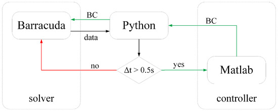
Figure 5.
Co-simulation approach to enable transient control of Barracuda [22] (BC refers to boundary conditions).
4. Numerical Investigation Results
4.1. Results of the Simulations with Simplified Geometries
To prove the FP-TES basic working principle simulations are carried out with the set-up presented in Figure 2a. The particle species distribution across the model is depicted in Figure 6. Light blue, green, yellow and red areas represent differently coloured species of the same bulk material which are used to evaluate the particle transport mechanism. The upper baffle lower edges are marked with a black line for better visibility.
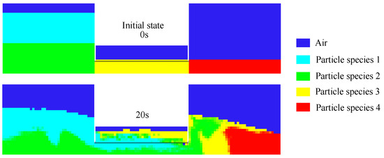
Figure 6.
Particle distribution shown by the mixing of four differently coloured particle species.
An initial distribution and one after 20 s of simulation time are shown. Dark blue areas hold no particles. It can be easily observed from Figure 6 that without additional upper baffles significant vertical (and it seems even some horizontal) mixing occurred. A black line has been added for a better visibility of this phenomenon. It is highly undesired in a fluidised bed HEX as it potentially reduces exegetic efficiency and has a negative impact on countercurrent heat exchange. Another more obvious disadvantage with this geometry is the impossibility of a satisfactory emptying of hoppers, meaning there would be a large dead volume of powder unable to take part in the process representing mere dead freight. However, obviously a basic functionality of FP-TES essential transport principle is confirmed by Barracuda. To address the issues with emptying and mixing, rotationally symmetric raised hoppers, more upper baffles and additional lower baffles were introduced in a second simplified model. In addition, the rotational symmetry of hoppers enables better stability under internal pressures due to process pressure gradients and powder loads. An ideal HEX regime for countercurrent heat exchange in a multiphase regime is a plug flow, meaning a constant velocity profile in each cross section with no vertical or back mixing, below and between baffle edges.
Figure 7 depicts simulation with the slightly improved geometry again utilising coloured powder species and boundary conditions equivalent to Figure 2b. Significantly improved mixing behaviour can be observed with the new HEX geometry, which also includes lower baffles. The baffle spacing is irregular to limit vertical flow oscillation. At this point of the investigation with a simplified model it is decided sufficient for the given application. The result can be described as an approximation of the desired plug flow. This behaviour is expected to be further improved with implementation of a horizontal tube bundle in a test rig or further simulations.
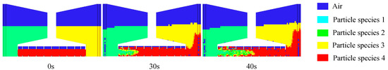
Figure 7.
Coloured particle species distributions at the times of 0, 30 and s, demonstrating approximate plug flow in the HEX.
Figure 8 shows particle mass flow normalised with its maximum and averaged over 200 s. Green areas represent unity while the blue areas represent zero. Averaged mass flows are shown in this figure to monitor if any noteworthy particle flow occurs in undesired regions above or below the main flow channel between the baffles edges. Some particle flow oscillation may be observed, but in a stable and controlled manner. HEX in- and outflow is more or less horizontally oriented. The sharp edges and vast thicknesses of the baffle plates are not desired but a side effect of Barracudas grid generator. It utilities the same grid for geometry and fluid calculation, again defining fineness of computational particle boundary conditions in the solver. This causes an impossibility of separation concerning the degree of detail in geometry and fluid calculation grid and consequentially forces the user to compose the geometrical grid as crude as possible with the desired degree of detail regarding results. This is due to the huge computational effort of CPFD. It is shown that applying larger number of baffles is redundant to the effect of the irregular spacing in therms of limiting vertical flow oscillation. Therefore, the advanced geometry is designed with regular HEX baffle spacing. Moreover, the lower HEX baffles are shorter compared to the upper baffles, to save space. The simulations with simplified geometries showed that bigger length does not add significant stability to plug flow. The space above the main flow channel has been increased to prohibit fast plugging of outlets and related difficulty of pressure gradient control. Therefore, the most important geometrical characteristics of the HEX are defined.
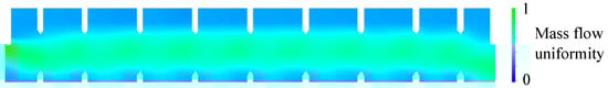
Figure 8.
Uniform particle mass flow along the HEX, averaged over 200 s.
4.2. Results of the Simulations with Advanced Geometries
As explained in the set-up chapter, the simulations with advanced geometry (Figure 2c) are aiming for more detailed investigations. The stabilisation of local pressure losses and related particulate mass flows targeting maximum flexibility and stability during operation had shown to be challenging. Additionally, validation of mass flow control for a future test bench via co-simulation of FP-TES with a controller code and the evaluation of possible minimum and maximum stable mass fluxes have been done.
The hydrostatic (vertical) pressure difference in a fluidised bed
with the particle density , the fluidisation air density , the bed porosity and the bed height h. Measurement of the average porosity along a beds height h poses a significant problem in practice. Thus, a test would need many pressure measurements along the particles flow path. The relation between hopper (and HEX) pressures needed to control the process in the numerical investigations and later on in bench experiments has been set up in [20] as
where and represent the pressures at the top of the storage hoppers measured by the uppermost pressure checkpoints depicted in Figure 3. Thus, or , respectively, are always to be set to the minimal pressure allowed to occur () in terms of calculating the other. and are the pressure drops in the respective hoppers fluidised beds obtained from respective pressure data points (Figure 3). They result almost exclusively from hydrostatic pressure differences, assuming stable fluidisation dynamic pressure losses are negligible. For the same reason, the pressure differences between the HEX segments result almost exclusively from throttling of air at their exits. Equation (2) presents the same pressure gradient in between HEX segments twice, though two different values could also be applied. This can be useful for a longer HEX in an industrial application, e.g., for transport around corners with comparably higher pressure loss.
and are the pressure differences between the left hoppers riser and the HEX and again from the HEX to the right hopper in this order. They cannot be modelled via Equation (1), as they do not result from hydrostatic pressure differences but from dynamic pressure losses due to sharp geometries, locally high velocities, introduction of fluidisation air and related bubbling. It seems they correlate with the effective particle mass flow along the HEX. In bench tests this mass flow is very difficult to determine as its measurement can only be accomplished by complex set-ups of scales or calibration of strain gauges The initial bed heights in the left hopper is set to m and, respectively, in the right hopper to m. In the following, a simple abbreviated form is used to define applied and working pressure differences . The actual superficial bed velocity is a multiple of . The fluidisation grade is defined via . The working pressure differences are defined from left to right via : || in Pa, referring to Equation (2) (e.g.,: : |2000 500 1000|). It should be kept in mind that both contain the above-stated equality term of Pa (positive on the left side, negative on the right side) and and are calculated from the data yielded by the pressure measurement points shown in Figure 3. The fluidisation grades are defined again ranging from left to right via : || referring to the Roman numbered fluidised floor areas in Figure 2c (e.g.,: : |12 10 6 6 6 10 12|, to are set to the same value).
The major challenge discovered by the advanced simulations of FP-TES is the influence of bubbling in the risers on the particle mass flow. Above a certain absolute bed height of ≈1.5 m, it becomes impossible to stabilise the fluidisation in the risers and therefore limits the maximum hopper bed levels. As the maximum hopper bed levels (in addition to their diameters) determine the maximum bulk storage capacity of the FP-TES, this is not acceptable. Excessive build-up of huge bubbles with bigger bed heights is demonstrated in Figure 9 by the horizontal particle flow velocity .
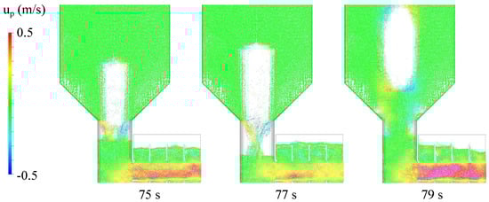
Figure 9.
A plot of the horizontal particle flow velocity (in m/s) demonstrates coalescence and disengagement of a large bubble and related particle mass flow fluctuation; : |1000 250 200|, : |23 10 10 10 10 10 11| [20].
Even with application of excessive high fluidisation grades (: |23 10 10 10 10 10 11|) no stable fluidisation of the hoppers is achieved. The central mechanism of several smaller bubbles or one large bubble being shaped in and just above the riser, and thus producing frequent short-term blockades for the flow at the base of the hopper, can be observed well. Stable outflow at the hoppers exit is blocked by uprising bubbles with irregular intervals. At some point the large bubble gives way and tears itself loose, puncturing the bed and making way for the out-flow again. The flow regime defining hopper out-flow as calculated by Barracuda, appears to be mass-flow. Typical regimes of hopper emptying flow can be found in the literature [33] and are depicted in Figure 10. Hopper outflow to persist during and immediately recover to full magnitude after a bubble tears loose (as shown in Figure 9) would not be possible with funnel flow. The centre of the funnel would still be blocked by the bubble. An error source would be the assumed sphericity set in the simulation. A mass-flow regime in the hopper would render fluidisation in the desired sense impossible, as the fluidised bed would be perpetually choked by powders rushing down from all sides. The resulting undesired fluidisation regime, which also can be observed in the experiments [21], is irregular formation of large bubbles charged with air until they develop enough lift to punctuate the bed, which itself immediately fills the space in a bubbles wake. Another theory explaining the occurrence of what seems like mass-flow would be the bubbles supportive effect on the powder layers above. This compressed and strutted powder volume might for once carry a significant portion of its weight by itself and is additionally lifted from below effectively reducing the bed level which represents a significant influence on the flow regime, as it defines the powder load compressing the lower layers of a bed. Obviously usual applications of hopper out-flow regimes would not necessarily incorporate a fluidisation through the same opening. Actually, assuming such fluidisation to be stable a stabilising impact on a forming funnel could be expected. However, the emptying mechanism needed for stable control and HEX particle fluxes for the FP-TES would be the funnel-flow. To ensure such flow regime at any hopper bed level and in any state of operation pipe-shaped hopper installations are tested in further numerical investigations.
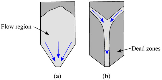
Figure 10.
Hopper emptying mechanisms: (a) mass flow and (b) funnel flow.
Figure 11 shows four different pipe geometries fixed in the hoppers centres. The first one is a simple pipe without any openings (1). The second one features rotationally symmetric circular ring openings (2). The third pipe shows several asymmetric horizontal openings along a part of the circumference (3) and the fourth a slit along its length.
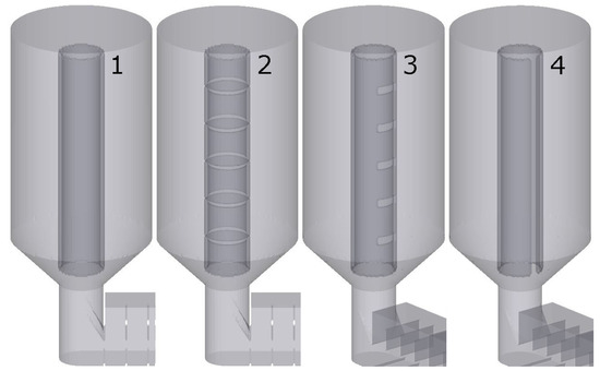
Figure 11.
Pipe geometries implemented into the hoppers [20].
Asymmetric openings should be directed away from the usual inflow during fluidisation, which is usually displaced outwards from the hoppers centre. Those pipes are being referred to as pipes 1–4 in the following. Fluidisation grades during start-up are set to : |14 13 0 0 0 13 14|. The pressure gradients are set to : |+1300 0 −1300|. During transport s are |12 10 6 6 6 10 12| and gradients are initialised to : |+1800 100 −800| at s. The set-up equipped with Pipe 1 can be flawlessly fluidised within 33 s, which may be expected due to apparent genuine containment and separation to the surrounding powder of the vertical fluidisation air mass flow. However, it is incapable of particle transport into a hopper with lower bed heights and related lower pressure loss in the surrounding powder, compared to the tube. Thus, the fluidisation air bypasses the pipe. The consequence is a collapse of fluidisation and impossibility of refluidisation which is depicted in Figure 12. The root cause is an impossibility of equalisation of tube respectively surrounding hopper bed levels with a closed tube. Unfortunately pipe 2 is found not sufficiently fluidisable after a futile start-up duration of 185 s. This has been tested at various s within reasonable boundaries. The issue is shown with Figure 13.
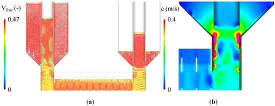
Figure 12.
Pipe 1 is bypassed and thus rendered incapable of transport after 74 s and , unitless (a); positive z-direction fluid velocity bypass, m/s (b) [20].
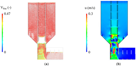
Figure 13.
Pipe 2 is plugged due to rotationally symmetric frictional locking after 185 s and , (a) unitless and (b) positive z-direction fluid velocity (m/s).
It is attributed to the powder contained in the tube above the bubble being compressed and thus effectively forming a plug due rotationally symmetric frictional locking with the surrounding bed and tube. The related fluidisation grades are : |15 13 0 0 0 10 12|. However, a dismissal of rotational tube symmetry should also disable rotationally symmetric frictional locking respectively offer a zone of less tightly compressed powder to the fluidisation air at all times.
Tube 3 finally is fluidised in 110 s after start-up and transport is accomplished. The equilibrium state at : |1300 0 −1300| is achieved for the first time with this set-up. The break-through of first bubbles and the flow of sand through the tubes orifices are shown in Figure 14. Collapse of the fluidisation in the right hopper at a low bed level is again attributed to the bypass of fluidisation air through the bed surrounding the pipe. Bed level equalisation with pipe 3 is obviously still not ideal. Nevertheless, this set-up reacts quite well to changes of pressure gradients and the controller manages more or less stable mass flow rates at control intervals of s. In addition it is observed that a gradient ( Pa) and subsequent transport directed from the left hopper to the HEX applied at just the right moment can significantly speed up start-up durations (≈−45%) by—it seems—creating space for the rising air respectively increasing of the to be fluidised packed bed. This may further improve the flexibility of FP-TES. As an answer to pipe 3’s insufficient level equalisation behaviour, pipe 4 is designed and implemented. Its vertical slot is directed away from inflow enables continuous level equalisation between the pipes fill and the surrounding bed. Pipe 4 is fluidised within 137 s with : |15 13 0 0 0 10 12|. Transport is initialised with : |12 10 6 6 6 10 12| and : |1460 50 −1200| at s. This set-up further improves the quality of mass flow control and the flow is held stable for roughly 40 s with the same control intervals of s. Figure 15 depicts the achieved mass flows over time.
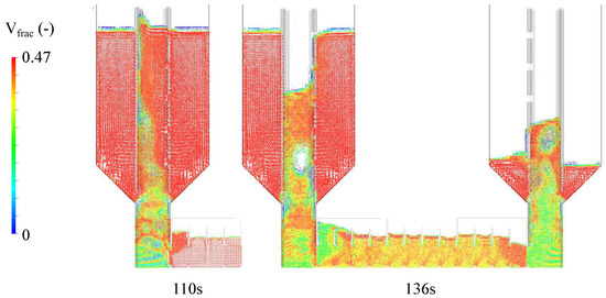
Figure 14.
Pipe 3—start-up and transport, —break-through in left hand side hopper at 110 s, sand is flowing through orifices at 136 s [20].
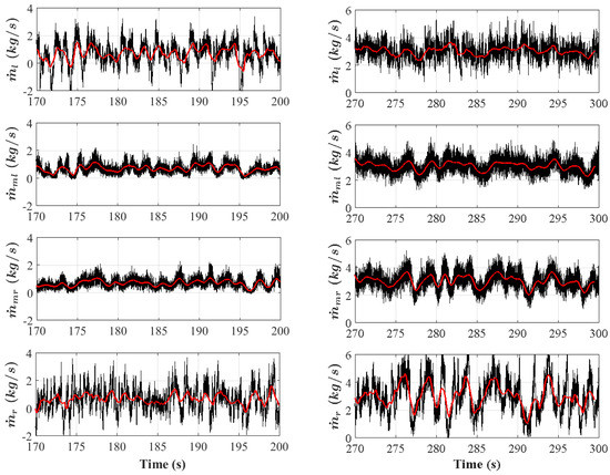
Figure 15.
Pipe 4—controlled particle mass flows (red: 1 s moving average), indexes refer to Figure 4 [22].
Pipe 4 seems to produce a higher pressure loss (respectively viscous friction), as the same gradients do yield lower mass flows compared to pipe 3. This higher pressure loss might well be the central stabilising factor regarding transport. The needed gradients for transport are still very small compared to the hydrostatic pressure increase along the risers. Thus, a controlled and mostly stable average mass flow of ≈0.7 kg/s is achieved. This refers to a mass flux of ≈21.7 kg/ms. Those range at the lower limits of feasible flows, respectively, fluxes with the chosen HEX cross section as significant horizontal (back-) mixing occurs at the HEX entry and exit (see blue regions in Figure 16). Still, plug flow with mostly negligible vertical and back mixing is demonstrated. The implementation of a tube bundle is expected to further improve this behaviour, while a longer HEX will render mixing phenomena in the in- and outlets irrelevant.
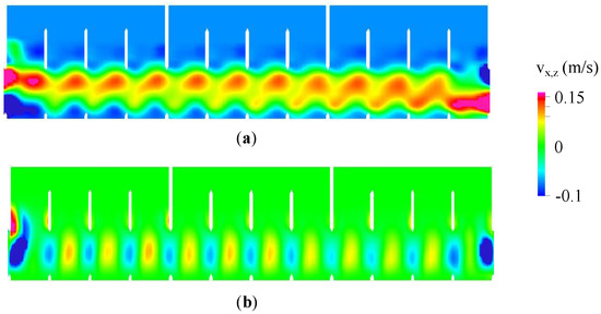
Figure 16.
Particle velocities averaged over approximately s in (a) horizontal () and (b) vertical () direction.
Another period of transport with : |1780 0 −1000| is performed and shown on the right hand side of Figure 15. It demonstrates that horizontal mixing fades with higher . This is attributed to the fact that horizontal particle mass flow oscillations introduced by the strongly bubbling beds of the risers remain approximately constant while the mass flow increases. In other words, the relative disturbance decreases and becomes insufficient to cause negative horizontal flow. With the described boundary conditions, a controlled and stable average mass flow of ≈3.1 kg/s is achieved. This refers to an impressive mass flux of ≈96.1 kg/ms. It is comprehensible to assume that yet higher mass fluxes could be realised. A tube bundle may limit those due to higher fluidic friction. Furthermore, a whole hopper volume is transported and the left hopper is totally emptied after a simulation time of roughly 400 s. Maximum s of |12 10 6 6 6 14 16| (see Figure 17) are applied. It seems the s have to be slowly and continuously increased with the level of the right hopper as its fluidisation tends to collapse with rising levels. This issue may possibly also be solved by pulsing fluidisation air. Fortunately seems to be not strongly influenced by this increase. Finally, it can be said that Pipe 4 or similar installations in the hoppers is a good solution for the challenges associated with control of stable mass flows and the transport into and out of powder storages located above the level of the HEX.
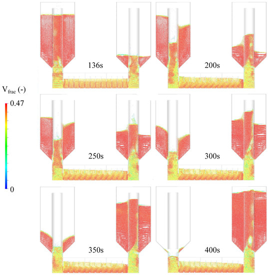
Figure 17.
Pipe 4—Transport of a whole hopper volume and total emptying of the left hopper at controlled goodmass flows of ≈3 kg/s, respectively, ≈0.7 kg/s [20].
Based on the simulations with pipe 4 a simple linear approach for the mass flow (Equations (3) and (5)) that roughly fits the results of and found in the numerical investigations may serve as an aid for calculation of assuming powder transport from left to right:
with being the essential degree of freedom for the user of the Matlab controller in Pa, Barracuda delivered Pa. may be seen as a static equilibrium criteria to balance the lift resulting from the fluidisation air introduced in the hoppers risers or, in other words, it is needed to prevent the HEX bulk from being sucked into the risers. Obviously this approach would need validation and calibration in experiments before it can be put to use. The impact of on is negligible as the HEX is very short in the presented numerical investigations to limit computational effort. This is expected to change significantly with a longer HEX in an industrial application.
5. Thermal Insulation
Bulk materials like quartz sand or corundum powder allow storage temperatures only limited by the strength of applied structural alloys at storage temperature. Thermal insulation is a critical parameter regarding the FP-TES layout. This is demonstrated with a short example: assuming, e.g., a hot storage hoppers surface temperature of = 850 C, an outside surface temperature of = 60 C and an ambient temperature of = 20 C, a cylindrical insulation layer thickness of mm is derived [34]. An insulation thickness of ≈563 mm would be applied at the bottom and cover of the hopper. Associated heat losses are 161 W/m. Between hoppers a thinner layer of high temperature insulation may be utilised in dependence of the cooler hoppers temperature.
Fortunately, this classic approach is too pessimistic in case of FP-TES, because the outer layers of the cylindrical bulk filling the hopper itself may be utilised as additional layers of insulation. The heat conductivity T) of the bulk itself is rather low, as it forms a porous medium consisting of greater than 50% air ((850 C) = 3.771 W/mK and (850 C) = 0.07477 W/mK). Thus, it is desirable to calculate and possibly arrive at a lower surface temperature without loosing much of the beds outer temperature. The prediction of thermal conductivities of packed beds has been a topic of intensive research for more than one century. Related methods that can be applied are found in [34]. Apparently primary parameters regarding have to be the beds porosity , the conductivity of the particles , and the conductivity of the fluid in between the particles . There are three basic types of approaches regarding this problem:
- Type I is to directly solve the Laplace equation for heat conduction for the beds conductivities and geometry, which is obviously extremely complex and will have to involve numerical methods mostly.
- Type II introduces thermal resistances in both phases and tries to combine them in a way that would represent wanted correlations (Ohmic analogs), for example, series or parallel arrangements of phases.
- Type III methods calculate the thermal conductivity of a unit cell, which is assumed representative for the whole bed. This can be seen as a compromise between the other two types and will yield sufficiently precise results at reasonable expense.
It seems a Type III method should be applied to approach the problem at hand—the model of Zehner, Bauer and Schlünder [34]. It introduces a unit cell consisting of a cylindrical core containing solid particles and a fluid-filled section around that core. The most basic version will be introduced in the following, as it is decided sufficiently precise for mostly spherical particles in a packed bed (e.g., quartz sand with a sphericity of 0.8). Nevertheless a more detailed examination of the topic including the more complex versions of this model and others is recommended for future work.
The basic model of Zehner, Bauer and Schlünder includes the following equations. The related heat conductivity is expressed as
with , where is the thermal conductivity of the unit cells core.
In Equation (8), is the particle heat conductivity and B a deformation parameter, and for spherical particles
If those equations are evaluated for both quartz sand and corundum powder, severe disadvantage regarding the utilisation of corundum powders with the FP-TES to this point is revealed. Obtained conductivities for are (850 C) = 0.352 W/mK and (650 C) = 0.285 W/mK, while the conductivities of are (850 C) = 0.663 W/mK and (650 C) = 0.513 W/mK, [20].
Apparently, the thermal conductivity of a packed bed composed of corundum powder is almost twice the value of a conductivity of a bed of quartz sand in the temperature range of interest, which is especially interesting as corundums’ thermal conductivities are more than thrice the values of quartz. This might substantially benefit quartz sand as a storage medium for longer storage durations, although further examinations regarding actual transient hopper temperature profiles (preferably in cylinder coordinates) and resulting conductivities and heat losses over time will be necessary. Nevertheless, the quartz sand beds thermal conductivities are roughly only twice as high as the conductivities of a common insulation material at the same temperatures, which means that the bed is half as good an insulation as the insulation itself, as conduction is linearly dependent on . Corundum powder could be an excellent storage medium for short term heat storage, where high energy densities are needed as its heat capacity is significantly higher compared to the quartz sand.
Further considerations and calculations regarding actual transient hopper temperature profiles (preferably in cylinder coordinates) and resulting heat losses over time should be performed. This should be achieved via a transient solution of the Laplace equation for a cylinder utilising -values obtained with the models of Zehner, Bauer and Schlünder [34].
6. Summary
To prove the concept of the FP-TES and to design the layout of a pilot plant, CPFD simulations are performed. In order to handle the control mechanism of the FP-TES—the varying pressure gradients—a transient simulation method is developed and tested on a preliminary layout. At first simplified geometries are investigated to prove the transport mechanism based on driving pressure gradients. However, those first geometries showed issues in terms of mixing and emptying the hoppers. Therefore, improved designs including rotational symmetric hoppers located above the HEX and additional baffles in the HEX are developed. To stabilise the fluidised bed in the hopper and ensure the desired emptying mechanism, various internal pipes are tested. It turns out that the application of a pipe with a vertical slot enables continues level equalisation between the pipe and the surrounding bed and is therefore the best choice.
A consideration of the thermal insulation revealed that the outer layer of the hopper should be taken into account. Using quartz sand as storage medium results in a thermal conductivity of the bed which is twice the value of common insulation material. Therefore, quartz sand would be an ideal choice for long term storage, while other materials with higher heat capacity and conductivity would be favourable for short time storage.
In Part II of this article, a validation of the numerical results by the use of a cold test rig is presented. Further calculations to fine tune the FP-TES design and evaluate the temperature profiles in the hopper should be performed in the future. Furthermore, one of the greatest challenges is to implement a reliable mass flow measurement to lay the foundation for the development of a control algorithm and prove the functionality of the FP-TES in a real industrial environment.
Author Contributions
Conceptualisation, D.W., V.S. and H.W.; methodology, D.W., V.S. and H.W.; software, D.W.; validation, V.S. and D.W.; writing—original draft preparation, D.W.; writing—review and editing, V.S. and H.W.; visualisation, D.W.; supervision, H.W.; project administration, H.W. and M.H.; funding acquisition, H.W., M.H. and V.S. All authors have read and agreed to the published version of the manuscript.
Funding
The authors would like to thank the FFG—Austrian Research Promotion Agency (FFG project number 858916) and the Austrian Wirtschaftsservice (prototype funding project number P1621702) for the financial support and funding of the conducted research work.The authors acknowledge TU Wien University Library for financial support through its Open Access Funding Programme.
Acknowledgments
Open Access Funding by TU Wien.
Conflicts of Interest
The authors declare no conflict of interest.
Abbreviations
The following abbreviations are used in this manuscript.
| Acronyms | |
| BC | Boundary Conditions |
| CPFD | Computational Particle Fluid Dynamics |
| FP-TES | Fluidisation-based Particulate—Thermal Energy Storage |
| FG | Fluidisation Grade |
| HEX | Heat Exchanger |
| IET | Institute for Energy-Systems and Thermodynamics |
| LES | Large Eddy Simulation |
| P2H2P | Power to Heat to Power |
| SGS | Smagorinsky Subgrid Scale |
| TES | Thermal Energy Storage |
| Latin Symbols | |
| A | Cross section, (m) |
| B | Deformation parameter, (-) |
| d | Diameter, (m) |
| g | Gravitational acceleration, () |
| h | Height, (m) |
| k | Ratio of thermal conductivity, (-) |
| Mass flow, () | |
| N | Model variable, (-) |
| p | Pressure, () |
| S | Sphericity, (-) |
| s | Thickness, (mm) |
| T | Temperature, (K) |
| t | Time, (s) |
| u | Velocity, (m/s) |
| V | Volume, (m) |
| Greek Symbols | |
| Pressure gradients, () | |
| Time difference, (s) | |
| Mass flux, () | |
| Thermal conductivity, () | |
| Density, () | |
| Porosity, (−) | |
| Indices | |
| a | Ambient |
| Cylindrical | |
| Driving | |
| Equilibrium | |
| f | Fluid |
| Fraction | |
| Heat exchanger | |
| hopper | |
| L | Left |
| M | Middle |
| Minimum fluidisation | |
| p | Particle |
| R | Right |
| W | Wall |
References
- Agency, I.E. Market Report Series: Renewables 2018; Technical Report; IEA: Paris, France, 2015. [Google Scholar]
- Balsalobre-Lorente, D.; Shahbaz, M.; Roubaud, D.; Farhani, S. How economic Growth, renewable Electricity and natural Resources contribute to CO2 Emissions. Energy Policy 2018, 113, 356–367. [Google Scholar] [CrossRef]
- Schwaiger, K.; Haider, M.; Steiner, P.; Hämmerle, M.; Wünsch, D. Fluidized Bed Facility and Method for Conveying a Solid Bulk Product. Austria WO Patent Application No. WO2020097657A1, 13 November 2019. [Google Scholar]
- Schwaiger, K. Development of a Novel Particle Reactor/Heat-Exchanger Technology for Thermal Energy Storages. Ph.D. Thesis, TU Wien, Vienna, Austria, 2016. [Google Scholar]
- Schwaiger, K.; Haider, M.; Haemmerle, M.; Wuensch, D.; Obermaier, M.; Beck, M.; Niederer, A.; Bachinger, S.; Radler, D.; Mahr, C.; et al. sandTES—An Active Thermal Energy Storage System Based on the Fluidisation of Powders. Energy Procedia 2014, 49, 983–992. [Google Scholar] [CrossRef]
- Steiner, P.; Schwaiger, K.; Walter, H.; Haider, M. Active fluidised bed technology used for thermal energy storage. In Proceedings of the ASME 2016 10th International Conference on Energy Sustainability collocated with the ASME 2016 Power Conference and the ASME 2016 14th International Conference on Fuel Cell Science, Engineering and Technology. American Society of Mechanical Engineers Digital Collection, Charlotte, NC, USA, 26–30 June 2016. [Google Scholar]
- Sakadjian, B.; Hu, S.; Maryamchik, M.; Flynn, T.; Santelmann, K.; Ma, Z. Fluidized-bed technology enabling the integration of high temperature solar receiver CSP systems with steam and advanced power cycles. Energy Procedia 2015, 69, 1404–1411. [Google Scholar] [CrossRef][Green Version]
- Rovense, F.; Reyes-Belmonte, M.; González-Aguilar, J.; Amelio, M.; Bova, S.; Romero, M. Flexible electricity dispatch for CSP plant using un-fired closed air Brayton cycle with particles based thermal energy storage system. Energy 2019, 173, 971–984. [Google Scholar] [CrossRef]
- Farsi, A.; Dincer, I. Thermodynamic assessment of a hybrid particle-based concentrated solar power plant using fluidised bed heat exchanger. Solar Energy 2019, 179, 236–248. [Google Scholar] [CrossRef]
- Ma, Z.; Davenport, P.; Zhang, R. Design analysis of a particle-based thermal energy storage system for concentrating solar power or grid energy storage. J. Energy Storage 2020, 29, 101382. [Google Scholar] [CrossRef]
- Gomez-Garcia, F.; Gauthier, D.; Flamant, G. Design and performance of a multistage fluidised bed heat exchanger for particle-receiver solar power plants with storage. Appl. Energy 2017, 190, 510–523. [Google Scholar] [CrossRef]
- Karimipour, S.; Pugsley, T. Application of the particle in cell approach for the simulation of bubbling fluidised beds of Geldart A particles. Powder Technol. 2012, 220, 63–69. [Google Scholar] [CrossRef]
- Liang, Y.; Zhang, Y.; Li, T.; Lu, C. A critical validation study on CPFD model in simulating gas–solid bubbling fluidised beds. Powder Technol. 2014, 263, 121–134. [Google Scholar] [CrossRef]
- Chen, C.; Werther, J.; Heinrich, S.; Qi, H.Y.; Hartge, E.U. CPFD simulation of circulating fluidised bed risers. Powder Technol. 2013, 235, 238–247. [Google Scholar] [CrossRef]
- Kraft, S.; Kirnbauer, F.; Hofbauer, H. CPFD simulations of an industrial-sized dual fluidised bed steam gasification system of biomass with 8 MW fuel input. Appl. Energy 2017, 190, 408–420. [Google Scholar] [CrossRef]
- Bandara, J.C.; Thapa, R.; Nielsen, H.K.; Moldestad, B.M.E.; Eikeland, M.S. Circulating fluidised bed reactors–part 01: Analyzing the effect of particle modelling parameters in computational particle fluid dynamic (CPFD) simulation with experimental validation. Part. Sci. Technol. 2020, 1–14. [Google Scholar] [CrossRef]
- Watanabe, N.; Kubo, M.; Yomoda, N. An 1D-3D Integrating Numerical Simulation for Engine Cooling Problem; Technical Report; SAE Technical Paper: Detroit, MI, USA, 2006. [Google Scholar]
- Arendt, K.; Krzaczek, M. Co-simulation strategy of transient CFD and heat transfer in building thermal envelope based on calibrated heat transfer coefficients. Int. J. Therm. Sci. 2014, 85, 1–11. [Google Scholar] [CrossRef]
- Unterluggauer, J.; Doujak, E.; Bauer, C. Numerical fatigue analysis of a prototype Francis turbine runner in low-load operation. Int. J. Turbomach. Propuls. Power 2019, 4, 21. [Google Scholar] [CrossRef]
- Wünsch, D. Advanced Regenerator: A Counter-Current Fluidized Bed Regenerator Utilizing a Pressure Gradient for Powder Transport. Master’s Thesis, TU Wien, Vienna, Austria, 2016. [Google Scholar]
- Sulzgruber, V.; Wünsch, D.; Haider, M.; Walter, H. FP-TES: A Fluidisation Based Particle Thermal Energy Stotage, Part II: Numerical Investigations. Energies 2020. Submitted. [Google Scholar] [CrossRef]
- Sulzgruber, V.; Wünsch, D.; Haider, M.; Walter, H. Numerical investigation on the flow behaviour of a novel fluidisation based particle thermal energy storage (FP-TES). Energy 2020, 200, 117528. [Google Scholar] [CrossRef]
- Yang, W.C. Handbook of Fluidization and Fluid-Particle Systems; CRC Press: Cleveland, OH, USA, 2003. [Google Scholar]
- Rhodes, M.J. Introduction to Particle Technology; John Wiley & Sons: Hoboken, NJ, USA, 2008. [Google Scholar]
- Frazzica, A.; Cabeza, L.F. Recent Advancements in Materials and Systems for Thermal Energy Storage: An Introduction to Experimental Characterization Methods; Springer: Heidelberg, Germany, 2018. [Google Scholar]
- Calderón, A.; Barreneche, C.; Palacios, A.; Segarra, M.; Prieto, C.; Rodriguez-Sanchez, A.; Fernández, A.I. Review of solid particle materials for heat transfer fluid and thermal energy storage in solar thermal power plants. Energy Storage 2019, 1, e63. [Google Scholar] [CrossRef]
- O’Rourke, P.J.; Snider, D. An improved Collision Damping Time for MP-PIC Calculations of dense Particle Flow with Applications to polydisperse sedimenting Bed Sand colliding Particle Pets. Chem. Eng. Sci. 2010, 65, 6014–6028. [Google Scholar] [CrossRef]
- Snider, D. Three fundamental granular Flow Experiments and CPFD Predictions. Powder Technol. 2007, 176, 36–46. [Google Scholar] [CrossRef]
- Wen, C.; Yu, Y. Mechanics of Fluidisation. Chem. Eng. Prog. Symp. 1966, 62, 100–111. [Google Scholar]
- Yang, W.C.; Dekker, A.O. (Eds.) Handbook of Fluidisation and Fluid-Particle Systems; CRC Press: New York, NY, USA, 2003. [Google Scholar]
- Smagorinsky, J. General Circulation Experiments with the Primitive Equations. I. The Basic Experiment. Mon. Weather. Rev. 1963, 91, 99–164. [Google Scholar] [CrossRef]
- Hain, K. The partial Donor Cell Method. J. Comput. Phys. 1987, 73, 131–147. [Google Scholar] [CrossRef]
- Schulze, D. Powders and Bulk Solids: Behavior, Characterization, Storage and Flow Schulze, Dietmar; Springer: Berlin/Heidelberg, Germany, 2014. [Google Scholar]
- Kind, M.; Martin, H.; Stephan, P.; Roetzel, W.; Spang, B.; Müller-Steinhagen, H.; Luo, X.; Kleiber, M.; Joh, R.; Wagner, W.; et al. VDI Heat Atlas; VDI Gesellschaft Verfahrenstechnik und, Ed.; Springer: Heidelberg, Germany, 2010. [Google Scholar]


© 2020 by the authors. Licensee MDPI, Basel, Switzerland. This article is an open access article distributed under the terms and conditions of the Creative Commons Attribution (CC BY) license (http://creativecommons.org/licenses/by/4.0/).