Article

Willow Biomass Crops Are a Carbon Negative or Low-Carbon Feedstock Depending on Prior Land Use and Transportation Distances to End Users

1
Department of Environmental Resources Engineering, State University of New York College of Environmental Science and Forestry, Syracuse, NY 13210, USA
2
Department of Sustainable Resources Management, State University of New York College of Environmental Science and Forestry, Syracuse, NY 13210, USA
3
Department of Civil and Environmental Engineering, University of California, Merced, CA 95343, USA
*
Author to whom correspondence should be addressed.
Energies 2020, 13(16), 4251; https://doi.org/10.3390/en13164251
Submission received: 4 July 2020 / Revised: 7 August 2020 / Accepted: 11 August 2020 / Published: 17 August 2020

Abstract

:
Few life cycle assessments (LCAs) on willow biomass production have investigated the effects of key geographically specific parameters. This study uses a spatial LCA model for willow biomass production to determine spatially explicit greenhouse gas (GHG) emissions and energy return on investment (EROI), including land use conversion from pasture and cropland or grassland. There were negative GHG emissions on 92% of the land identified as suitable for willow biomass production, indicating this system’s potential for climate change mitigation. For willow planted on cropland or pasture, life cycle GHG emissions ranged from −53.2 to −176.9 kg CO2eq Mg-1. When willow was grown on grassland the projected decrease in soil organic carbon resulted in a slightly positive GHG balance. Changes in soil organic carbon (SOC) associated with land use change, transportation distance, and willow yield had the greatest impacts on GHG emissions. Results from the uncertainty analysis exhibited large variations in GHG emissions between counties arising from differences in these parameters. The average EROI across the entire region was 19.2. Willow biomass can be a carbon negative or low-carbon energy source with a high EROI in regions with similar infrastructure, transportation distances, and growing conditions such as soil characteristics, land cover types, and climate.

Graphical Abstract

1. Introduction

Over several decades in North America and Europe, short rotation woody crops (SRWC), such as willow and poplar, have been increasingly recognized as important renewable energy sources because of their multiple environmental and rural development benefits. As a low-carbon energy source, willow biomass is helpful in decreasing greenhouse gas (GHG) emissions when it is used to replace fossil fuels, benefitting local rural communities by providing employment and improving energy independence, and providing multiple ecosystem services by decreasing soil erosion, improving water quality, and increasing biodiversity [1,2,3]. For example, willow can support biodiversity by functioning as natural habitats or as ecological corridors connecting patches in increasingly fragmented landscapes in the US [4]. In some situations, there are concerns that large scale deployment of willow could impact landscape aesthetics and diversity if a large proportion of one particular land type, such as natural grassland, in a given areas is converted to willow. The most recent US Billion-Ton report projected that 411 million to 736 million dry tons of energy crops, including willow, could be produced annually in 2040 with a price of $60 per dry Mg or less under baseline and high-yield case assumptions, respectively [5]. New York State recently adopted aggressive goals to reduce greenhouse gas emissions by 85% by 2050 [6,7].
Environmental indicators of renewable energy systems include GHG emissions, productivity of bioenergy crops [8], and energy return on fossil fuel inputs. Life cycle assessment (LCA) is a widely accepted method used to quantify the environmental impacts for processes or products across their life cycle. LCA is a tool used to assess the GHG emissions and other environmental impacts of bioenergy crop production including cultivation, harvesting, and transporting biomass to end users [9,10,11]. In addition, in the US Energy Investment and Security Act (P.L. 110–140, subtitle A), LCA has been identified as the standard methodology to determine if biofuels meet requirements for GHG reductions required for the National Renewable Fuel Standard.
In North America and Europe, a large number of studies have used LCA to evaluate environmental impacts and energy return on energy investment (EROI) of willow biomass crop production. Djomo et al. (2011) reviewed 26 papers and reported that the range of EROI for willow was between 3:1 and 16:1 and GHG emissions ranged from 0.7 to 10.6 g CO2 MJ−1 at the farm gate [9]. Since 2011, additional LCAs on willow crop production systems have been conducted for the US [1], Asia [12], and Europe [13,14,15]. The EROI in these studies ranges from 11.0:1 to 43.4:1 for willow biomass delivered to facility that converts the biomass to bioenergy, biofuels, or bioproducts.
The life cycle GHG emissions range from 33.7 to 100 kg CO2eq per oven dry Mg of willow chip production including delivery to power plants without including belowground carbon sequestration, or changes in soil organic carbon (SOC) associated with land use change (LUC) [10,16,17]. However, it has been demonstrated that belowground carbon, (i.e., carbon sequestered in the coarse roots and stool) is substantial [18] and can reduce GHG emissions by as much as 138.4 kg CO2eq per Mg biomass [1]. Results of SOC changes under willow cultivation are inconclusive to date in New York State because changes have only been measured at a limited number of sites [19]. Recently, detailed studies have been conducted by Argonne National Laboratory to predict SOC change associated with LUC using the CENTURY model, thus providing estimates of this critical component of GHG emissions of bioenergy crop feedstock production [20,21]. However, LCAs that incorporate SOC changes in willow feedstock production have been lacking in the US.
In previous LCAs that did not include changes in SOC, the three largest contributors to the life cycle GHG emissions are fertilization, transport, and harvesting [11,14,16,17,22,23,24]. In two LCAs that include SOC change in Sweden, yield was found to be the most important factor for climate change mitigation [13,14]. These four factors are subject to a large magnitude of uncertainty in LCA of willow production in different geographical locations [1,14,20,21]; therefore, incorporating spatial variability in LCA modeling is one approach to address this uncertainty. An LCA that considered spatial variability and changes in SOC content had an average EROI of 30:1 and determined that 84.3 Mg carbon ha−1 would be sequestered in the soil during a 100-year time frame in Sweden [14]. However, studies with SOC change from land use changes with finer spatial scales that can incorporate more variability on landscape levels are lacking in the US and other parts of the world.
The objectives of this study were to conduct spatial LCA of willow biomass production and delivery of chips to an end user including SOC change and location-specific modeling of GHG emissions and fossil fuel consumption to investigate variations across five counties in central and northern New York State. In this study, biomass growth data from 480 ha willow biomass crops and other recently collected primary and GIS data from the region were used as data sources to create an LCA model of willow biomass production that yields cradle-to-gate GHG emissions and EROI.

2. Materials and Methods

2.1. Scope of LCA and Life Cycle Inventory

A baseline LCA model for willow supply chain system was generated in SimaPro 8.2 using inventories from the Ecoinvent 3.3 and USLCI databases. The goal of the LCA was to estimate GHG emissions and the energy balance of willow production in New York State including direct land use change, with willow cultivation starting on land currently classified as either pasture or cropland as separate scenarios. The scope of the LCA includes the nursery and the main production system as two stages of the supply chain and ends with the delivery of willow chips to the plant gate of an end user (Figure 1). Within the boundaries for this study only direct land use change (i.e., when land used for a specific purpose like crop production is converted to another use, willow production in this paper) is considered. This study assesses the global warming impact and energy balance, because these two attributes are critical to evaluate willow biomass as a source of renewable energy. The geographic boundaries of this analysis include suitable lands for growing willow in five counties in central and northern New York State (NY), namely Oneida, Jefferson, Oswego, Lewis, and St. Lawrence (Figure 2), where two facilities have used willow for a portion of their fuel supply for power and heat production. The temporal boundaries cover seven 3-year rotations of growing and harvesting willow crop within 22 years, including one site preparation year. Data supports consistent willow production over seven rotations [18] and this timespan has been used for previous LCAs [1] in the region. The LCA includes all equipment usage and materials consumption, e.g., tractor use and diesel.
The functional unit of this LCA is one oven-dry Mg of willow biomass chips delivered to an end user. This function unit was chosen because mass is commonly used in the field and is used in willow LCA [1,4,9] which is an important factor in this study. This functional unit choice matches the cradle-to-gate scope of this LCA and allows for the results to be subsequently used in future LCAs that extend the scope to bioenergy production.
All life cycle inventories used in the LCA model are from the Ecoinvent database and USLCI database (Table S1), including mowing, fertilizing, planting, harvesting, and transporting chips, with necessary adjustments according to field operations. For example, the harvesting process in willow production is modeled by computing hourly diesel consumption (95.4 L h−1 [25]) and including forestry harvester production adjusted for a total of 5000 working hours of the forage harvester from interviewing an equipment expert. The planting process in Ecoinvent 3 has the planting rate of 5 tractor hours ha−1 compared to 1 h ha-1 that has been measured for planting willow in this region [26]. Therefore, a ratio of 0.2 was applied to the planting process in Ecoinvent 3 to represent the process of planting willow cuttings. The baseline estimates of environmental impacts in kg CO2eq of these processes were calculated by the EPA TRACI 2.1 life cycle impact assessment method using SimaPro 8.2 based on the mean values of modeled input parameters. The baseline energy balance in MJ (nonrenewable fossil fuels) for each process was computed by the cumulative energy demand life cycle impact assessment method. The energy content of willow biomass, GHG emissions per unit energy consumption, e.g., CO2 per MJ, and EROI were based on the higher heating value (HHV) of 19.6 GJ Mg−1 of willow biomass [27].
The key parameters determining the energy and material consumption of the system are listed in Table 1. The baseline values are used for calculations for each field. The sensitivity analysis of the model was conducted using Python code for key parameters that have at least 10% contribution to the total impact or have impacts on multiple processes listed in Table 1 (e.g., yield, which affects both transport and belowground biomass). The process of sensitivity analysis starts with varying one parameter at a time while keeping all the other parameters constant, and the resulting ranges of environmental impact values represent the level of sensitivity of the LCA results to the specific parameter. Sensitivity analyses were conducted separately for pasture and cropland scenarios in the five counties. The minimum and maximum parameter values are 80% and 120% of baseline values to place a benchmark for comparisons among parameters, except for the wagon number, with a minimum of one and a maximum of three, and transportation distances.
Uncertainty analysis aims to include all factors’ probability distribution functions (PDFs) at once to determine the PDF of LCA results. Uncertainty analysis was also conducted in Python code to evaluate the probability of environmental impacts when the uncertainties of all key parameters are included in the model. The code randomly drew parameter values from uniform distributions and ran the model 10,000 times to obtain resulting PDFs for each scenario. Each parameter was assumed to be uniformly distributed and the ranges of variation for each parameter were determined based on expert knowledge, GIS analysis, and the existing scientific literature (Table 1).

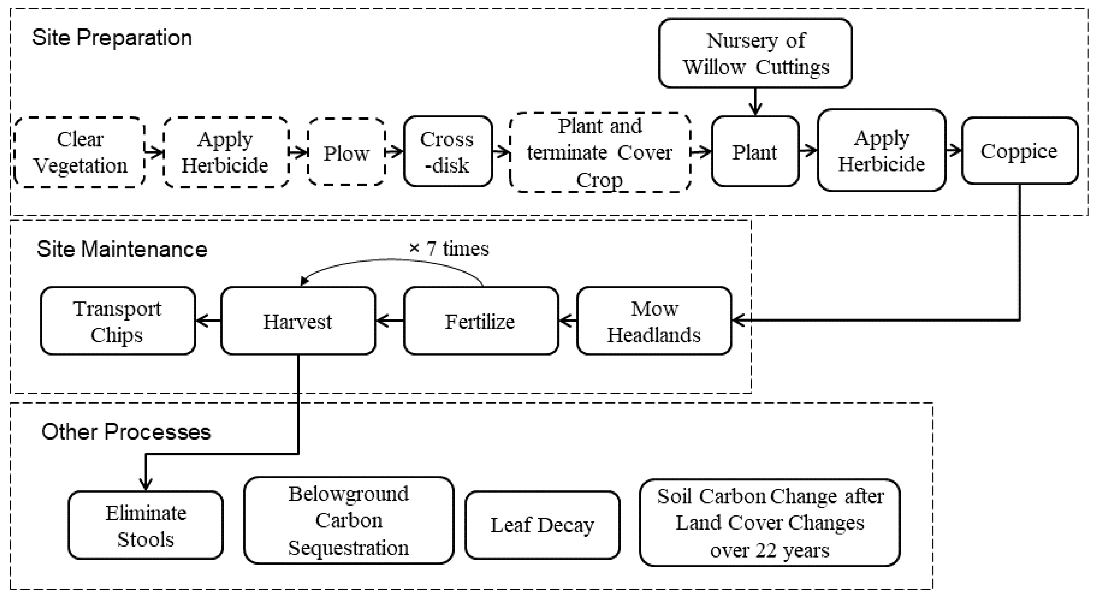
2.2. Willow Supply Chain System

To accurately depict the system for this LCA, a comprehensive list of field operation steps and processes in the willow production supply chain system as well as details of each process, e.g., application rates, machineries, material, and fuel consumption, were obtained from previous literature or through interviewing experts of willow biomass production who are working on the 480 ha willow biomass crops in central and northern NY (Figure 1, Table S1). The willow production system starts with a nursery system of willow cuttings as described in a previous study [1]. For existing grassland, the main production system starts with site preparation in the first and second year of establishment, including clearing existing vegetation, herbicide, plowing, disking, rock-picking, sowing and terminating cover crop, and planting willow cuttings. For a conservative estimate, all grassland parcels were assumed to have lower soil pH values and rocks so lime additions and picking rock were applied in these parcels. For cropland, most site preparation steps are not necessary except cross-disking. The willow shoots are coppiced after the first growing season. At the end of every 3-year rotation, willow stems are harvested with a single pass cut and chip system, blown into wagons, loaded to trucks, and transported to end users. There are seven consecutive 3-year rotations modeled, and following the final harvest, the re-sprouting crop is sprayed with herbicide and the stools are ground down. Fertilizer is applied at 100 kg N ha−1 in urea once every 3 years at the beginning of each rotation. Headlands around the field are mowed annually but there are no other regular field activities (Figure 1).
The nitrous oxide emissions from leaf decay are calculated based on the method by the Intergovernmental Panel on Climate Change (IPCC) 2006 which takes into account the total amount of leaf litter and the nitrogen content in leaf biomass assuming that 1% of leaf biomass leads to nitrous oxide emissions over 22 years [30]. In addition, nitrous oxide emissions were computed as 1% of applied fertilizer, i.e., 1 kg nitrous oxide per 100 kg N applied in the field and of N contributed in leaf fall. The amount of N contributed from foliage was calculated from leaf biomass based on the leaf/shoot biomass ratio, aboveground biomass yield, and N concentration reported by Sleight et al. (2015) [31]. In addition, the amount of belowground carbon sequestration is obtained by applying the root/shoot ratio by Sleight et al. (2015) and using the aboveground biomass yield [31]. For example, out of an entire willow plant, shoots comprise 50.8% of biomass, whereas aboveground stool, belowground stool, and coarse root are 30.7% biomass. This results in a root/shoot ratio of 0.6 and belowground biomass of 18 Mg/ha including coarse roots and stools given an aboveground yield of 30 Mg ha−1 in a rotation. Carbon sequestration in fine roots cycles several times per year so it is not included in the belowground carbon pool [18]. The root/shoot ratio in Sleight et al. (2015) is based on the data from the third year of the third rotation [31]. The amount of root biomass usually levels off or may slightly increase after the third rotation or 12–14 years [32], so belowground biomass is no longer accumulated after the third rotation, which leads to a conservative estimate of belowground carbon in this study. Finally, after seven 3-year rotations, the willow crop is ended by harvesting, applying herbicide, and grinding the stools into the soil; therefore, roots and belowground stools are counted as additions to belowground carbon sequestration within the time scope of this study.
In addition, the analysis includes the processes of SOC changes associated with direct land use change (LUC). Indirect LUC is not considered in this study because relevant factors, such as policy, markets, food production technology improvement, and other factors that impact indirect LUC, are outside the scope of this study. The amount of SOC change was determined for four scenarios separately including two starting land cover categories, namely grassland and cropland, and two soil depths, 30 and 100 cm, corresponding to the SOC data available from Qin et al. (2016a) and Qin et al. (2016b) [20,21]. This SOC data from Argonne National Lab is based on 30-year annualized change from 2011 to 2040 in Mg C ha−1 yr−1, and we applied this SOC rate over 22 years, which is the temporal scope of this study. In addition, there are multiple scenarios in the SOC data. For example, Qin et al. assume that the land was either in grassland or pasture for 130 years prior to being converted to willow, and in yield-increase or yield-constant scenarios [20,21]. In this study, we averaged data over all scenarios in the two LUC scenarios of cropland and grassland to willow. Although there are spatial resolution differences between SOC data and land use data, the current resolution of SOC data, which is at the county scale, is sufficient for between county variation analysis. We included an indication of the spatial resolution of the different datasets (Table 2). In all cases, we selected the finest scale resolution available to capture the variation of the changes in GHG and EROI across the landscape. The soil change data from Qin et al. (2016 a & b) and Dunn et al. (2014) is available at the county level for two different land use change scenarios—from annual crops to willow or from grassland/pasture to willow—and for two different soil depths—to 30 cm and to 100 cm depths [20,21,33]. We applied these results using the land uses that were identified using the 2011 National Land Cover Database (NLCD) data, which is available at a resolution of 30 m, to allow us to look at potential land use change impacts at a resolution finer than the county.

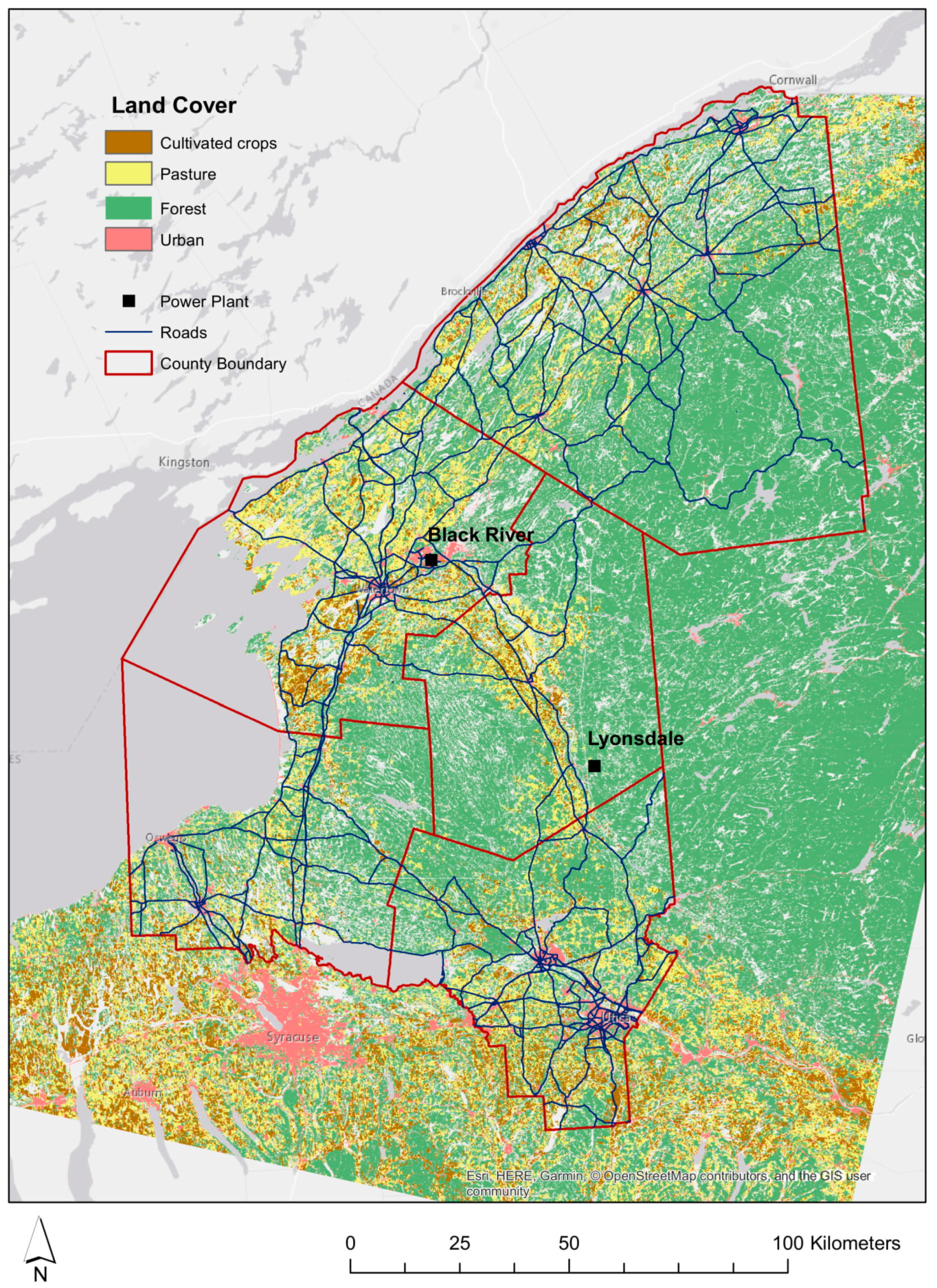
2.3. Identification of Suitable Lands for Willow Crops in GIS

The GIS analysis for the identification of suitable lands for potential willow crops is based on multiple datasets to select and process parcels through a range of criteria. First, land cover information was obtained from the 2011 NLCD [34], which has an overall accuracy of 88% on level I Anderson classification [35]. Second, the slopes of parcels were derived from elevation data with 1 arc-second or approximately 30 m resolution developed by the U.S. Geological Survey (USGS) National Geospatial Program (https://www2.usgs.gov/ngpo/). Third, hydrology data were derived from Cyber Security and Critical Infrastructure Coordination (CSCIC) Accident Location Information System (ALIS) database (https://gis.ny.gov/gisdata/) including both linear and areal maps representing rivers and lakes, respectively. Fourth, the soil data were derived from the SSURGO soil database including soil attributes such as soil types and productivity in a 10 m resolution raster map covering New York State. Fifth, tax parcel data were obtained from property tax offices in each county in vector format with land use code and polygon representing land use types and boundaries for each tax parcel. Finally, the road network data in New York State were derived from the Topologically Integrated Geographic Encoding and Referencing (TIGER) dataset containing primary and secondary roads available from the US Census Bureau. Spatial resolutions of raster data are summarized in Table 2. SSURGO soil data of 10 m resolution was generalized to 30 m to conform to the spatial resolution of land cover, elevation, and slope data. All resulting data layers were averaged and applied within parcel boundaries. In addition, soil carbon data were applied to parcels based on which county a parcel is located. These data were processed using the Spatial Analyst toolbox in ArcGIS 10.1 developed by Environmental Systems Research Institute, Inc. (Redlands, CA, USA). The suitable lands for willow crop in this study are generated based on multiple criteria regarding land cover, land use classes, slope, water areas, and spatial connectivity (Figure S1). This method improved the GIS model for generating suitable lands in Castellano et al. (2009) by excluding scattered lands less than 8 ha after examining spatial continuity [36]. The suitable lands also excluded slopes greater than 8% due to limitations for forage harvesters that are used to harvest willow and water/wetland areas. The resulting suitable lands include four land cover classes of shrub/scrub, grassland, pasture, and cropland in tax parcels of agricultural land use corresponding to land cover class codes of 52, 71, 81, and 82, respectively, in Anderson land cover classification system in the NLCD dataset. The land cover class for a given parcel is determined by majority rule; the parcel is assigned to the land cover class with highest proportional coverage in the parcel. The transportation distance from suitable lands to one of two end users in the region was calculated based on road network data of primary and secondary roads where trucks are allowed using Network Analyst in ArcGIS. The biomass yields of willow in suitable lands in each parcel were estimated by the equation in the Renewable Fuels Roadmap Appendix E and scaled to dry Mg ha−1 based on the National Commodity Crop Productivity Index (NCCPI) contained in SSURGO soil layers [37]. The equation is based on yield data from the field and can be validated. NCCPI applies natural relationships of soil, landscape, and climate factors to model the productivity of commodity crops. The equation (1) for estimating willow yield is
Yield (ODT ac−1 yr−1) = (50.5 + 119 × NCCPI + 1.275 × 5) × 0.028 × 2 × 0.845 × 0.9273,
where mean NCCPI values of each parcel were input from soil data layer and utilized in the equation to provide the amount of oven dry ton (ODT) willow biomass per year per acre. NCCPI was used to estimate willow yields because the SSURGO data is available at a finer resolution than other yield recent yield estimates at a coarser scale [38].
The maps of land cover changes were generated by comparing original land cover maps with the suitable lands to examine types of land covers in each suitable parcel to be converted to willow. The land cover information is necessary to determine SOC change after willow establishment due to different rate of SOC change in conversion of grassland and cropland [20,21] and used to allocate site preparation activities. The resulting maps of land cover change, biomass yield, and transportation distance for suitable parcels set the stages for the LCA scenarios.

2.4. LCA Modeling on Landscape Scales

The LCA model in this study incorporates spatial variations of input parameters based on the GIS analysis results. The LCA model includes parameters with high spatial variability including (1) willow yield, (2) transportation distance from farm gate to power plants, (3) the land use conversion process when establishing willow crops related to different site preparation processes, and (4) SOC change in grassland and cropland. For SOC change modeling, the grassland case includes land designated as shrub and grassland in NLCD data, and the cropland case includes pasture and cropland in NLCD data. The annual SOC change rate is shown in Table 3, in which SOC changes were modeled separately for the five counties over 22 years. We applied Argonne’s work as our input data shown in Table 3 and averaged it by the willow production over 21 years in the two LUC scenarios (grassland to willow and cropland to willow) in two soil depths of 30 and 100 cm. For example, in the original Argonne data sets, Jefferson county in New York State has −0.19 and −0.31 Mg C ha−1 yr−1 for yield increase and yield constant scenarios, respectively, for pasture to willow LUC. The average of the two is a loss of soil carbon at the rate of −0.25 Mg C ha−1 yr−1, which is the rate used in our model. The one-way transportation distance from each parcel to the closest end user was doubled in the LCA model to account for a roundtrip to and from the end user. These parameters vary across tax parcels and by land cover types; therefore, separate baseline LCA scenarios were analyzed for each parcel across the five counties to determine variations of environmental impacts within the counties. In addition, spatial variations were also incorporated in the sensitivity analysis of the LCA model. Sensitivity analysis and uncertainty analysis were conducted separately for each of the five counties.

3. Results

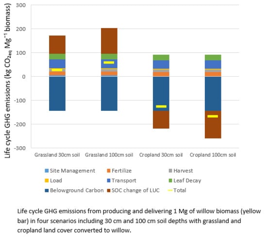
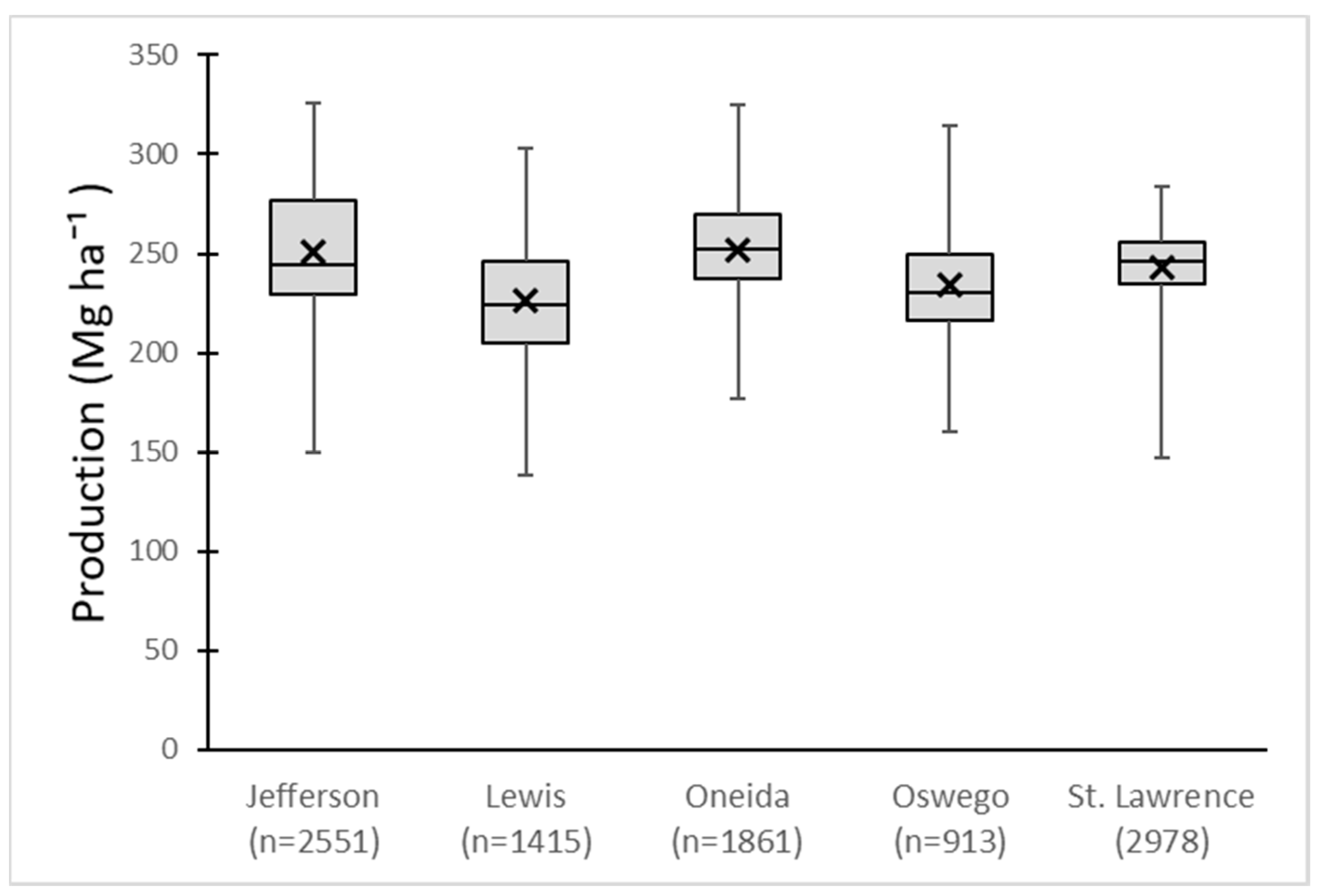
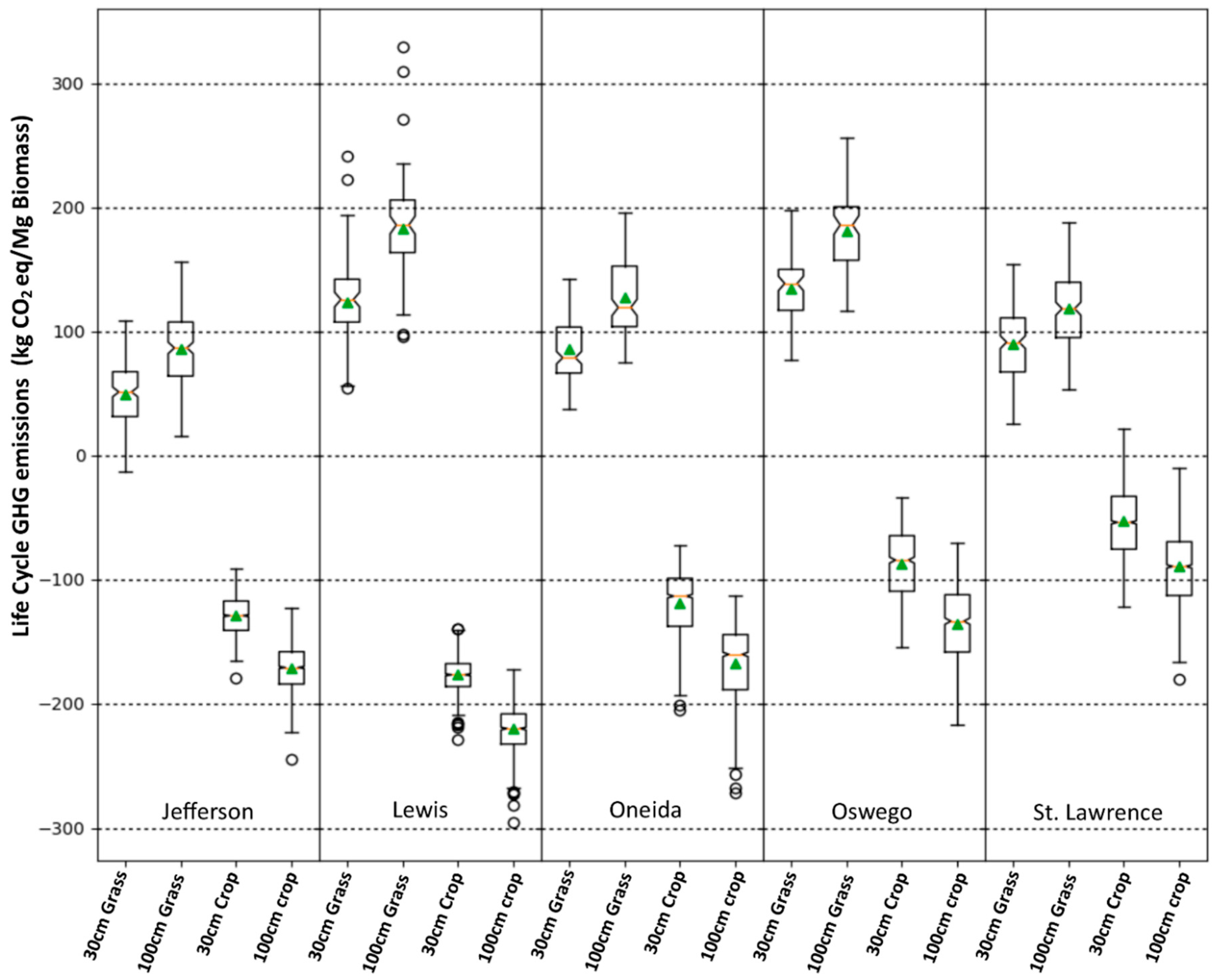
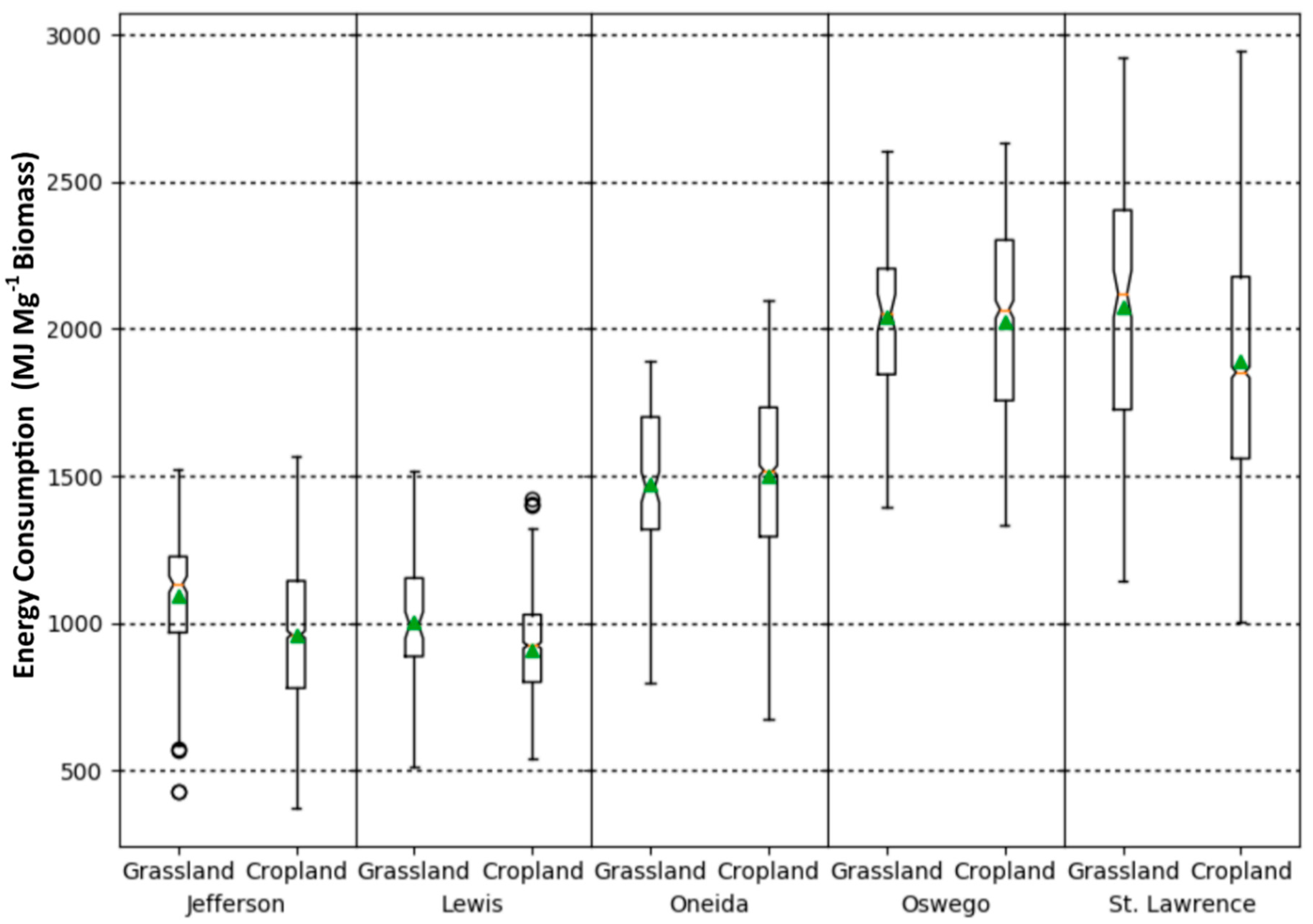
3.1. Baseline LCA Results

The baseline LCA results show differences in the life cycle GHG emissions in multiple scenarios of land cover and soil depths. Using the baseline parameters in Table 1, the life cycle GHG emissions of producing and delivering 1 Mg biomass are 27.7 kg CO2eq on grassland converted to willow including SOC change within 30cm soil depth over 22 years (Figure 3). The number decreases to −126.8 kg CO2eq Mg−1 biomass (a net sequestration of carbon for the cradle-to-gate system) when willow is grown on cropland or pasture due to the different SOC change rate in 30-cm soil. The difference between cropland and pasture, due to less site preparation in cropland, is 2.43 kg CO2eq Mg−1, which is minor compared with the SOC change difference. For a 100-cm soil depth, the total life cycle GHG emissions are 58.7 kg CO2eq Mg−1 for grassland and −167.1 kg CO2eq Mg−1 for cropland. The increased magnitudes are the results of higher rates of SOC change in deeper soil. Based on the energy content of 19.6 GJ Mg−1 for willow biomass [27], the emission factor, or amount of GHG emissions per GJ, is 1.4 kg CO2 GJ−1 for the 100-cm grassland scenario and it is −6.5 kg CO2 GJ−1 for the 100 cropland scenario. The energy consumption for the production process in grassland is 969.6 MJ for 1 Mg biomass (Figure S2) and the net EROI is 19.2. For cropland, this number decreased to 937.9 MJ for 1 Mg biomass and the EROI increased to 19.8 due to fewer steps in the site preparation process.
Transportation is the largest energy investment in the system, accounting for 540.3 MJ for 1 Mg biomass which is 55.7% of total energy consumption of the grassland scenario (Figure S2), for the 62-km roundtrip to and from the end user which is the average distance in Jefferson County (Table 1). Harvesting and fertilizing are the next two largest energy inputs, accounting for 139.8 and 164.6 MJ Mg−1, or 14% and 17% of the total energy consumption of grassland scenario, respectively.

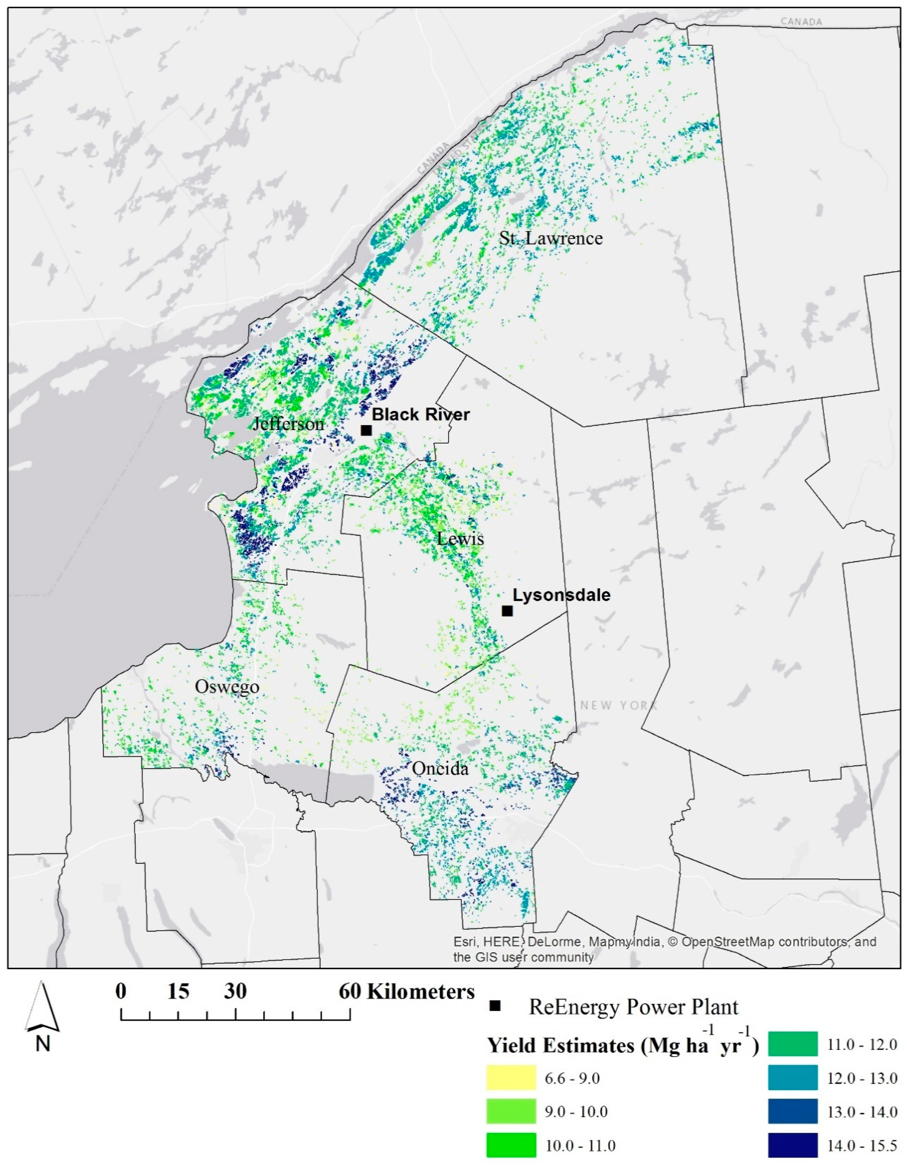
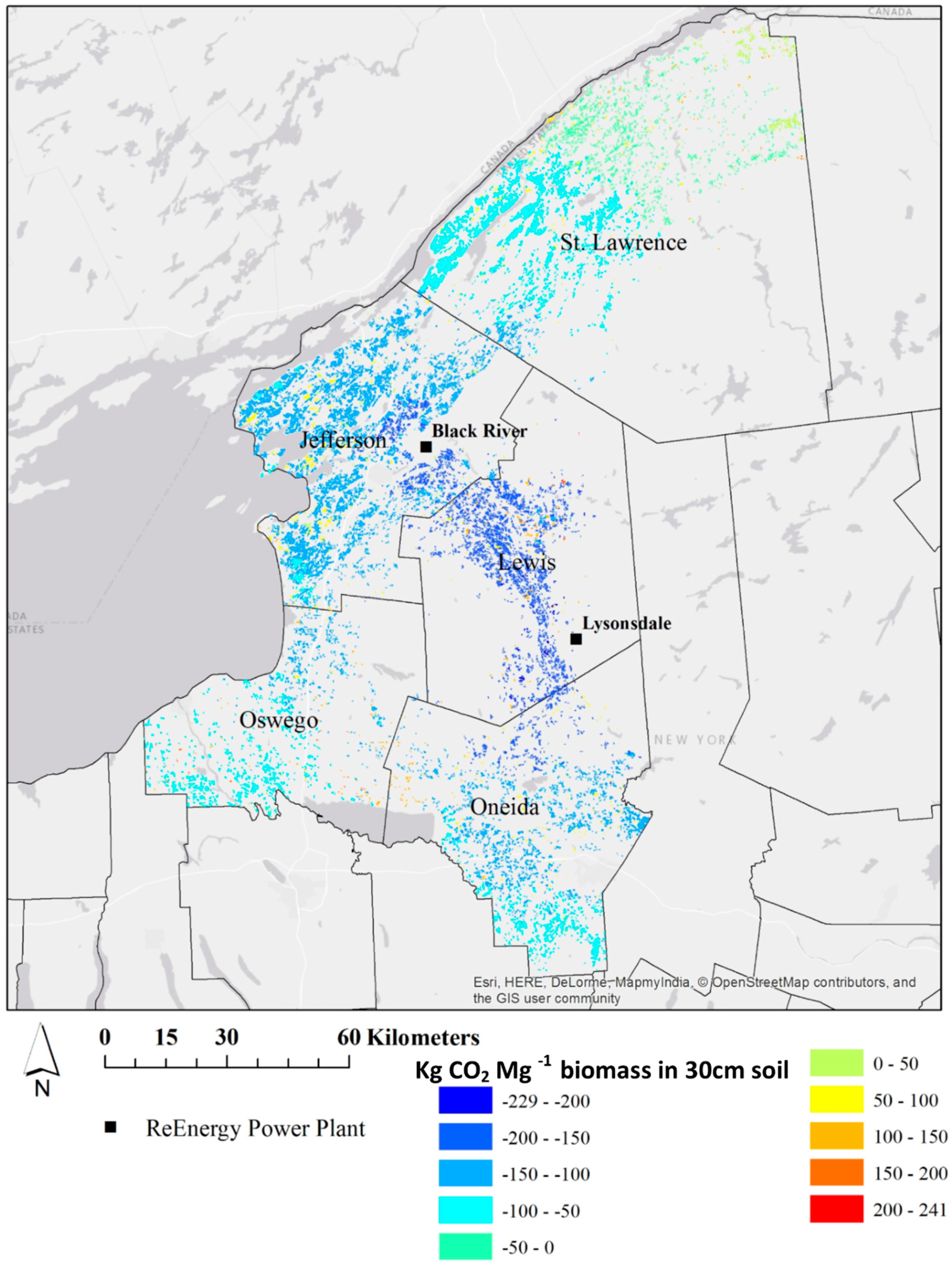
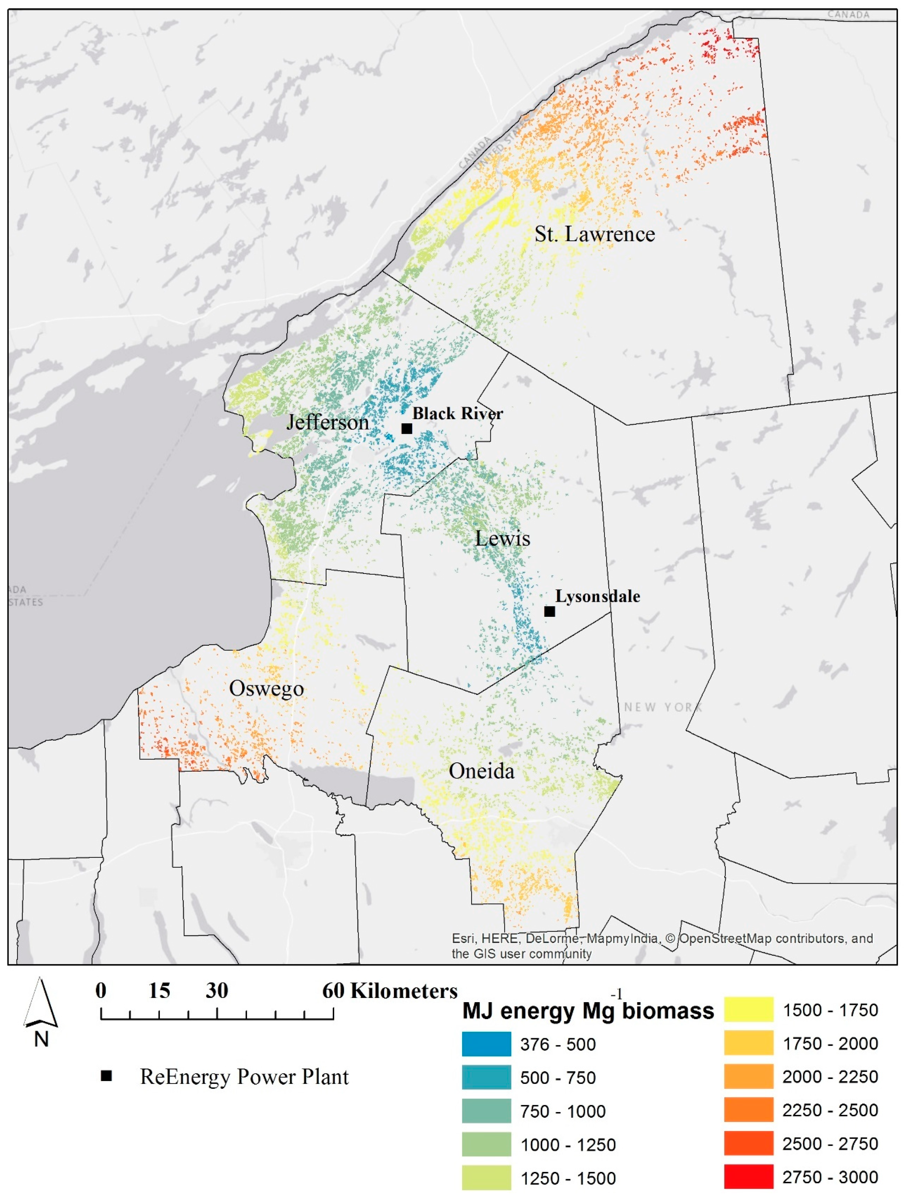
3.2. Spatial LCA Results across the Landscape

There are 9718 tax parcels (210,799 ha) suitable for growing willow in the five counties in central and northern NY (Table S2). Among these suitable parcels, pasture and cultivated cropland are the most common types and comprise the largest areas in all five counties, totaling 9018 parcels and occupying 88.7% or 186,870 ha of total suitable area. Among the five counties, Jefferson County and Oneida County showed the highest potential yield in pasture/cropland with a mean estimated yield of approximately 12.1 and 12.0 Mg ha−1 yr−1, respectively (Table S3). Lewis County and Oswego County have lower estimated yields on pasture/cropland with mean values of 10.8 and 11.3 Mg ha−1 yr−1, respectively. Within each county there are considerable variations of NCCPI values ranging from 0.03 to 0.96 in both grassland and cropland, reflecting various soil conditions, climate, water availability, and landscape values (Table S4). The estimated yield from NCCPI showed that cropland, i.e., pasture and cultivated crop in NLCD, on average has a 1 Mg ha−1 yr−1 higher yield of willow biomass than grassland, i.e., shrub and grassland in NLCD (Table S3) which still showed high potential with yields around 10 Mg ha−1 yr−1. These estimated numbers are consistent with measured yield numbers in recent trials in the area and with other modeled yield numbers for willow in the US [28,38,39].
The calculated production over seven rotations show a large variation among parcels (Figure 4) across the five counties (Figure 5), reflecting various environmental factors. A large number of parcels with high potential for biomass production are located in southwest and northeast Jefferson County with yield estimates greater than 14 Mg ha−1 yr−1 and relatively short distances to the Black River power plant. In addition, parcels in the southern parts of Oswego County and Oneida County, and the eastern parts of St. Lawrence County show relatively high yield estimates larger than 12 Mg ha−1 yr−1. However, the longer transportation distances in these areas can be limiting factors for biomass production, both in terms of GHG emissions and economics. In Lewis County, although yield estimates are around 10 Mg ha−1 yr−1 for many parcels, the shorter distances to end users are advantageous for efficient biomass production. In sum, it is advisable to consider yield potential for producing willow biomass because of variable conditions across geographical locations in the area.
The spatial nature of this LCA modeling process resulted in a broader range of items being included in the uncertainty analysis than has previously been done for willow biomass crops. The LCA model generated life cycle GHG emissions and energy consumption for each parcel using site-specific yield, land cover, SOC change rate, and transportation distance data across the five counties. There is considerable variation in the life cycle GHG emissions among land cover classes within each county. Parcels classified as cropland resulted in net-negative life cycle CO2 emissions, whereas most grassland parcels have net-positive CO2 emissions (Figure 6 and Figure 7), reflecting the different SOC changes of the two land cover categories. In the 30-cm grassland scenario in Jefferson county, one standard deviation is 28.2 kg CO2eq Mg−1, accounting for 57% of the mean value of 49.4 kg CO2eq Mg−1 in the county. The range is from −13.47 to 108.25 kg CO2eq Mg−1 in the county. In the 30-cm cropland scenario in St. Lawrence, one standard deviation is 37.57 kg CO2eq Mg−1, accounting for 71% of the mean −53.17 kg CO2eq Mg−1, and the life cycle GHG emissions range from 21.45 to −122.46 kg CO2eq Mg−1. Many parcels in Jefferson county that are close to an end user have large life cycle GHG emissions because they are classified as grassland and/or they have lower yield estimates (Figure S3).
The amount of uncertainty in energy consumption varied between counties and prior land uses (Figure 8 and Figure 9). Cropland parcels usually have lower energy consumption compared to other parcels due a higher yield and a lower energy investment in site preparation and management operations (Figure 8). The largest mean energy consumption, 2078 MJ Mg−1 biomass, is in the St. Lawrence grassland scenario and is more than double the energy input of the mean result in Lewis County (1002 MJ Mg−1 biomass). These correspond to an EROI of 8.95 in the St. Lawrence grassland scenario and 18.6 in Lewis County. This difference is mostly caused by transport distances to the end users in the two counties. Furthermore, the variations within individual counties are considerable. In the grassland scenario in Lewis County, the standard deviation is 198.7 MJ Mg−1, accounting for 19.8% of the 1002 MJ Mg−1 mean energy consumption in the county, and the number ranges from 515.5 to 1518 MJ Mg−1 (i.e., EROI from 36.08 to 12.26), almost a threefold increase. Similarly, for the cropland scenario in Lewis County, the standard deviation is 155.5 MJ compared to the mean of 910.4 MJ Mg−1 and the range of energy consumption values is from 538.9 to 1422 MJ Mg−1 (i.e., EROI from 34.51 to 13.08). This suggests that selection of where to grow willow crops within inside a county has an impact on both energy consumption and the EROI of the system.

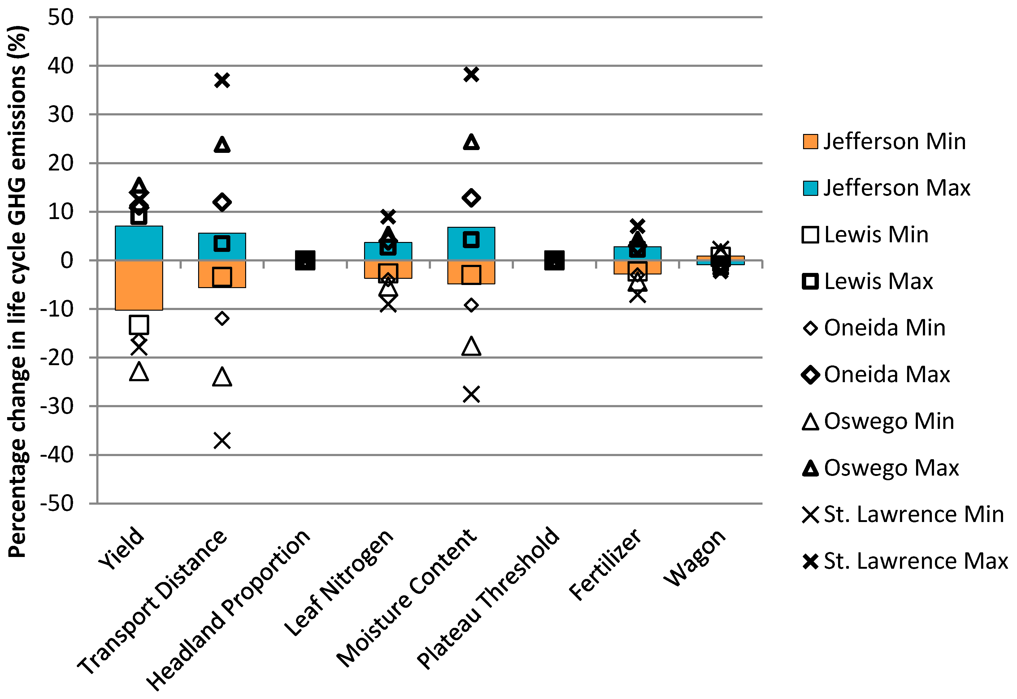
3.3. Sensitivity Analysis of Life Cycle GHG Emissions

The sensitivity analysis, conducted based on Table 1 parameters, shows that yield, transport distance, and moisture content of willow biomass are the most influential factors for the life cycle GHG emissions (Figure 10) in all counties in cropland with 30-cm soil depth. The response of life cycle GHG emissions to yield is counterintuitive, as increased yield caused higher net GHG emissions in the sensitivity analysis. This occurs because the change associated with the fixed increase in SOC being spread over more Mg is larger than the increase in belowground carbon that occurs when yield increases. The transportation distance and moisture content cause substantial variability in Oneida, Oswego, and St. Lawrence counties where baseline transportation distances are large. This result suggests that GHG emissions can be reduced by selecting fields close to end users, e.g., power plants.
The life cycle GHG emissions of parcels in all counties are related to the transportation distance, but they showed variability as well. Most pasture/cropland parcels cluster below zero net GHG emissions and have a clear increasing pattern with rising transportation distance (Figure 11). Similarly, shrub/grassland parcels cluster above zero net GHG emissions and are more scattered near smaller transportation distances due to relatively larger influences from other factors.

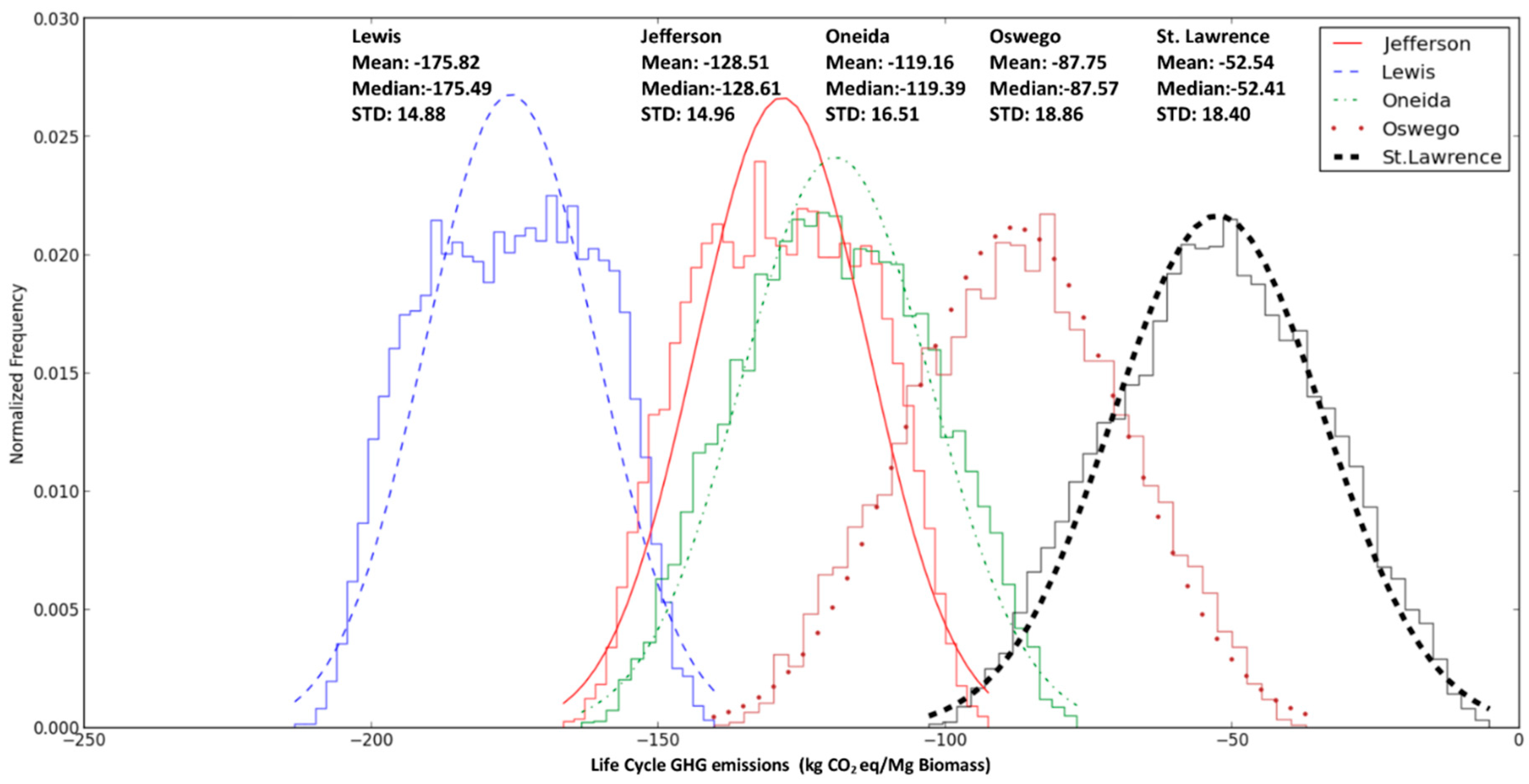
3.4. Uncertainty Analysis of Life Cycle GHG Emissions

To address the variability of GHG emissions in parcels despite the observed relation with transportation distance, Monte Carlo analyses of pasture and cropland in 30-cm soil were conducted. The distributions of life cycle GHG emissions in the five counties followed normal distributions (Figure 12) with different mean and standard deviations due to the uncertainty of varying SOC change rate, transport distance, yield, and other input parameters. The mean values of these distributions represent the life cycle GHG emissions values with the highest probability given the distributions of parameters in Table 1. Most counties have distinctive life cycle GHG emissions values, i.e., the chance of having the same values are very small or close to zero between Lewis County and Oswego County. However, a few counties, e.g., Jefferson and Oneida, have a higher probability of having similar life cycle GHG emissions values due to large overlaps of their probability distribution, although some of their parameters are very different, e.g., the baseline transport distance of Oneida County is twice that of Jefferson County.

4. Discussion

This study illustrates that willow crops are a biomass feedstock that is carbon-negative across the landscape when it is grown on land that was formerly in cropland/pasture, which makes up 88.6% of the suitable parcels identified (Table S3), and is a low-carbon feedstock when grown on grassland. When cropland/pasture is converted to willow, the baseline GHG emissions are −126.8 kg CO2eq Mg−1 biomass while the spatial analysis shows that some parcels have GHG emissions below −200 kg CO2eq Mg−1 biomass. The negative life cycle emissions for willow grown on cropland occur across almost all of the parcels in the five county regions, except for a couple of percent that are above 0 kg CO2eq Mg−1 when one way transportation distances exceed 126 km. When willow is grown on former grassland, which makes up 11.4% of the identified suitable parcels, the baseline life cycle GHG emissions are 27.7 kg CO2eq Mg−1 biomass and over 99% of all parcels are positive. The feedstock from these parcels can be considered a low carbon source of biomass. A previous LCA of willow grown in the region reported negative GHG emissions for all the scenarios, which included different transportation distances, high and low yields, and the application of N fertilizer or no fertilizer [1]. A review of LCAs in Europe and North America reported slightly positive GHG emissions (14–207 kg CO2eq Mg−1), but most of these studies excluded an assessment of belowground carbon and SOC changes associated with direct land use change [9]. Both these factors were included in this study using the best available, but limited, data and their influence on the results highlights a need for additional studies to refine this information. For willow grown on former cropland/pasture in this study there is the potential to sequester carbon while producing feedstock that can be used to provide a range of bioenergy and bioproducts and simultaneously create jobs and provide a range of other ecosystem services like improved water and soil quality and enhanced biodiversity [40].
The variations in life cycle GHG emissions between and within counties are substantial and driven by multiple parameters that have different resolutions ranging from the sub parcel (e.g., SSURGO at 10 m resolution) to county level (e.g., SOC change). For the cropland 30-cm soil scenarios, the GHG emissions differed by county ranging from −176.9 kg CO2eq Mg−1 in Lewis to −53.2 kg CO2eq Mg−1 in St. Lawrence. For the grassland 30-cm soil scenarios, Jefferson has the lowest mean GHG emissions: 49.4 kg CO2eq Mg−1 compared to 134.2 kg CO2eq Mg−1 in Oswego (Figure 7). Although Jefferson and Lewis counties are both close to the two end users, the life cycle GHG emissions for grassland in Lewis County had larger values due to higher rates of SOC change (Table 3) and lower yield (Table S3) than Jefferson County (49.4 kg CO2eq Mg−1). The transportation distance for Lewis County is generally much smaller than Oneida County, however, the life cycle GHG emissions of Oneida County in grassland are lower than Lewis County due to higher yields and a similar SOC change rate. The impact of transportation distances, yield estimates, which also impacted values for belowground biomass and harvesting operations, and changes in SOC on GHG emissions varied parcel to parcel in this study, creating complex patterns across the landscape (Figure 7). Using LCA and other tools that use a systems approach to analysis and create a framework for examining the interactions among different components is important to understand the overall GHG emissions from these systems and the factors that need to be addressed to further improve and reduce uncertainty for willow systems.
The net-positive life cycle GHG emissions from grassland compared to the negative net emissions for cropland are largely due to the different modeled changes in SOC associated with land use change. The baseline results use an average SOC change rate across the five counties of 0.28 Mg carbon ha−1 yr−1 (ranging from 0.19 to 0.34 Mg carbon ha−1 yr−1) sequestration rate for 30-cm soil in cropland/pasture and −0.29 Mg carbon ha−1 yr−1 change rate (ranging from −0.19 to −0.43 Mg carbon ha−1 yr−1) (Table 3) in hay/grasslands after conversion to willow crops [19]. The SOC change rate in 100-cm soil is higher than that in 30-cm soil, because the SOC modeling of 100-cm simulates both topsoil (0–30cm) and subsoil (30–100cm) including additional soil organic matter pool for the subsoil [19]. However, the majority of willow in northern NY is growing on marginal land and the soil depth is often limited due to perched water tables, hardpans, or bedrock. Previous assessments of rooting depth in willow in the region limited sampling to 45 cm because soil conditions limited root development in almost all cases [17]. Thus, while SOC changes are reported here to 100 cm depth, the number of sites where willow will be grown in this region and changes will occur to this depth are probably limited. Incorporating the best available data on soil carbon change due to land use change for a willow energy crop into a spatial LCA is an important step forward in the understanding of these systems, but the data is only available on the county level and does not capture the range of variation across the landscape. The results of this study emphasize the importance of this change in the overall GHG balance of these systems and that better data on these changes are needed. For example, SSURGO soil data is at spatial scale of 10 m, and potential future improvement of current county-level SOC data from CENTURY would support more detailed parcel-level soil SOC modeling from LUC including soil variations at the parcel level.
We incorporated SOC change associated with direct land use change in this study because of the impact it has on the results for willow biomass as well as biofuels that are produced from this material [41]. The baseline GHG emissions in this study (30 cm depth) without SOC change was −52.3 kg CO2eq Mg−1 for cropland and −49.9 kg CO2eq Mg−1 for grassland, which were similar to the −52.7 kg CO2eq Mg−1 value for the high yield-fertilized-long transportation distance scenario reported in an earlier study [1]. When SOC change is included, the baseline values in this study become −126.8 kg CO2eq Mg−1 for cropland and 27.7 CO2eq Mg−1 for grassland. For both grassland and cropland, SOC change is the second largest factor, after belowground carbon, contributing to the overall life cycle GHG emissions. Caputo et al. (2013) included belowground biomass but not SOC changes and had negative GHG emissions in all their scenarios [1]. Few of the studies reviewed by Djomo et al. (2011) included changes in soil carbon or belowground carbon stored in coarse roots and stools, and the GHG impact of these studies were all positive, ranging from 0.7 to 10.6 g CO2eq MJ−1 (13.7–208.8 kg CO2eq Mg−1) [9]. The inclusion of the SOC and belowground carbon included in this study results in negative GHG emissions for cropland and slightly positive values for grassland that are at the low end of the range reported by Djomo et al. (2011) [9]. In a more recent LCA that included soil carbon sequestration [42], the life cycle GHG emissions of willow biomass production were estimated as 0.8 g CO2eq MJ−1 for arable land, −10.4 g CO2eq MJ−1 for marginal pastureland, and −31.8 g CO2eq MJ−1 for marginal abandoned land in 100-cm soil depth. For the three scenarios there were changes in SOC (28.5 kg C ha−1 yr−1 for arable land, SOC gain of 153.4 kg C ha−1 yr−1 for marginal pastureland, and SOC loss of 31.5 kg C ha−1 yr−1 for marginal abandoned land) in contrast to the SOC increases in cropland but decreases in grassland used in this study. However, the differences of life cycle GHG emissions by SOC change were relatively minor compared to other processes such as transportation [42]. The inclusion of changes in SOC carbon associated with land use change is important to understand the impacts and benefits of these systems, but better data is needed to understand these patterns.
There is a limited amount of data available on changes in SOC under willow, especially in North America, and the results are inconclusive. A meta-analysis showed that a transition from cropland to short rotation coppice willow or poplar increased SOC by 5.0% ± 7.8% and by 3.7% ± 14.6% when these crops were planted on grassland [43]. These analyses only had 18 data points for cropland and seven for grassland, so there is large amount of uncertainty. An earlier analysis suggested an increase in SOC over time when poplar or willow are planted on cropland and no change or a slight decrease when planted on grassland, but model results vary based on the time period of the assessment [20,21]. For example, losses of 7–8% of soil C were suggested for data collected in the first 5 years after willow is planted on grassland, but for studies that had time frames longer than 5 years there is no significant change from the baseline [20,21]. A side by side study of willow and grassland over a 2-year period showed that willow was a net carbon sink even when biomass was harvested while the grassland was a net source of carbon [44]. This study is limited to one site and, as is the case with all studies, is influenced by site and management practices both before and during the study. A soil C chronosequence study, ranging from 5 to 19 years old, for willow in the region of the US where this study occurs suggests little change over that time period [19]. The data on SOC changes associated with willow biomass crops is limited and uncertain. We used the best available data based on SOC change associated with direct land use change based on modeling done by the Argonne National Lab using the CENTURY model, but this data was only available at the county level. More information on the dynamics of direct land use change for woody crops as well as a better understanding of long-term change in soil C are needed to reduce uncertainty and the overall GHG balance of willow systems across the landscape.
The inclusion of belowground biomass in this and other studies is important because of the magnitude of its impact. In this study, it is the largest single carbon sink, but as is the case with SOC data, information on this important component of the system is limited. In the 30-cm soil grassland scenario, belowground carbon accounts for −144.71 kg CO2eq Mg−1 (45.6% of the total impacts in absolute numbers) and the SOC change accounts for 77.55 kg CO2eq Mg−1 (24.5% of the total impacts). One study in the US of the carbon stored in belowground biomass suggests it changes over several rotations and is substantial, 45.3 ± 4.4 Mg CO2eq ha−1 (25.4 Mg C ha−1) [32]. This is 1.6 to almost 3 times greater than the increase in soil carbon in willow relative to cropland and exceeded the losses in SOC replacing grassland. In another recent study, root:shoot ratios varied among cultivars (0.46–0.72) at one site but not at a second site (0.63–0.65) [31] but some of these differences were reduced when yields were used as a covariate in the analysis. The belowground biomass values used in this study are proportional to the aboveground biomass [31]; therefore, increasing the yield of stem biomass in turn increases belowground carbon sequestration. This allowed us to apply these belowground values on a parcel by parcel basis across the landscape, but there is a need for more detailed information on how the belowground portion of these system changes across sites and with different cultivars and management systems.
Aboveground biomass yield is the most widely studied aspect of SRWC because it is the main product generated from these systems. In this study, changes in yield across the landscape had a direct impact on belowground biomass values, throughput of the harvester, and influenced the impact of changes in SOC, which was a fixed value per ha for grassland or cropland across an entire county. By using the relationship between NCCPI and yield from a previous study, we were able to assign yield at the sub parcel level because NCCPI data is available at a 10 m resolution and the land cover data we used was available at 30 m. This data effectively represented yields that have been measured in research and commercial scale trials across the region. Recently developed models used to predict yield across the continental US used 800 m grid (64 ha) for climate data and a 1024 ha parcel size for soils data [38]. Using this model to predict yields in this study would have further limited our ability to assess changes across the landscape.
While transportation distance from the field to the gate of the end use facility has been noted as an important factor in the GHG emissions of willow and other energy crops in the past, this current spatial LCA analysis illustrates the importance of understanding how transportation distance interacts with other factors. In Caputo et al. (2014), there are two haul distance scenarios to biorefineries, namely long haul distance and short haul distance [1]. The baseline case in this study is similar to the short haul distance scenario in Caputo et al. (2014) with an average 35.5 km to biorefineries. The life cycle GHG emissions result of −126.8 kg CO2eq Mg−1 biomass in this study is at the lower end of the GHG emissions range from −83.1 to −138.3 CO2eq Mg−1 of short haul distances scenarios in Caputo et al. (2014) [1]. Sensitivity analyses in recent LCA studies of willow biomass crops in Sweden [14] and in Spain [45] showed that transportation distance had the largest influence on life cycle GHG emissions. In this study, transportation was consistently one of the top three factors influencing GHG emissions, but its impact was modified by other factors. For example, sensitivity analysis showed that transportation distances changed GHG emissions less than 5% in Jefferson county but by more than 10% for Oneida county. However, the resulting distribution of GHG emissions for Jefferson and Oneida county in the uncertainty analysis are similar because of other factors such as modeled SOC increases on cropland, which were 30% higher in Oneida than in Jefferson. Integrating multiple factors in a spatial LCA provides valuable information to support decision making on where to establish willow biomass crops if one of the goals is to minimize GHG emissions.
Harvesting accounts for 9.48 kg CO2eq Mg−1 in all scenarios and is the second largest impact among crop management activities after fertilizer, so improvements in harvester efficiency can contribute to GHG emission reductions. This number is about 27% lower than the 13 kg CO2eq Mg−1 value in a previous study [1] due to improvements in harvester efficiency of single pass cut and chip operations modeled in this study and improved data for harvester operation and fuel consumption that have been made over the past few years [29,46]. Site management is an integrated category including all site preparation, planting, and site maintenance processes, specifically including processes #1 to # 15 and process #20 in Table S1. Site management activities are a small component of the total life cycle GHG emissions because they only occur once in the 25-year time span of this system, accounting for 4.40 kg CO2eq Mg−1 in 30 cm grassland scenarios and are slightly lower for cropland (1.97 kg CO2eq Mg−1) scenarios because fewer site preparation operations are required.
Willow biomass has a high energy ratio in central and northern New York State; the energy consumption was estimated as 969.6 MJ for 1 Mg biomass, and the net EROI is 19.2. For cropland, this number dropped to 937.9 MJ for 1 Mg biomass and increased to 19.8 as EROI. The overall GHG impact and energy balance of an energy system will depend on the conversion technology and final end products generated from the willow biomass.
The energy consumption values are mainly affected by transportation distance to the end users (Black River and Lyonsdale). The parcels near the power plants show less than 500 MJ Mg−1 energy consumption compared with over 2750 MJ Mg−1 in energy consumption in parcels further away (Figure 9). The geographical distributions of energy consumption demonstrate that parcels further away from end users tend to have higher energy input largely due to increasing the transportation distance. However, the pattern of increasing energy consumption is not strictly circular centering around the end users because it is also impacted by the spatial distribution of yield and land cover types and the tortuosity of the roads in portions of the study region.
Harvesting and fertilization are the two largest energy inputs to willow biomass production, which agrees with other studies [1,9,14]. These management activities contribute 14% (harvesting) and 17% (fertilization) of the total energy consumption of 969.6 MJ Mg−1 for the baseline grassland scenario. The energy demand of willow biomass production in Caputo et al. (2014) ranges from 445.0 to 1052.4 MJ Mg−1 biomass for eight scenarios with variations in transportation distance, yield, and fertilizer application [1]. Energy inputs in this study are larger than six of the eight scenarios in Caputo et al. (2014), with the four lowest energy inputs being scenarios that exclude fertilizer inputs and the associated input of 164.6 MJ Mg−1. Another difference is the inclusion in this study of a process to load chips from piles on the ground into trucks for delivery to an end user, which is the most common practice in the region. In this study, the energy input associated with loading chips was about 35% higher than site management energy inputs for grassland and 2.8 times greater for the cropland scenario because it is an activity that occurs multiple times over the life of the crop. As a result, the range of EROI values in this study (8.95 in the St. Lawrence grassland scenario to 18.6 in the Lewis county cropland scenario) is on the lower end compared to the range of EROIs of 18.3 to 43.4 in Caputo et al. (2014) [1]. However, this study’s EROI values are at the high end of the 3–16 values for cradle-to-plant LCA studies reviewed in Djomo et al. (2011) [9]. Harvesting throughput values in our study are based on more recent data that showed a substantial improvement in harvester throughput [29,46] that results in lower energy consumption per Mg of biomass and a higher EROI. Further improvements in harvesting and chip loading operations may be possible to further lower energy inputs into the system.
One approach to increase EROI in this system, and reduce GHG emissions, is to replace synthetic fertilizer with organic amendments or eliminate fertilizer applications, as long as the yield can be maintained. However, the yield response of willow to different rates of fertilizer is not well defined with most previous studies in the region (except for Adegbidi et al. (2001) [47]) showing no statistical improvement in yield with fertilizer additions [48,49]. However, a recent meta data analysis of willow fertilization trials across North America and Europe indicated that there was a lot of variation in yield response, but an overall positive trend was present [50]. Another option to shift fossil fuels based fertilizer energy inputs is to use organic waste materials like manure or biosolids, which Heller et al. (2003) suggested could increase EROI by 33–45% [51]. Regional studies showed that these materials produce yields comparable to commercial fertilizer [49,52]. While we included a range of fertilizer additions in the sensitivity analysis of this study, we did not include an associated change in yield because of the uncertainty of this relationship. Being able to further define the yield response to fertilizer additions across a range of soil types and site conditions would allow a better assessment of the impact of fertilizer on EROI and GHG emissions in willow systems.

5. Conclusions

Knowledge of how GHG emissions and energy ratios of willow biomass crops change across the landscape is useful information when evaluating the benefits and impacts of this system and an associated conversion facility. This study provides insights about how land cover, transportation distance, and yield vary among parcels where willow can be grown and how they interact to result in various life cycle GHG emissions and energy ratios. Across the vast majority of the region cropland/pasture converted to willow sequestered carbon until the haul distance was greater than 125 km regardless of other parameters such as yield. Key variables contributing to this result are the projected increase in SOC when willow is planted on cropland and the accumulation of carbon in the below ground portions of the willow plants. Grassland that was converted to willow almost always had slightly positive life cycle GHG emissions based on the projected increase in SOC. The importance of SOC change and belowground carbon indicates that more precise and accurate data on these parameters is needed to refine these results in order to more completely understand patterns across the landscape.
Energy inputs needed to produce one Mg of willow biomass crops were largely dependent on the transportation distance to the end users. The haul distance from the willow crop to the end user has continually been shown to be a key factor related to energy use, but it is one that is not easily changed until renewable biodiesel or electric power become common for tractor trailers. Other changes that can be made to the system to reduce energy inputs include replacing synthetic fertilizer with organic amendments or not applying fertilizer altogether as long as yields are maintained, and improving the efficiency of the harvesting system.
Sensitivity analysis of the life cycle GHG emissions for the five counties showed that yield, transportation distance, moisture content of biomass, and fertilizer use are among the most critical parameters that contribute to the overall GHG emissions of willow biomass across five counties. The moisture content of the biomass impacts the GHG emissions associated with transportation but is a factor that has some potential to be managed. The Monte Carlo uncertainty analysis showed that with the shorter haul distances in Lewis County, the most likely GHG emissions are around −175 kg CO2eq per Mg, whereas in areas with long distances, like St. Lawrence county, emissions are less negative (−50 kg CO2eq per Mg). The probabilities and ranges of GHG emission values in the five counties can be estimated based on the resulting normal distribution curves, providing informative guidelines for land managers, policy makers, and scientists.

Supplementary Materials

The Supporting Information document containing Tables S1–S4 and Figures S1–S4 is available online at https://www.mdpi.com/1996-1073/13/16/4251/s1.

Author Contributions

Conceptualization, S.Y., T.A.V., and M.-O.P.F.; methodology, S.Y., M.-O.P.F., and T.A.V.; software, S.Y. and M.-O.P.F.; validation, S.Y. and T.A.V.; formal analysis, S.Y.; investigation, S.Y.; resources, S.Y., T.A.V., and M.-O.P.F.; data curation, S.Y. and T.A.V.; writing—original draft preparation, S.Y.; writing—review and editing, T.A.V., M.-O.P.F., and S.Y.; visualization, S.Y.; supervision, T.A.V.; project administration, T.A.V.; funding acquisition, T.A.V. All authors have read and agreed to the published version of the manuscript.

Funding

This research was funded by the US Department of Energy Bioenergy Technologies Office, grant number DE-EE0006638; the New York State Energy Research and Development Authority (NYSERDA), grant number 30713; and an Agriculture and Food Research Initiative competitive grant from the US Department of Agriculture (USDA) National Institute of Food and Agriculture, grant number 2012-68005-19703.

Acknowledgments

The authors thank the reviewers for their comments.

Conflicts of Interest

The authors declare no conflict of interest. The funders had no role in the design of the study; in the collection, analyses, or interpretation of data; in the writing of the manuscript, or in the decision to publish the results.

References

  1. Caputo, J.; Balogh, S.B.; Volk, T.A.; Johnson, L.; Puettmann, M.; Lippke, B.; Oneil, E. Incorporating uncertainty into a life cycle assessment (LCA) model of short-rotation willow biomass (Salix spp.) crops. Bioenergy Res. 2014, 7, 48–59. [Google Scholar] [CrossRef]
  2. Rowe, R.L.; Street, N.R.; Taylor, G. Identifying potential environmental impacts of large-scale deployment of dedicated bioenergy crops in the UK. Renew. Sustain. Energy Rev. 2009, 13, 271–290. [Google Scholar] [CrossRef]
  3. Braun, R.; Karlen, D.; Johnson, D. Sustainable alternative fuel feedstock opportunities, challenges and roadmaps for six US regions. In Proceedings of the Sustainable Feedstocks for Advanced Biofuels Workshop, Atlanta, GA, USA, 28–30 September 2010; pp. 28–30. [Google Scholar]
  4. Volk, T.A.; Verwijst, T.; Tharakan, P.J.; Abrahamson, L.P.; White, E.H. Growing fuel: A sustainability assessment of willow biomass crops. Front. Ecol. Environ. 2004, 2, 411–418. [Google Scholar] [CrossRef]
  5. Langholtz, M.; Stokes, B.; Eaton, L. 2016 Billion-Ton Report: Advancing Domestic Resources for a Thriving Bioeconomy, Volume 1: Economic Availability of Feedstock; Oak Ridge National Laboratory: Oak Ridge, TN, USA, 2016; 411p. [Google Scholar]
  6. New York State Climate Action Council. Climate Leadership and Community Protection Act (Climate Act); New York State Climate Action Council: Albany, NY, USA, 2019. [Google Scholar]
  7. New York State Public Service Commission. New York’s Clean Energy Standard; New York State Public Service Commission: New York, NY, USA, 2015.
  8. McBride, A.C.; Dale, V.H.; Baskaran, L.M.; Downing, M.E.; Eaton, L.M.; Efroymson, R.A.; Garten, C.T., Jr.; Kline, K.L.; Jager, H.I.; Mulholland, P.J. Indicators to support environmental sustainability of bioenergy systems. Ecol. Indic. 2011, 11, 1277–1289. [Google Scholar] [CrossRef]
  9. Djomo, S.N.; KASMIOUI, O.E.; Ceulemans, R. Energy and greenhouse gas balance of bioenergy production from poplar and willow: A review. GCB Bioenergy 2011, 3, 181–197. [Google Scholar] [CrossRef]
  10. Buonocore, E.; Franzese, P.P.; Ulgiati, S. Assessing the environmental performance and sustainability of bioenergy production in Sweden: A life cycle assessment perspective. Energy 2012, 37, 69–78. [Google Scholar] [CrossRef]
  11. Murphy, F.; Devlin, G.; McDonnell, K. Energy requirements and environmental impacts associated with the production of short rotation willow (Salix sp.) chip in Ireland. GCB Bioenergy 2014, 6, 727–739. [Google Scholar] [CrossRef] [Green Version]
  12. Yoshioka, T.; Inoue, K.; Hartsough, B. Cost and Greenhouse Gas (GHG) Emission Analysis of a Growing, Harvesting, and Utilizing System for Willow Trees Aimed at Short Rotation Forestry (SRF) in Japan. J. Jpn. Inst. Energy 2015, 94, 576–581. [Google Scholar] [CrossRef] [Green Version]
  13. Hammar, T.; Ericsson, N.; Sundberg, C.; Hansson, P.-A. Climate impact of willow grown for bioenergy in Sweden. BioEnergy Res. 2014, 7, 1529–1540. [Google Scholar] [CrossRef] [Green Version]
  14. Hammar, T.; Hansson, P.A.; Sundberg, C. Climate impact assessment of willow energy from a landscape perspective: A Swedish case study. GCB Bioenergy 2017, 9, 973–985. [Google Scholar] [CrossRef] [Green Version]
  15. Styles, D.; Börjesson, P.; d’Hertefeldt, T.; Birkhofer, K.; Dauber, J.; Adams, P.; Patil, S.; Pagella, T.; Pettersson, L.B.; Peck, P. Climate regulation, energy provisioning and water purification: Quantifying ecosystem service delivery of bioenergy willow grown on riparian buffer zones using life cycle assessment. Ambio 2016, 45, 872–884. [Google Scholar] [CrossRef] [PubMed] [Green Version]
  16. Bacenetti, J.; Bergante, S.; Facciotto, G.; Fiala, M. Woody biofuel production from short rotation coppice in Italy: Environmental-impact assessment of different species and crop management. Biomass Bioenergy 2016, 94, 209–219. [Google Scholar] [CrossRef]
  17. Krzyżaniak, M.; Stolarski, M.; Szczukowski, S.; Tworkowski, J. Life cycle assessment of new willow cultivars grown as feedstock for integrated biorefineries. BioEnergy Res. 2016, 9, 224–238. [Google Scholar] [CrossRef] [Green Version]
  18. Pacaldo, R.S.; Volk, T.A.; Briggs, R.D. Carbon sequestration in fine roots and foliage biomass offsets soil CO 2 effluxes along a 19-year chronosequence of shrub willow (Salix x dasyclados) biomass crops. Bioenergy Res. 2014, 7, 769–776. [Google Scholar] [CrossRef]
  19. Pacaldo, R.S.; Volk, T.A.; Briggs, R.D. No significant differences in soil organic carbon contents along a chronosequence of shrub willow biomass crop fields. Biomass Bioenergy 2013, 58, 136–142. [Google Scholar] [CrossRef]
  20. Qin, Z.; Dunn, J.B.; Kwon, H.; Mueller, S.; Wander, M.M. Soil carbon sequestration and land use change associated with biofuel production: Empirical evidence. GCB Bioenergy 2016, 8, 66–80. [Google Scholar] [CrossRef] [Green Version]
  21. Qin, Z.; Dunn, J.B.; Kwon, H.; Mueller, S.; Wander, M.M. Influence of spatially dependent, modeled soil carbon emission factors on life-cycle greenhouse gas emissions of corn and cellulosic ethanol. GCB Bioenergy 2016, 8, 1136–1149. [Google Scholar] [CrossRef]
  22. Krzyzaniak, M.; Stolarski, M.; Szczukowski, S.; Tworkowski, J. Life cycle assessment of willow produced in short rotation coppices for energy purposes. J. Biobased Mater. Bioenergy 2013, 7, 566–578. [Google Scholar] [CrossRef]
  23. Whittaker, C.; Macalpine, W.; Yates, N.E.; Shield, I. Dry Matter Losses and Methane Emissions During Wood Chip Storage: The Impact on Full Life Cycle Greenhouse Gas Savings of Short Rotation Coppice Willow for Heat. BioEnergy Res. 2016, 9, 820–835. [Google Scholar] [CrossRef] [Green Version]
  24. González-García, S.; Mola-Yudego, B.; Dimitriou, I.; Aronsson, P.; Murphy, R. Environmental assessment of energy production based on long term commercial willow plantations in Sweden. Sci. Total Environ. 2012, 421, 210–219. [Google Scholar] [CrossRef]
  25. Eisenbies, M.H.; Volk, T.A.; Espinoza, J.; Gantz, C.; Himes, A.; Posselius, J.; Shuren, R.; Stanton, B.; Summers, B. Biomass spacing and planting design infleunce cut-and-chip harvesting of hybrid poplar. Biomass Bioenergy 2017, 106, 182–190. [Google Scholar] [CrossRef]
  26. Bush, C.; Volk, T.A.; Eisenbies, M.H. Planting rates and delays during the establishment of willow biomass crops. Biomass Bioenergy 2015, 83, 290–296. [Google Scholar] [CrossRef]
  27. Eisenbies, M.H.; Volk, T.A.; Patel, A. Changes in feedstock quality in willow chip piles created in winter from a commercial scale harvest. Biomass Bioenergy 2016, 86, 180–190. [Google Scholar] [CrossRef] [Green Version]
  28. Sleight, N.J.; Volk, T.A. Recently bred willow (Salix spp.) biomass crops show stable yield trends over three rotations at two sites. BioEnergy Res. 2016, 9, 782–797. [Google Scholar] [CrossRef]
  29. Eisenbies, M.H.; Volk, T.A.; Posselius, J.; Foster, C.; Shi, S.; Karapetyan, S. Evaluation of a single-pass, cut and chip harvest system on commercial-scale, short-rotation shrub willow biomass crops. Bioenergy Res. 2014, 7, 1506–1518. [Google Scholar] [CrossRef]
  30. De Klein, C.; Novoa, R.S.; Ogle, S.; Smith, K.A.; Rochette, P.; Wirth, T.C.; McConkey, B.G.; Mosier, A.; Rypdal, K.; Walsh, M. N2O emissions from managed soils, and CO2 emissions from lime and urea application. In IPCC Guidelines for National Greenhouse Gas Inventories; Institute for Global Environmental Strategies: Kanagawa, Japan, 2006. [Google Scholar]
  31. Sleight, N.; Volk, T.; Fandrich, K.; Eisenbies, M. Above- and belowground biomass of willow cultivars: Quantities, Distribution and Carbon Storage. In Proceedings of the NewBio Annual Meeting, Morgantown, WV, USA, 3–5 August 2015. [Google Scholar]
  32. Pacaldo, R.S.; Volk, T.A.; Briggs, R.D. Greenhouse gas potentials of shrub willow biomass crops based on below-and aboveground biomass inventory along a 19-year chronosequence. BioEnergy Res. 2013, 6, 252–262. [Google Scholar] [CrossRef]
  33. Dunn, J.B.; Mueller, S.; Qin, Z.; Wang, M. Carbon Calculator for Land Use Change from Biofuels Production (CCLUB 2015); ANL/ESD/12-5 Rev. 3; Argonne National Laboratory: Lemont, IL, USA; U.S. Department of Energy: Oak Ridge, TN, USA, 2014.
  34. Homer, C.G.; Dewitz, J.A.; Yang, L.; Jin, S.; Danielson, P.; Xian, G.; Coulston, J.; Herold, N.D.; Wickham, J.D.; Megown, K. National Land Cover Database 2011 (NLCD 2011); United States Geological Survey, Ed.; Multi-Resolution Land Characteristics Consortium (MRLC): Sioux Falls, SD, USA, 2015.
  35. Wickham, J.; Stehman, S.V.; Gass, L.; Dewitz, J.A.; Sorenson, D.G.; Granneman, B.J.; Poss, R.V.; Baer, L.A. Thematic accuracy assessment of the 2011 national land cover database (NLCD). Remote Sens. Environ. 2017, 191, 328–341. [Google Scholar] [CrossRef] [Green Version]
  36. Castellano, P.; Volk, T.; Herrington, L. Estimates of technically available woody biomass feedstock from natural forests and willow biomass crops for two locations in New York State. Biomass Bioenergy 2009, 33, 393–406. [Google Scholar] [CrossRef]
  37. New York State Energy Research & Development Authority. Renewable Fuels Roadmap and Sustainable Biomass Feedstock Supply for New York: Appendix E. Available online: https://www.nyserda.ny.gov/About/Publications/Research-and-Development-Technical-Reports/Biomass-Reports/Renewable-Fuels-Roadmap (accessed on 12 August 2020).
  38. Volk, T.A.; Berguson, B.; Daly, C.; Halbleib, M.D.; Miller, R.; Rials, T.G.; Abrahamson, L.P.; Buchman, D.; Buford, M.; Cunningham, M.W. Poplar and shrub willow energy crops in the United States: Field trial results from the multiyear regional feedstock partnership and yield potential maps based on the PRISM-ELM model. GCB Bioenergy 2018, 10, 735–751. [Google Scholar] [CrossRef]
  39. Johnson, G.; Volk, T.; Hallen, K.; Shi, S.; Bickell, M.; Heavey, J. Shrub willow biomass production ranking across three harvests in New York and Minnesota. BioEnergy Res. 2018, 11, 305–315. [Google Scholar] [CrossRef]
  40. Volk, T.A.; Heavey, J.P.; Eisenbies, M.H. Advances in shrub-willow crops for bioenergy, renewable products, and environmental benefits. Food Energy Secur. 2016, 5, 97–106. [Google Scholar] [CrossRef] [Green Version]
  41. Therasme, O.; Volk, T.A.; Fortier, M.-O.P.; Eisenbies, M.H.; Amidon, T.E. Climate benefits of biofuel from shrub willow hot water extraction process in the northeast United States. Biotechnol. Biofuels 2020. under review. [Google Scholar]
  42. Saez de Bikuña, K.; Hauschild, M.Z.; Pilegaard, K.; Ibrom, A. Environmental performance of gasified willow from different lands including land-use changes. GCB Bioenergy 2017, 9, 756–769. [Google Scholar] [CrossRef] [Green Version]
  43. Harris, Z.; Spake, R.; Taylor, G. Land use change to bioenergy: A meta-analysis of soil carbon and GHG emissions. Biomass Bioenergy 2015, 82, 27–39. [Google Scholar] [CrossRef] [Green Version]
  44. Harris, Z.M.; Alberti, G.; Viger, M.; Jenkins, J.R.; Rowe, R.; McNamara, N.P.; Taylor, G. Land-use change to bioenergy: Grassland to short rotation coppice willow has an improved carbon balance. GCB Bioenergy 2017, 9, 469–484. [Google Scholar] [CrossRef]
  45. Gasol, C.M.; Gabarrell, X.; Rigola, M.; González-García, S.; Rieradevall, J. Environmental assessment: (LCA) and spatial modelling (GIS) of energy crop implementation on local scale. Biomass Bioenergy 2011, 35, 2975–2985. [Google Scholar] [CrossRef]
  46. Eisenbies, M.H.; Volk, T.A.; de Souza, D.P.; Hallen, K.W. Cut-and-chip harvester material capacity and fuel performance on commercial-scale willow fields for varying ground and crop conditions. GCB Bioenergy 2020, 12, 380–395. [Google Scholar] [CrossRef] [Green Version]
  47. Adegbidi, H.G.; Volk, T.A.; White, E.H.; Abrahamson, L.P.; Briggs, R.D.; Bickelhaupt, D.H. Biomass and nutrient removal by willow clones in experimental bioenergy plantations in New York State. Biomass Bioenergy 2001, 20, 399–411. [Google Scholar] [CrossRef]
  48. Stoof, C.R.; Richards, B.K.; Woodbury, P.B.; Fabio, E.S.; Brumbach, A.R.; Cherney, J.; Das, S.; Geohring, L.; Hansen, J.; Hornesky, J. Untapped potential: Opportunities and challenges for sustainable bioenergy production from marginal lands in the Northeast USA. BioEnergy Res. 2015, 8, 482–501. [Google Scholar] [CrossRef]
  49. Quaye, A.K.; Volk, T.A. Biomass production and soil nutrients in organic and inorganic fertilized willow biomass production systems. Biomass Bioenergy 2013, 57, 113–125. [Google Scholar] [CrossRef]
  50. Fabio, E.S.; Smart, L.B. Effects of nitrogen fertilization in shrub willow short rotation coppice production–a quantitative review. GCB Bioenergy 2018, 10, 548–564. [Google Scholar] [CrossRef]
  51. Heller, M.C.; Keoleian, G.A.; Volk, T.A. Life cycle assessment of a willow bioenergy cropping system. Biomass Bioenergy 2003, 25, 147–165. [Google Scholar] [CrossRef]
  52. Quaye, A.K.; Volk, T.A.; Hafner, S.; Leopold, D.J.; Schirmer, C. Impacts of paper sludge and manure on soil and biomass production of willow. Biomass Bioenergy 2011, 35, 2796–2806. [Google Scholar] [CrossRef]
Figure 1. System diagram of willow production supply chain with boundaries and major processes affecting greenhouse gas (GHG) emissions and energy consumption. Site preparation and planting processes occur once in the lifetime of the willow crop.
Energies 13 04251 g001
Figure 2. Five counties in central and northern New York State (Jefferson, Lewis, Oneida, Oswego, and St. Lawrence) where the spatial life cycle assessment (LCA) was conducted. The two power plants that have used willow as a portion of their fuel source shown as squares, Black River and Lyonsdale are owned by ReEnergy. Only primary roads are shown in the figure.
Energies 13 04251 g002
Figure 3. Life cycle GHG emissions from producing and delivering 1 Mg biomass represented by the yellow bar in four scenarios including 30 and 100 cm soil depths with grassland and cropland land cover converted to willow. The legend is read from left to right starting with site management as the first positive category, followed by fertilizer through to leaf decay.
Energies 13 04251 g003
Figure 4. Distribution of yield estimates over seven rotations based on National Commodity Crop Productivity Index (NCCPI) indices from the Soil Survey Geographical Database (SSURGO) soil data layer for parcels in five counties. The lines in boxes are 25th percentile, median, and 75th percentile. The cross markers represent mean values. The whiskers are minimum and maximum values.
Energies 13 04251 g004
Figure 5. Yield estimates in parcels suitable for willow biomass crops in five counties in central and northern New York. Yields are estimated based on average NCCPI values of each parcel from SSURGO soil data layer.
Energies 13 04251 g005
Figure 6. Boxplots showing distributions of willow biomass crop life cycle GHG emissions from parcel level LCA results in five counties in upstate NY. The upper bound, the notch, and lower bound represent 75th percentile, median, and 25th percentile, respectively. The green triangle indicates the mean.
Energies 13 04251 g006
Figure 7. Life cycle willow GHG emissions measured in kg CO2eq of producing 1 Mg dry biomass with SOC changes modeled for a 30 cm depth in suitable parcels in five counties. The high levels of CO2 sequestration (in blue) occur mostly near the end use facilities (Black River and Lyonsdale).
Energies 13 04251 g007
Figure 8. Boxplots of energy consumption to produce 1 Mg of willow biomass from parcel level LCA in five counties in central and northern NY. The upper and lower bounds of boxplots represent 75% and 25% quantiles, respectively. The notches represent median values and the triangles represent mean. For each county, the energy consumption is shown separately for grassland and cropland due to differences in yield and site preparation steps for the two land cover classes.
Energies 13 04251 g008
Figure 9. Energy consumption to produce 1 Mg willow biomass in the five counties in Central and Northern New York based on parcel-level LCA modeling.
Energies 13 04251 g009
Figure 10. Range of life cycle GHG emissions expressed as the percentage of the baseline life cycle GHG emissions by varying each parameter individually in sensitivity analysis to its minimum (“Min”) or maximum (“Max”) value. Baseline parameter values and their variations are shown in Table 1. Plateau threshold represents threshold harvesting speed value that provides maximum throughput for the harvester.
Energies 13 04251 g010
Figure 11. Parcel-level life cycle GHG emissions of five counties in shrub/grassland and pasture/cropland plotted against one way transportation distances.
Energies 13 04251 g011
Figure 12. Monte Carlo uncertainty analysis for 30 cm soil depth for cropland/pasture in five counties. Contour step lines are the actual distributions of life cycle GHG emissions from 10,000 simulations. Bell shape lines represent normal distribution with same mean and standard deviation as the distributions. Mean and standard deviation of Monte Carlo analysis are listed above bell shape line of each county.
Energies 13 04251 g012
Table 1. Modeled input parameters for baseline LCA and sensitivity analysis.
ParameterMinimumBaselineMaximum
Yield (Mg ha−1) 1225.1260.3295.65
Headland (as % of total land)8%10%12%
Urea fertilizer (kg ha−1)89.68112.1134.5
Wagons with tractor (field−1)123
Moisture content (%) [27]35.244.052.8
Leaf nitrogen (%) [28]1.852.322.78
Threshold harvesting rate (ha h−1) 21.401.752.10
Transport distance Jefferson (km) 343165
Transport distance Lewis (km)12652
Transport distance Oneida (km)136295
Transport distance Oswego (km)5390124
Transport distance Oswego (km)3484145
1 For seven 3-year rotations [1]. 2 Values represent the threshold speed of harvester where maximum throughput is reached [29]. 3 GIS analysis of road network in Jefferson County was used for the base case analysis. Distances for other counties were used for sensitivity and Monte Carlo analysis. Transportation distances are one way trips and are doubled when included in analysis.
Table 2. Raster data source, spatial resolution, and source used in land use change analysis.
DataData SourceSpatial ResolutionSource
Land use coverNational Land Cover Database (NLCD)30 m [34]
SOC change associated with land use changeCarbon Calculator for Land Use Change from Biofuels Production (CCLUB)County[20,21,33]
Soils data used for parcel selection and NCCPI index for yield estimates 1Soil Survey Geographical Database (SSURGO)10 mhttps://datagateway.nrcs.usda.gov/
1 NCCPI is the National Commodity Crop Productivity Index.
Table 3. Soil organic carbon (SOC) annual change rate (Mg C ha−1 yr−1) in four scenarios of various soil depths and land cover classes from [20,21]. The rates were applied across 22 years. Cropland includes pasture and cropland land cover in National Land Cover Data base (NLCD).
CountySOC Annual Change Rate (Mg C ha−1 yr−1)
30 cm Soil Cropland30 cm Soil Grassland100 cm Soil Cropland100 cm Soil Grassland
Jefferson0.24−0.250.37−0.35
Lewis0.34−0.430.46−0.58
Oneida0.32−0.290.47−0.41
Oswego0.31−0.290.45−0.41
St. Lawrence0.19−0.190.30−0.27

