Abstract
This paper presents a decentralized informatics, optimization, and control framework to enable demand response (DR) in small or rural decentralized community power systems, including geographical islands. The framework consists of a simplified lumped model for electrical demand forecasting, a scheduling subsystem that optimizes the utility of energy storage assets, and an active/pro-active control subsystem. The active control strategy provides secondary DR services, through optimizing a multi-objective cost function formulated using a weight-based routing algorithm. In this context, the total weight of each edge between any two consecutive nodes is calculated as a function of thermal comfort, cost (tariff), and the rate at which electricity is consumed over a short future time horizon. The pro-active control strategy provides primary DR services. Furthermore, tertiary DR services can be processed to initiate a sequence of operations that enables the continuity of applied electrical services for the duration of the demand side event. Computer simulations and a case study using hardware-in-the-loop testing is used to evaluate the optimization and control module. The main conclusion drawn from this research shows the real-time operation of the proposed optimization and control scheme, operating on a prototype platform, underpinned by the effectiveness of the new methods and approach for tackling the optimization problem. This research recommends deployment of the optimization and control scheme, at scale, for decentralized community energy management. The paper concludes with a short discussion of business aspects and outlines areas for future work.
1. Introduction
1.1. Context and Motivation
The effectiveness of modern technologies continues to improve energy efficiency. However, this does not necessarily translate to a fall in energy demand [1]. Reduction in energy consumption due to technology improvements, somewhat paradoxically, causes energy actors to consume more energy [2]. There is evidence that ongoing trends in energy consumption exist on both the production and consumption side [3]. While policy interventions are advancing technology and economic growth, this is causing environmental stress [4]. Therefore, it is important to improve energy access that is sustainable to help mitigate the risks associated with one of the most extraordinary growth paths in modern times. The ever-increasing presence of sustainable energy supply is lessening harmful emissions from fossil fuel power plants, which contribute to a rise in greenhouse gases [5]. However, the intensified uncertainties associated with modern power systems operating close to their stability boundaries means operators are facing acute challenges when maintaining continuity of supply [6]. Demand response (DR) is an important tool in the energy systems of many developed and industrialized countries. In a future power system, where the contribution of inertia alone can no longer provide resilience during sudden changes in frequency, DR provides an effective mechanism to help balance supply and demand [7].
Traditionally, electricity markets have evolved on the assumption that electric utilities and system network operators will supply all power demands whenever they occur [8]. However, centralized generation and distribution through an ageing infrastructure of high voltage distribution networks to regional system operators are becoming more vulnerable to energy security [9,10]. In 2015, circa 80% of global energy consumption was generated using fossil fuel [11]. Delivery of low carbon, energy-efficient solutions have become more prevalent in recent years [12]. The move away from large fossil fuel power plants operating on a centralized configuration is motivated by greater digitization, the drive for decarbonization and a need for more customer control in energy management [13]. Therefore, to achieve carbon reduction goals, an obvious decarbonization strategy is to extend fuel mix diversity in the electricity sector while displacing the highest polluting power plants [14].
Energy systems are undergoing disruptive change. In the UK, the number of decentralized energy operations is on the increase [15]. These changes are motivated in part by an increasing political drive in response to environmental policy priorities. Consequently, this is provoking a shift towards decentralized energy systems, business models that involve community energy groups and emerging new regulations simultaneously [16]. Innovations in energy evolution are characterized in part by industrial strategy and relations to decarbonization [14]. The fall in the cost of renewables has been significant in the last ten years, which means generating electrical energy from renewables is more economically viable [17]. Nevertheless, when combined with an increased burden on present-day centralized services, risks associated with long-term supply security and the drive to be carbon neutral by 2050 are exposed. While market signals and shifts in government policy are guiding the energy sector transformation, system operators have developed many control strategies to preserve equilibrium in grid frequency during periods of peak demand, including DR.
The UK government has set ambitious targets for electric cars and electrification of heating [18]. These bold steps are accelerating the decarbonization of vehicles and encouraging innovation in electrification technologies, which will further increase the demand for electrical power. The recent emergence of smart cities and communities helps population clusters to become more efficient and their energy infrastructures more sustainable [19,20]. By integrating smart technologies, coupled with a network of sensors and intelligent algorithms, it is often reported that urban smartness is at the forefront of the sustainability transition [21]. However, the realization of smart cities is dependent on concerns about data protection, digital health of interconnected communities, and the reliability of services being addressed [22]. In sustainable development scenarios, a transition towards low carbon energy will operate on different geographical scales. Increased customer participation and increased demand require the decentralization of energy supply [23]. Smart (energy) cities should not only support local needs in terms of energy demands but also feature broader regional or national network demands. However, while the development of smart grids is necessary to modernize the electricity market, many of the reported environmental and security benefits are only realized when they are combined with decentralized energy generation [24]. Besides this, demand for new building stock continues to accelerate, driven in part by renewed industrialization and economic growth [25].
1.2. Previous Work
Studies have highlighted building energy consumption, and contribution to greenhouse gases is significant [26]. In the context of smart energy developments, regulatory control of heating, ventilating, and air conditioning (HVAC) processes in buildings and other thermostatically controlled loads make then exceptionally suitable candidates for providing energy flexibility to the grid [27]. Many control strategies that aim to improve the operation of heating systems have been proposed (e.g., see Reference [28,29,30]). The slow thermal dynamics and rather stochastic characteristics of buildings (including occupants) mean their power consumption can be easily shifted as part of a DR mechanism without causing a significant short-term impact on space temperatures [31].
Developing energy efficiency in energy systems is perhaps the most sustainable way to reduce carbon emissions [32]. Providing access to electricity brings many socio-economic benefits. Various studies have shown how small-scale distributed renewables are changing people’s lives. But many island energy communities fall behind mainland energy network developments when it comes to securing affordable and sustainable supplies. Community energy networks that comprise a small number of distributed renewable electricity generators (DREG) are often more exposed to system vulnerabilities due to the intermittent nature of their energy production [33]. Still, for population clusters that are dependent on conventional diesel generators, decentralized developments offer an alternative sustainable clean energy transition pathway. More recent studies show low carbon smart energy systems offer interconnected islands new opportunities for energy independence [34,35]. With this in mind, harvesting energy from natural resources to achieve specific targets of decarbonization can be realized using smart energy systems combined with efficient control strategies aimed at balancing energy demand and energy production [36,37].
The energy market is moving from a linear centralized system to a more flexible, sophisticated and decentralized system. A decentralized approach can deliver electricity in a controlled environment, providing network operators access to frequency regulation and balancing services [38,39,40]. Flexibility in energy generation and utility become more prevalent in small geographical areas. Here, a smart grid approach provides technology infrastructure opportunities that enable intermittent DREG to connect with local battery energy storage systems. However, distributed energy installations require coordination mechanisms, especially when network operators request flexibility in consumer behavior to secure operation of the power system. In the context of small island communities, optimization and control of decentralized energy systems may bring economic reward, improve energy security and open opportunities for the end-users to become more active in energy management [41]. Even so, one of the main challenges of integrating several intermittent DREG is the power systems ability to respond to a change in demand. In the absence of robust communication networks, or negative impact due to latency, the ability to react quickly enough is problematic [42].
In contrast, local direct control DR processes may offer a more reactive approach by redistributing energy consumption in response to changes in grid frequency measured at source. However, motivations for decentralization are not universally consistent, and embracing a carbon reduction pathway through decarbonization initiatives is not always the main priority for instigating change [43]. Therefore, these schemes must not be to the detriment of the end customers, such as adversely affecting the thermal comfort of building occupants or loss of essential services [44]. With this in mind, it is important to note that substituting energy from fossil fuels with suitable sustainable energy sources to meet the needs and expectations of the community will help improve the quality of human life [45].
The achievement of a decentralized energy system requires the integration of multiple natural resources, often supplemented by some form of reserve capacity (e.g., electricity storage systems for providing ancillary services or diesel generators for backup power). Furthermore, if the benefits of low carbon power systems within a decentralized setting are to be achieved, then energy management mechanisms must be capable of coordinating and managing a flexible set of services, each characterized by local resources [46]. Alongside the physical transformations, demand side management becomes the most important dimension, especially when there is a tendency to empower consumers to generate electricity [47]. A recent study highlights that prosumers are likely to play a crucial and enabling role in a decentralized system [48]. Ultimately, efficiency improvements established using optimization and control algorithms (demand side management) will help lower emissions and supply energy needs.
As a general proposition, the objective for energy planning is to develop a system that satisfies a dynamic energy forecasting requirement for community energy needs and is consistent with sustainable development scenarios. In contrast, the objective of the optimization procedure will be formulated during the analysis of energy potentials and their geographical location. Such expositions suggest optimization problems may be categorized as either one-dimensional or multi-dimensional depending on the predefined objectives [49]. However, in the case of energy efficiency, there is ample evidence that shows most optimization problems are defined by at least two objectives: time and energy. In practice, many real-world problems are defined as a process of finding a minimal value of an n-dimensional function subject to a set of constraints that may or may not be related [50]. The control of power demand in response to variations in grid frequency is an essential part of the smart grid vision. In the context of DR, the existing research methods are broadly divided into two types, where one approach focuses on classical demand response programs, such as direct control, as well as initiatives that aim to curtail energy consumption during peak times, usually through financial incentives. Furthermore, robust communication protocols are needed to supervise interaction between network operators. A recent feasibility study was conducted on the Italian Pelagie Islands proposed a control system that incorporated DR services [51]. Here, besides cost and usability having been the main features of the DR solution, a telecommunication infrastructure was fundamental to ensure effective regulatory control and exchange of information. Islands have often served as test platforms for distributed smart energy systems [52]. However, most remote communities do not attract this level of energy technology innovation; therefore, such an architecture is out of reach.
In sum, technology innovation, guided by indicators, such as greenhouse gas emissions, is helping policymakers understand the energy transition. Decarbonization pathways are transforming ageing energy (electrical) infrastructures into more flexible decentralized systems. Installation of more remote small-scale renewables means prosumers are more active in energy management. Studies show thermal inertia means community buildings have an important role in demand response. However, although there is a growing amount of research about smart cities, there have been few investigations into the impacts of similar technology insertions in more remote or islanded communities. To fill this gap, this work offers a novel optimization and control technique that supports primary and secondary DR services using pro-active/active control, respectively. Furthermore, the multi-objective optimization algorithm is formulated to optimize the use of thermostatically controlled loads; in this scenario, this is space heating in community-level buildings.
1.3. Contribution
The main objective of this paper is to introduce a decentralized, optimization, and control framework for community energy management. The methodology considers local environmental conditions, user feedback, and economic impacts at the same time as providing flexible primary and secondary demand side response. The contributions of this paper include:
- An integrated, flexible real-time optimization and control framework based on a weight-based routing algorithm, significantly improving efficiency by removing communication network constraints usually associated with centralized control schemes.
- A detailed computational study considering technical and environmental parameters.
- Applying the proposed optimization and control algorithm using prototype hardware in an experiment designed to evaluate interaction with real-world data.
1.4. Structure
The remainder of this paper is structured as follows. Section 2 introduces a generic framework before presenting a detailed description of a real-case study optimization and control framework, including the computer simulation model and its components. Section 3 discusses the results of extensive simulation studies. Experimental tests that validate the optimizer application in real-world conditions are presented in Section 4. Finally, Section 5 summarizes the main conclusions that can be drawn from the work presented and provides insights into what these suggest for future work.
2. Optimization and Control Framework Technical Development
2.1. Generic Framework
A generic decentralized, optimization, and control framework can be used as part of an evolving demand response service; this means both curtailment and generation. This general arrangement will support primary and secondary DR services through frequency regulation and optimal control mechanisms, respectively, and tertiary DR events (Figure 1). Here, optimal performance might be described in terms of energy cost (ec), thermal comfort (tc), and predicted future energy demands (dv). A multi-objective cost function formulated using a weight-based routing algorithm automatically regulates the control of heating to create a meaningful energy demand reduction by shifting energy consumption to out of peak demand periods. Thermostatically controlled loads (TCL) can provide auxiliary services [53]. In this approach, the proposed scheme offers a pro-active control mechanism that changes the TCL operating setpoint proportionally to measured grid frequency. Following this approach avoids synchronization problems that bound the coupling between frequency excursions and load dynamics that switch when prescribed frequency thresholds are exceeded [40]. An optimization algorithm that responds to the real thermal needs of the building occupants is proposed. To achieve this, individual occupants can report their thermal comfort needs using smartphone technology. The feedback reports are processed, and a consensus determined, which is in turn used to influence the room temperature.
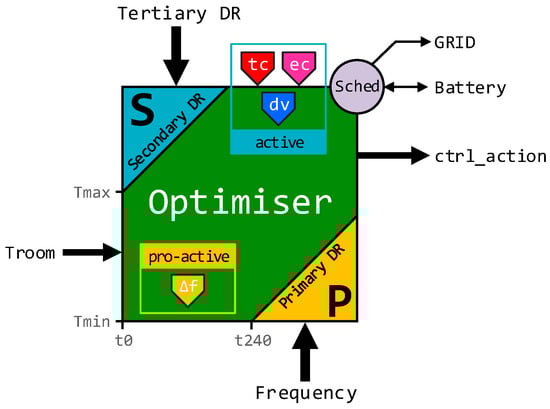
Figure 1.
A demand response (DR) framework block diagram.
The inclusion of building occupant feedback is crucial. Recent research has illustrated that engineers tend to assume occupants will not feel small changes in temperature [44]. This oversight can cause a performance gap between the expected and actual results from technologies intended to reduce or shift energy consumption in buildings. The inclusion of occupant feedback ensures that this issue will be avoided in the case of the solution presented in this paper.
This work provides a reference basis for further DR applications in decentralized community-based environments. It is particularly relevant to microgrids that are isolated from the grid as it offers potential for reducing the amount of energy storage required to balance the power fluctuation on those isolated microgrids. Current research has shown that even in the case of a single consumer, a microgrid option could be more economical than network renovation (e.g., provision of underground cabling) to increase the grid reliability [54]. Therefore, the ability to reduce the costs further by utilizing the approach described in this paper could offer real potential for the development of islanded and semi-islanded microgrids in many contexts.
2.2. General Description
The proposed decentralized, informatics, optimization, and control simulation model has been developed to optimize space heating, schedule utility of energy storage assets, and provide pro-active/active control for primary and secondary DR services. Two groups define the simulation model data that aims to replicate the trajectory of the physical systems under consideration so that system configuration parameters can be differentiated from local preferences. Ultimately, the simulation model is designed to assess our understanding of the optimizer and control components in the context of decentralized energy management. The applicability of the optimizer and control component is further demonstrated in hardware-in-the-loop simulation.
The following outline is provided as an overview of the proposed optimization and control strategy. The approach is based on the idea that when the demand for electricity on the distribution network is high, then the system attempts to reduce the local rate of energy consumption by reducing the space heating temperature setpoint. Similarly, during periods of low electricity demand the constraints that govern the temperature setpoint are relaxed, which, in turn, allows, not mandates, an increase in energy consumption by increasing the space heating temperature setpoint.
When we add a measured response from occupants that describes their collective relative thermal comfort, the perception is the rate of energy consumption shifts towards being self-regulatory. For example, if the demand for electricity increases, the system attempts to reduce the local energy consumption at a rate that is inversely proportional to the predicted demand. If space remains void of occupants, this approach is satisfactory and local settings ensure a minimum space temperature is maintained. However, during periods of occupancy, individuals become eligible participants in the optimization algorithm. Subsequently, when individuals report they are feeling cold, and their collective measured response satisfies a set threshold, then the resultant action is to issue a command that counters the instruction to reduce the space temperature further. Conversely, this self-regulatory behavior works equally well during periods of low demand. Consider now introducing a third data type. Incentivizing energy reduction through financial gain aims to reduce or shift energy consumption during periods of high demand [55].
Including information about the cost of energy into the mix introduces an interesting dynamic to the optimization and control strategy. Given a time of use tariff that increases at times when demand is known to peak, the net contribution to the optimizer is to automatically adjust the energy consumption when the cost of electricity exceeds a user-defined threshold. Furthermore, the system can be configured to automatically switch to an alternative power source if demand exceeds a set limit or during periods when the cost of energy makes utilizing an alternative power source more attractive, e.g., energy storage assets.
The immediate outcome attributed to the interaction between the three data types becomes even more attractive if their behaviors can be predicted over a finite time horizon. The opportunity to participate in tertiary DR services by making ready the system in response to a network operator DR instruction becomes feasible. The proposed control algorithm alters the demand profile trajectory such that it adds bias to the tri-data mix in a way that promotes a rise in space temperature. The net effect is to provide optimal space pre-heating in advance of commencing the scheduled DR event. Furthermore, a switching mechanism denies use of a local energy storage asset for a period leading up to the DR event. Instead, resources ensure the energy storage asset is set to recharge. Thus, when the DR event period commences, the system power source automatically switches to the energy storage asset. Previous interventions ensure the energy storage asset capacity is sufficiently charged to enable it to remain the primary source for the duration of the event or until the asset can no longer meet the power demand for continued operation. In this instance, the grid becomes the systems primary power source, and recharging of the energy storage asset is initiated.
The remainder of the section describes the development of individual systems that contribute to the optimization and control framework. Real-time computer simulations that aim to model the behavior of physical systems and the mathematical model of the proposed optimization and control algorithms are performed using the MATLAB/Simulink® environment. Level-2 MATLAB System functions have been used extensively during the design and implementation, providing access to create custom blocks that support multiple input and output ports. Furthermore, this section describes how desktop simulations are reconfigured to validate the optimization and control algorithm using hardware-in-the-loop (HIL) simulation techniques.
The desktop simulation model is shown in Figure 2. In addition to the optimization and control block, the model is composed of a catalogue of supporting subsystems: energy, building, scheduler, date-time (dt), and demand event signal (des).
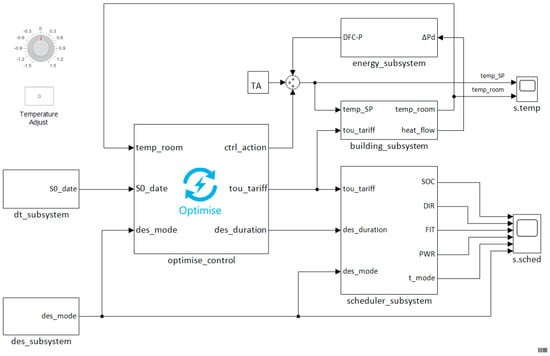
Figure 2.
Simulink® model of energy optimization framework.
2.3. Technical Development
The simulation optimizer is constructed in a piecemeal fashion, progressing sequentially by solving problems centered on three data types: (1) thermal comfort, (2) electricity demand forecast, and (3) cost (tariff). In brief, during periods when the system is not responding to a tertiary DR activity, the active control process begins by calculating a predicted or actual value for each data type over a 4-h horizon window at 10 min intervals. Values are mapped onto a multi-dimensional array with a fixed number of rows (magnitude) and columns (time). A Dijkstra’s algorithm is then used to project the predicted values over the 4-h horizon window [56,57]. The contribution of each data type is then combined before -means clustering (see Reference [58,59]) is applied iteratively at each 10 min interval. The result yields a new path that follows the optimal temperature setpoint trajectory over the 4-h horizon window. For demand response applications, a model for building design can be successfully implemented using a simplified first-order plus dead time model [60]. Time constants of 10 to 30 min and dead-times between 0 to 5 min are typical [61]. Avoiding complex calculations is achieved by taking a pragmatic approach when determining model control actions. For example, the proposed optimizer has been configured to update the control action at a sample time 10 min.
Since the control objective is to minimize the deviations from a temperature setpoint, according to the system and user-defined rules, at discrete points in time, the optimal cost (shortest path) can be obtained by formulating a Dynamic Programming algorithm that proceeds backwards in time. The algorithm takes a sequence of -means centroid points, where each centroid represents a value that minimizes the total intra-cluster variance of all objects in each cluster. In simple terms, given a time horizon of 240 min, this equates to 24 stages, each separated by a 10-min interval. At each stage, there are 11 objects. A k-means algorithm is applied to find the centroid of the 11 objects, at each stage. These calculations result in a series of 24 centroids that contribute to formulating the shortest path.
The objects that belong to each cluster are derived from a series of functions that calculate occupants’ relative thermal comfort cost (), rate of energy consumption (demand forecast value) cost (), and energy cost (). Given this, a deterministic problem can be formulated in a finite space , which can be equivalently represented by a gridmap of fixed dimension; the problem starts from a source node , where , proceeds to , and progresses to the final node . An important characteristic of this activity is highlighted. In solving the shortest path problem, the source node and target node are revealed to the optimizer just before the first transition from begins. The trajectory of the shortest path from will follow a series of weighted edges that interconnect successive pairs of nodes, i.e., .
In the framework of the fundamental problem, minimizing the cost in a finite state space can be translated into mathematical terms:
where the cost of transition at is the centroid in a cluster of objects at stage from node to node .
For the problem to have a solution, each object centroid is constructed with -means++ algorithm. Here, after initially assigning a random object within a cluster as the first centroid, we compute the distance from each remaining object. Based on the square of these distances, a new centroid is defined. The process repeats until centroids are chosen. We formulate the objects in the following sections.
In addition, when the network operator issues an explicit DR instruction, the optimizer initiates a pre-programmed control strategy that changes the trajectory of subsequent control actions in a period leading up to and during the event window. However, it remains useful if the control actions continue to respond to facility or occupant needs during this mode of operation.
2.4. Optimize and Control Subsystem
The optimize and control subsystem (optimize_control) is a user-defined block written using the MATLAB S-Function application programming interface (API). The proposed optimization algorithm calculates the optimal space heating temperature according to the rate at which electricity is consumed (demand) and cost (tariff). Furthermore, the final temperature value is impacted by the occupants’ thermal responses to the combined thermal effect of the environment and physiological variables that influence the relative thermal comfort.
Figure 2 shows the Simulink® optimize and control block includes three input signals: (1) room temperature (temp_room), (2) current date and time (S0_date), and (3) a demand event signal that indicates the status of a tertiary DR service (des_mode). The block output signals provide: (1) a control signal (ctrl_action) that will alter the space heating temperature setpoint, (2) the current cost of energy usage (tou_tariff), and (3) an indication of the tertiary DR event duration (des_duration). The internal architecture of the optimize and control subsystem is shown in Figure 3.
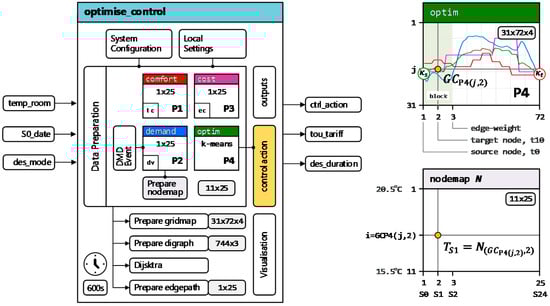
Figure 3.
Optimize and control internal block diagram.
The design presented in this article is configured to operate within a custom-built temperature range between and . Exception handling ensures temperature values measured outside this range are mapped to either or . Default system configuration parameters set the forecast horizon window to 4 h, a demand response temperature step () that instructs the control action to increase the space temperature by over the duration of the forecast horizon window, and the duration of a demand event to 40 min. Additional system parameters specific to thermal comfort, electricity demand forecasting and cost (tariff) are described in the corresponding subsections that follow.
2.4.1. Thermal Comfort
The energy demand of buildings is influenced by the presence and behavioral patterns of occupants [62]. The thermal comfort element impacts the temperature setpoint by analyzing the measured room temperature () and occupants’ feedback collated at a sample time of 10 min. Weekdays are divided into 7 time intervals , configured to mirror a typical teaching timetable, whereas a weekend day consists of only 1 time interval. Changing the weekend day interval pattern to replicate a weekday is straightforward. By considering occupant presence is inhomogeneous, for each we choose an algorithm for the simulation of occupants to be used as an input for current occupant level, . In practice, not all individuals will report their relative thermal comfort; therefore, the model automatically creates several feedback reports , where . An individual’s response is measured using a unipolar Likert scale [63,64]. The question has a five-scale response: too warm, warm, okay, cold, too cold; this is scored mathematically using a scale {−2, −1, 0, 1, 2}. In order to imitate perceived behavior patterns, for each time interval, the following model parameters are defined: , and response threshold . The thermal model weekday parameters are reported in Table 1.

Table 1.
Thermal model parameters.
For any given weekday time, the thermal comfort model output is calculated by the following expression:
with respect to:
s.t. constraints:
For weekend days, we assume ; hence, the model returns a value . The variation in represents a bias that is configured to reflect a change in outside temperature over a 24-h period.
It is noted that the seven-time intervals are bounded by a start and stop clock time such that , ; and terminating at . In practice, if a date and time are specified (e.g., S0_date = Fri, 05-February-2020 07:23:14), then the task to determine if the date-time element occurs on a weekday or weekend day is straightforward. Given a date-time S0_date, it is possible to formulate an algorithm that returns a array , where represents a thermal comfort value over a 4-h period at 10 min. It should be noted that because the optimizer is designed to take into consideration occupants’ feedback in real-time at a sample time of 10 min . However, if during the 4-h horizon window the system identifies a time interval where , i.e., there are no planned occupants, the model starts a pre-programmed sequence that sets the thermal comfort on a downward trajectory reducing at a rate of per 10 min interval until a minimum temperature threshold value .is reached. We have by the definition of the nodemap completed the data preparation of thermal comfort shown in Figure 3. It must be remembered that the thermal comfort model is prepared for operation within the simulated environment only. In practice, the implementation proposes occupants’ report thermal comfort to the system using a smartphone app. This concept is elaborated further in Section 3.
2.4.2. Electricity Demand Forecasting
A data-driven methodology for modeling electricity demand forecasting is proposed [65]. The implication of this novel semi-autonomous simplified lumped model has the potential to offer decentralized electricity network operators’ knowledge of the more extensive aggregated rate of future energy consumption. Thus, enabling decentralized energy management systems to proactively reduce load demand on small island electricity grids or distributed grid-edge systems as part of an evolving DR service. In this paper, we integrate the electricity demand forecasting model as part of the optimize and control framework. Initially, analysis of a chronological sequence of 245,424 discrete observations reveals the composition of the one-dimensional time series is characterized by three seasonal patterns: weekday, weekend day and month. These findings motivate an effort to reduce the dimensionality using piecewise aggregated approximation (PAA). Subsequently, calculating a cubic polynomial that interpolates points of interest yields a multi-dimensional array, which in turn helps restore the shape of the original demand forecast profile. The polynomial coefficient structure for weekday and weekend day are listed in the array page 1 and 2, respectively. Given both weekday and weekend day demand profiles recur every 24 h, it turns out using Equation (6) a normalized demand forecast value can be tagged to a specific time in any 24-h period.
where and correspond to the minimum and maximum data points of each PAA 2h segment, respectively, and the cubic polynomial coefficient parameters are , , , and . Moreover, we will show how the demand forecasting model can be used to compute a credible demand forecast value for any given date and time.
There are 12 equidistant segments, which equates to 13 periods () bounded by minimum and maximum points and , i.e., where the number of periods . In the first period, , after that ; and terminating at . If we adopt the convention that makes 13-time intervals bounded by a start and stop clock time then , after that ; and terminating at . Thus, it can be seen, given a date-time S0_date it is possible to formulate an algorithm that returns a array where represents a normalized demand forecast value over a 4-h period at min starting from the specified date-time. This approach works equally well for both weekdays and weekend days.
The normalized demand forecast value is defined as:
where , , , , noting that a nodemap is a two-dimensional array.
2.4.3. Cost (Tariff) Model
A key consideration when taking part in a predefined energy reduction strategy must empower customers to use energy in the lowest price period accessible, at the same time as offering participation in DR initiatives. The cost (tariff) model is configured to integrate a typical static time of use (TOU) tariff [66]. As shown in Figure 4, these tariffs charge cheaper rates when demand is low but increases for electricity consumption at peak times.
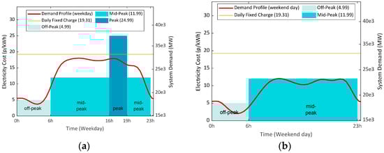
Figure 4.
Model static time of use (TOU) tariff: (a) Weekday; (b) Weekend day.
Given a date-time S0_date, the cost (tariff) model returns a array where represents a normalized cost (tariff) value over a 4-h period at min starting from the specific date-time.
The normalized cost (tariff) value is defined:
where is the cost (tariff) at min, , , , and . The scaling factors are set by design to position values in the subsequent optimize stage such that a change in price to either off-peak or peak has maximum influence during the optimization outcome. Furthermore, it will be shown impacts the operation of system assets managed by the scheduler subsystem.
2.4.4. Optimization
The optimization cycle (Figure 3) starts on receipt of the input signal S0_date. Subsequent cycles commence at a block sample time of 10 min (600 s). Previously, data preparation for occupants’ thermal comfort, electricity demand forecast, and cost (tariff) each returned a array where represents a normalised data type ( and ) value over a 4-h period at min intervals starting from a specific date-time (S0_date). Before each data type array can be processed, it must be homogenized in a way that makes it accessible to the optimizer. The data is transformed into a two-dimensional nodemap such that . Accordingly represents a temperature and defines 25 stages ) each separated by a 10 min time interval for the duration of the 4-h forecast horizon window, e.g., and is linked to the 10 min time interval . The nodemap is then transformed to a gridmap by the following function:
where:
s.t. constraints:
when constraint (13) is not satisfied .
The temperature from , where s.t. ; however, if , then ; furthermore, if , then . Based on this information, this equates to 31 permissible temperature changes between and . If we continue to record the change in temperature from using blocks of three columns for each cycle, then it is clear a gridmap of size is created. We refer to the three columns in each block as the source node , target node , and edge-weight , respectively.
The Dijkstra’s algorithm computes the shortest path between a specified temperature point given at and . This deterministic problem follows the principle of optimality which suggests if the path taken transits from one legitimate node to the next minimizes the cost-to-go from to , then the transition between the collective nodes must be optimal [67]. For the Dijkstra’s algorithm to solve the shortest path, the gridmap is first subjected to a series of simple transformations. The first instruction reshapes the gridmap into a matrix referred to as the edgelist. Here, following the same convention to identify columns in the gridmap, the edgelist provides a listed description of all source nodes , legitimate target nodes and their respective connecting edge-weights , i.e., its associated cost. A second instruction creates a digraph object that generates an Edges variable ( table) based on the number of source and target nodes extracted from the edgelist, and a Nodes variable ( table). The 275 value represents the total number of nodes () in the fixed nodemap. Finally, an equivalent sparse adjacency matrix representation of the digraph, which includes the edge-weights, is created. Since the graph object we have constructed is a directed graph, the sparse adjacency matrix is not symmetric. However, we can overcome this by converting the sparse adjacency matrix to a full storage matrix. In this instance, the conversion generates a full storage matrix.
The data type shape is now in a format required by the Dijkstra’s algorithm. Executing the Dijkstra’s algorithm will compute the optimal cost which is equivalent to the summation of all edge weights on the shortest path from to between time and .
This process is repeated for each data type. At the end of each transformation the results are assigned to a specific page of a multi-dimensional array where page 1 (P1) is reserved for data type comfort, page 2 (P2) demand, and page 3 (P3) cost (tariff). The fourth page (P4) is reserved for the final stage in the optimization process, which combines the contributions assigned to P1 to P3. Here, every third column in the P4 gridmap is allocated a grid centroid value , where and , and assigned to row index that is equivalent to the -means cluster centroid index that partitions the observations in the corresponding column on P1 to P3. Note, for each data type ; see Equation (1). The remaining values in each column are incremented by one until the row index has reached its boundary limit, i.e., or . When the Dijkstra’s algorithm subsequently computes the shortest path between the source node and target node where , the results yield the optimal path that transits from . The control action . Simply stated, the control action is a fixed temperature value that is linked to the nodemap at row index , where , where . The relationship between the gridmap and nodemap is highlighted in Figure 3. The pseudocode describing the operating principle of the optimize and control algorithm is listed in Appendix A.
2.5. Demand Event Signal Subsystem
The demand event signal subsystem (des_subsystem) simulates actions in response to a network operator instigated instruction. These signals are sent to individual customers enrolled in a campaign designed to deliver aggregated tertiary DR. The Simulink® model itself is trivial (Figure 5); however, the subsequent sequence of events requires further explanation. Firstly, the objective shifts to making the system ready for a DR event; this includes setting the control action to increase the room temperature in a measured approach by a pre-set value within the 4-h horizon window. Secondly, there is the objective to ensure the battery energy storage system (BESS) is available with enough charge at the start of the DR event.
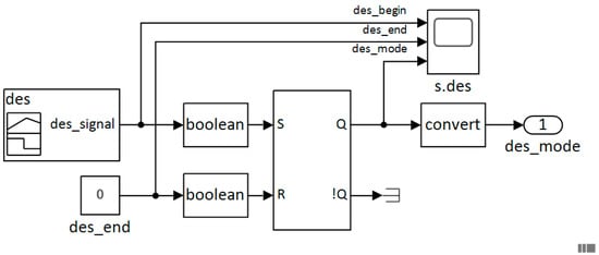
Figure 5.
Simulink® model of demand event signal subsystem.
The period of pre-heating is regulated by altering the demand forecast profile. By default, . Therefore, the normalized demand forecast value is recast to , where , , where s.t. . This new trajectory increases the last recorded room temperature by at a rate of every 50 min. At the beginning of each subsequent optimization cycle, the trajectory leading up to the DR event is maintained, i.e., it advances closer to the plus temperature at each iteration and towards the DR projected start time. However, before reverts to , the trajectory is modified further, this time by reducing the temperature setpoint less than the temperature recorded immediately before the start of the tertiary DR event. The system reinstates immediately after the DR event terminates.
The des_mode signal triggers the scheduler subsystem to start charging the BESS. The energy storage asset will continue to charge until the start of the DR event. The battery will then start to work from this time, reducing the stored charge of the battery while it continues to provide primary power to the heating system. The heating system will continue to be supplied from the battery until a state of charge (SOC) minimum threshold has been reached. The scheduler switches primary power to the grid and the battery to charge.
2.6. Energy Subsystem
Decentralized DR frequency regulation, when used in building stock, can regulate short-term frequency excursions in demanded electrical energy [68]. The contribution of a decentralized frequency regulator has been analyzed [68]. Results presented suggest that small excursions in measured temperature from a TCL setpoint value will not compromise indoor comfort temperatures but can contribute to the restoration of frequency equilibrium during network stress events. In this paper, we integrate the implied linear power system and frequency regulator as part of the optimize and control framework. The model (energy_subsystem) shown in Figure 6 replicates a power system rating of 300 MVA. Initial conditions assume the balance in supply and demand is at equilibrium, measured frequency is 50 Hz and the steady-state frequency error is zero. The energy subsystem model parameters are reported in Table 2.
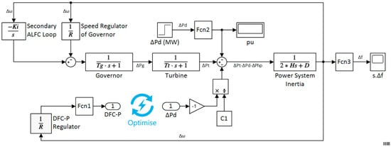
Figure 6.
Simulink® model of energy subsystem.
Table 2.
Energy subsystem parameters.
2.7. Building Subsystem
The building subsystem model (building_subsystem) (Figure 7) is a simplified thermostatically controlled (on/off) space heating system with feedback loops which typically maintains the air temperature at a set level. The model emulates building thermodynamics (building), calculating variations in temperature based on heat flow, , and heat losses, .
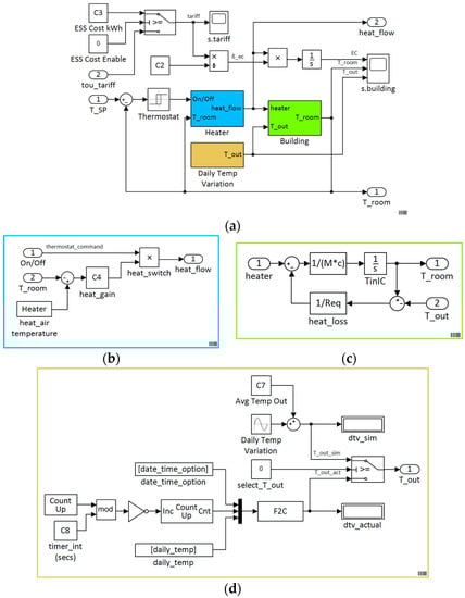
Figure 7.
Simulink® model: (a) Building subsystem; (b) heater; (c) building; (d) daily temperature variation.
A series of embedded lookup tables representative of seasonal variation are used to model outside air temperature over a 24-h period at a sample rate of 30 min [69]. In practice, the local outdoor temperature is measured using sensors and input into the system. Energy cost [p/kWh]) is calculated as a function of time and heat flow and is expressed in following equation:
where denotes air mass flow rate through the heater; specific heat at constant air pressure, and [p/kWh] is the energy price at time . The building subsystem model parameters are reported in Table 3.
Table 3.
Building subsystem parameters.
2.8. Scheduler Subsystem
The scheduler subsystem primary job is to monitor several signals and direct the operation of an automatic transfer switch between a grid and an alternative backup source of power. To ensure the appropriate power source is selected, the scheduler requires knowledge of the current cost (tariff) of electrical energy, whether a tertiary DR event is in progress including information of the event duration and BESS state of charge. The Simulink® model of the scheduler subsystem is shown in Figure 8 and includes three input signals and six output signals. The output signals are provided for visual indication of various signal status. A simplified BESS element (ess_subsystem) simulates a battery SOC using a first-order transfer function. Locally defined parameters SOC_hi and SOC_lo set maximum and minimum state of charge values (expressed as a percentage), which determine when the BESS is declared available for use. In this context, initial values are defined in Section 3. The model also includes a self-discharge rate (SDR) which reduces the stored charge of the battery naturally over time.
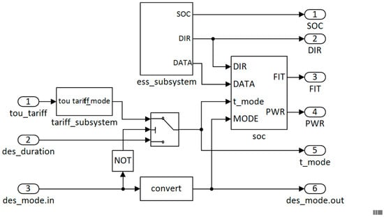
Figure 8.
Simulink® model of scheduler subsystem.
The BESS availability function is represented by Equation (17), where is a low-level SOC threshold (locally defined parameter).
Control rules that determine when the primary power source is set to grid or BESS is illustrated in Figure A1 (Appendix B). The decision variable t_mode is the cost (tariff) threshold and automatically switches the power source to BESS when the cost (tariff) is high s.t. Equation (17). Furthermore, when signal des_mode =1 (0 = normal, 1 = tertiary DR event), t_mode = 0, thus preventing a control action that switches the power source to BESS during the period leading up to the start of the DR event (nominally 4 h). Signal CDir (change direction) reports if the battery is in charge or discharge (0 = discharge, 1 = charge); PWR denotes primary power source (0 = grid, 1 = BESS); SOC_EC denotes cost (tariff) in use, (0 = TOU, 1 = BESS).
2.9. Date-Time Subsystem
For completeness, the Simulink® model of the date-time subsystem (dt_subsystem) is shown (Figure 9). Its primary function is to provide a date-time element at a sample time of 10 min. The model has been configured to run in real-time during experimental evaluation. By default, dt is set to the current date and time, using format dd-mmm-yyyy hh:mm:ss, with the option to set to any data time during model analysis. The date-time model parameters are reported in Table 4.
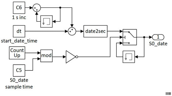
Figure 9.
Simulink® model of date-time subsystem.
Table 4.
Date time subsystem parameters.
3. Computational Study
In this section, we report the findings from a computational study (desktop simulation). By design, the computational study validates the functionality of critical services. In contrast, the experimental evaluation (Section 4) is explicitly directed on proving the interaction of proposed data types within the optimization subsystem. A simulated tertiary DR event is considered in both scenarios.
The interaction between decision variables and control actions of individual subsystems is complex. Accordingly, the computational study validates the functionality of the following vital services:
- Thermal comfort model
- Electrical demand forecasting model
- Cost (tariff) model
- Optimizer
- Tertiary DR activity
- Pro-active frequency control
To begin, we evaluate the data input models. Individual charts created using nodemap data, and corresponding gridmap data validate the optimization and control behavior. In the second study, the results obtained from a simulated tertiary DR event are discussed. Finally, we monitor the system behavior during an imbalance between supply and demand. Here, the pro-active frequency control reacts to a simulated load disturbance causing a frequency excursion from the nominal 50 Hz steady-state. The model is initialized using the values reported in Table 5.
Table 5.
Computational model initialization parameters.
Occupant thermal comfort feedback is shown in Figure 10a. At 16:40, the model reports the aggregated occupant thermal comfort is “too warm”. This consensus triggers the optimization algorithm to set the comfort level gridmap trajectory on a path that reduces the measured room temperature by , i.e., , where . In addition, according to local settings, the timetable sets the number of occupants in a space to zero at 19:00. A ‘no occupancy’ status has clearly defined adaptive triggers. Firstly, the comfort signal values (occupants, response, and comfort) are held at a constant zero, while the number of occupants present in a space is zero. Secondly, at 19:00, the optimizer begins to alter the comfort level gridmap trajectory by reducing the temperature to a minimum temperature threshold .(local setting) at a rate of every 10 min. This behavior is confirmed in the optimizer gridmap visualization and subsequent optimizer nodemap shown in Figure 11.
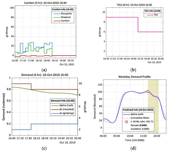
Figure 10.
Gridmap visualization of data type function response at 10-Oct-2019 16:00 over a 4-h horizon window: (a) Occupant thermal comfort feedback response; (b) electricity demand forecast: weekday 24 h; (c) cost (tariff); (d) electricity demand forecast.
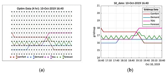
Figure 11.
Optimization response showing individual data types and forecast response: (a) gridmap visualization; (b) gridmap projected onto nodemap.
The price in the three-tier TOU tariff is translated visually in Figure 10b. Initially, from 16:00 to 19:00 the TOU signal value is set to 9, which represents cost 24.99 p/kWh (peak), reducing to 6 (11.99 p/kWh mid-peak price) at 19:00. The energy cost nodemap data () transformation to the optimizer gridmap is shown in Figure 11. During peak periods, when the cost of energy is highest, the gridmap interpretation is to influence the control variable by reducing the temperature setpoint, which in turn reduces the cost of energy. Similarly, at 19:00 (mid-peak), the gridmap tou signal is set at mid-scale (nominally ). The electricity demand forecast is shown in Figure 10c. To help interpret the demand signals shown, Figure 10d illustrates the calculated weekday demand profile over a 24-h period. The red circle marks the start of the 4-h horizon window (shaded area). The dv (gridmap) signal is reconstructed within the optimization algorithm. The results are consistent with the modified layout of corresponding digraph object node coordinates, which describes the relationship between directional edges and connecting nodes shown in Figure 11a. The optimal temperature path is calculated at a sample rate of 10 min. Figure 11b highlights the optimal temperature value over a 4-h horizon window commencing 16:40. The control action for the continuing 10 min cycle shown is the temperature value specified at 16:50, that is . This accords with our earlier occupant thermal comfort feedback report, which registered a consensus to reduce the room temperature by .
On receipt of a DR event notice (16:40) the normalized demand forecast value is recast to . The modified demand profile trajectory is defined by the Dijkstra’s shortest path algorithm , where . As can be observed in Figure 12, the change in demand profile at 16:50 increases from () to (). A sample rate of 600 s accounts for the slight delay from the start of the DR preparatory window to the change in demand profile trajectory. Although the supposed outcome is to promote an increase in temperature equivalent to leading up to the start of the DR event, the projected value is offset by the continued influence of the thermal comfort () and energy cost () (tou) decision variables. Consequently, in this instance, the optimization algorithm sets the 4-h ahead optimal temperature value slightly less than the anticipated . The layout of individual digraph objects and their corresponding nodemap representation, shown in Figure 11 and Figure 12, respectively, serve to provide a snapshot of the optimizer outputs over a 4-h horizon window at any given time. The benefit of the optimizer is now translated into Figure 13, which plots several decision variables and control actions over a 24-h period. Between Figure 13a,b, we observe the impact of demand and tariff data on the temperature setpoint (TS1). Furthermore, the outside temperature (Tout) as no impact on the measured room temperature during this simulation.
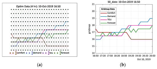
Figure 12.
Optimization response showing individual data types and forecast response on receipt of demand events signal, : (a) gridmap visualization; (b) gridmap projected onto nodemap.
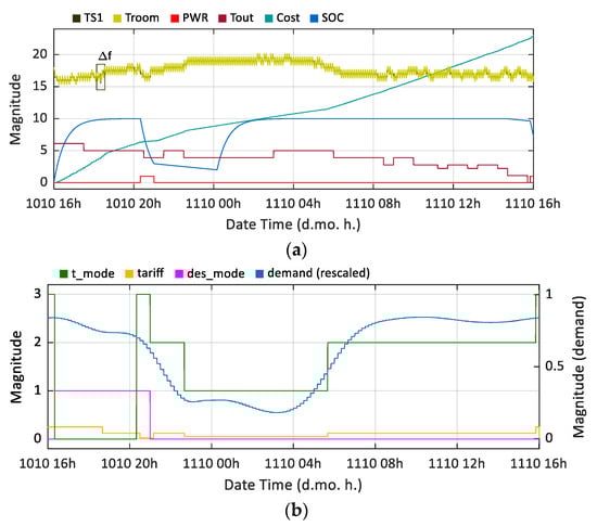
Figure 13.
Simulation study at 10-Oct-2019 16:00 for 24 h with DR event: (a) shows temperature setpoint (TS1), room temperature (Troom), primary power switch signal (PWR), outdoor temperature (Tout), cost (p/kWh) (Cost), and battery energy storage (BESS) state of charge (SOC) (%) (rescaled) (SOC) profiles; (b) shows tariff mode (t_mode), TOU tariff (tariff), demand event signal mode (des_mode), and demand (rescaled) (demand) profiles.
The start of the DR preparatory window is recorded at 16:40 and subsequently sets and holds des_mode = 1 for 4 h and 40 min (the time leading up to and including the DR event). The BESS is seen to start a charge period in readiness to the start of the DR event. A tariff mode signal (t_mode) automatically restricts the use of the BESS until the DR event starts. At 16:40, the power signal (PWR) switches the primary power source from the grid to BESS. If the cost of energy is peak tariff immediately after the DR event (t_mode = 3), then the BESS would continue as the primary power source. However, as can be observed, the BESS SOC signal (SOC) indicates the BESS starts a discharge phase at from the start of the DR event and continues, in this scenario, to the end of the DR event. At 20:20, the primary power source reverts to the grid, but the BESS remains available ().
The rate at which the energy source naturally discharges has been magnified to evaluate control actions when SDR exceeds low and high charge threshold values (local settings). In practice, SDR parameters should be set accordingly. The simulation results show the calculated electricity demand forecast profile (demand). Its impact on the optimization algorithm is clear when demand is high (06:00 to 22:00) the aggregated effect is to limit the temperature setpoint (reducing the demand for electricity on the distribution network). Conversely, when demand is low (22:00 to 06:00), the constraints that govern the temperature setpoint are relaxed. Here, the optimizer allows, not mandates, an increase in energy consumption by increasing the space heating temperature setpoint. This finding, while preliminary, suggests the proposed control strategy has the potential to deliberately lessen peaks in demand (electrical) and fill in the period of low demand.
At 18:20.36, the impact of a simulated load disturbance (Table 2) within the power subsystem is highlighted. The large and rapid decreasing frequency excursion shown in the box highlight, signifying an imbalance between supply and demand, is observed more clearly in Figure 14a. The proposed system immediate response is to lower the temperature setpoint (), reducing the on-site heat source energy consumption and thus providing a pro-active response to the stability of the electrical distribution network [68]. As can be observed in Figure 14b, and in the broader context in Figure 13a, these immediate interventions have minimal impact on measured room temperature (), hence minimizing occupant thermal discomfort.
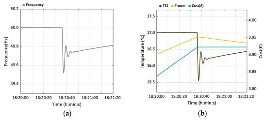
Figure 14.
Frequency response 10-Oct-2019: (a) impact on mains grid frequency due to simulated load disturbance; (b) proposed model response.
4. Experimental Evaluation
Testing cannot be expected to catch every error in the software, and system complexity makes it difficult to evaluate every branch. A traditional approach to software testing during earlier development and subsequent simulation testing provided a satisfactory level of acceptance. However, as the hardware-in-the-loop test environment is not entirely under the control of the tester, an element of nondeterminism is introduced in the test. Furthermore, because of observations documented during early simulation testing, new features are added to help eliminate transitions to deadlock states. These situations arise when a stalemate between two or more processes occurs, and the process is unable to proceed because each is waiting for the other to respond [70]. Therefore, it is considered helpful to outline an appropriate test and level of abstraction of the software and hardware devices for testing.
One of the significant objectives of testing is to assess the integration of the optimizer software code by connecting other software and hardware components. Therefore, a test environment was designed to evaluate and report as accurately as possible on the proposed optimization algorithm interaction with real-world data. An image of prototype equipment, including an industrial controller and sensor equipment, is shown in Figure 15a.
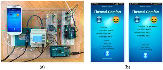
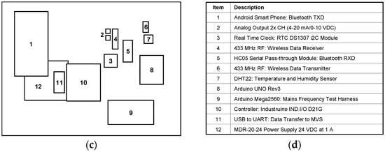
Figure 15.
Hardware-in-the-loop test environment: (a) Arduino equipment; (b) Android smartphone demonstrator app example screen images; (c) Arduino equipment block identification map; (d) Arduino equipment legend.
The test environment composed of the following main components: (1) a revised Simulink® model designed to send/receive serial data, (2) electronic fan speed controller (EFSC) to regulate the heat transfer through flow, (3) a 240 VAC 3 kW box fan portable heater, (4) an Industruino IND.I/O 32u4 Arduino-compatible industrial controller, which includes 2 CH 0 to 10 VDC/4-20 mA 12bit output, and (5) Arduino-compatible remote sensors and communication equipment, including Android smartphone pre-loaded with an app, developed using MIT App Inventor 2 version nb183c. In addition to streaming data into the software environment, the industrial controller on-board liquid crystal display (LCD) panel was codified to visualize the data from remote sensors and user thermal preferences (registered using the smartphone app). These feedback indicators were supplemented by a series of light emitting diodes (LEDs) reporting the status of several decision-making variables.
Dedicated values for energy demand forecasting and price indicators are embedded in the computer model. However, occupant thermal comfort feedback data is input into the system in real-time using Bluetooth technology. This experiment utilizes the thermal comfort feedback data reported by a single occupant. A technology update to manage multiple users is a relatively straightforward task. Images of the App demonstrator designed to capture occupants thermal comfort report is shown in Figure 15b. Remote sensors monitor room temperature data, which is communicated to the optimizer in real-time using low power device 433 MHz (LPD433) equipment. A block diagram of the general arrangement is shown in Figure 16. The positioning of the optimizer indicates this configuration has the potential to participate in similar energy management schemes with minimal impact on existing infrastructure.
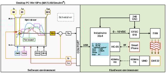
Figure 16.
Block diagram of experimental evaluation setup.
This paper reports the results of an experimental test carried out in real-time. The test started on Monday, 6-April-2020, 16:00. At 16:40, the start of a DR preparatory event triggers a pre-set sequence of control actions designed to prepare the heating services in advance of the 40 min DR event, which started at 20:40. The test was run for 5.5 h, finishing 10 min after the DR event. Comparison of the findings shown in Figure 17 with those of earlier computation studies confirms the operation of the optimization algorithm is consistent with our mathematical arguments, which posits that the interaction between declared data types can influence an environment space heating. Increasing the temperature setpoint successively by at 10-min intervals during the DR preparatory stage increased the space temperature by from the start of the DR preparatory window. Figure 18a confirms a temperature value of was recorded at approximately 19:10. It can be observed the temperature then decreased to at 20:40, which is the start time of DR event. This behavior may be explained by the fact that the thermal comfort profile (dark red color) reduced to an equivalent of () at 19:00, which is consistent with an expected zero occupancy at the same time.
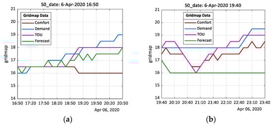
Figure 17.
Visual representations of gridmap data showing 4-h horizon window of predicted values of each data type and optimized temperature profile: (a) on receipt of a simulated DR event signal at 16:50; (b) during the 40 min DR event (20:40 to 21:20).
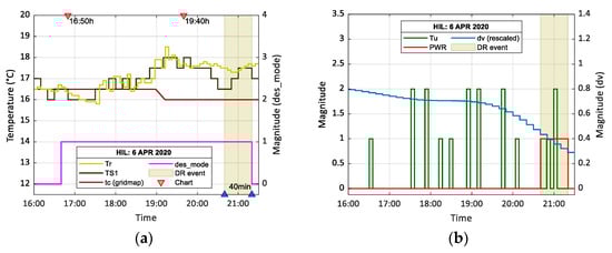
Figure 18.
Experimental evaluation recorded results at 6-April-2020 16:00 for 5.5 h with DR event: (a) room temperature (Tr), temperature setpoint (TS1), thermal comfort gridmap data (tc), demand event signal mode (des_mode), and DR event; (b) control action signal (Tu), primary power switch signal (PWR), demand (rescaled) (dv), and DR event.
Furthermore, as can be observed in Figure 18b, the control action signal utilized in the earlier computational study has been modified to regulate the physical heat transfer through flow. Here, the control action signal (Tu), which operates a 0 to 10 VDC EFSC, is proportional to the difference between the calculated optimal temperature setpoint (TS1) and the measured temperature (Tr), i.e., , where . The power switch signal (PWR) shows the virtual energy storage system is activated at 20:40 and continues to operate as the heating system primary energy source for the duration of the DR event (shaded area).
Overall, these results are very encouraging. The experimental evaluation raises the possibility that the proposed optimization algorithm may support small communities in a decentralized environment with limited access to communication networks. Comparison of the findings with other studies confirms the novelty of the proposed framework for energy management. It is encouraging elements of this research are consistent with results found in previous work. Eriksson et al. [71] developed a normalized weighted constrained multi-objective meta-heuristic optimization algorithm to consider technical, economic, socio-political, and environmental objectives. The results emphasized the application of a modified Particle Swarm Optimization (PSO) algorithm to optimize a renewable energy system of any configuration. The implementation of the Dijkstra’s algorithm (used in this study) is more prevalent in other applications (e.g., see Reference [72,73,74]).
Nevertheless, the simplicity Dijkstra’s algorithm makes it a versatile heuristic algorithm. The shortest path optimization algorithm was designed to compute an optimal water heating plan based on specific optimality criteria and inputs [75]. The significant feature reported of the proposed algorithm was its low computational complexity, which opens the possibility to deploy directly on low-cost embedded controllers. In a further study, a strong relationship between optimization and space heating has been reported [76]. Here, a neural network algorithm was used to build a predictive model for the optimization of a HVAC is combined with a strength multi-objective PSO algorithm. Although results show satisfactory solutions at hourly time intervals for users with different preferences, demand response mechanisms have not been considered. However, leveraging upon the concepts of Industry 4.0, Short et al. [77] demonstrated the potential to dispatch HVAC units in the presence of tertiary DR program in a distributed optimization problem could deliver satisfactory performances. Finally, a more inclusive study proposed an optimization model which takes total operational cost and energy efficiencies as objective functions [78]. Here, a thermal load is adjusted in the knowledge that a managed change in temperature value has no significant impact on user comfort. An integrated demand response mechanism is also considered. Although the results provide a new perspective for integrated energy management and demand side load management, there is no further exploitation in real-time user engagement or perspectives on decentralization.
5. Conclusions
A real-time DR strategy in a decentralized grid has been formulated with both spatial and temporal constraints. A generic framework established regulatory control of space heating through mechanisms that automatically respond to changes in grid frequency and in response to explicit tertiary DR event signals. Design considerations set decision variables and control actions to illustrate the effectiveness of the novel multi-objective cost function, which is based on a weight-based routing algorithm. A series of embedded lookup tables based on historical operational data calculate an aggregated rate of electricity consumption over a rolling 4-h horizon window. As the techniques for enabling and controlling DR events emerged, extensive simulation studies demonstrated power consumption could be easily shifted without causing any significant short-term impact on space temperatures. Increasing growth of renewable energy resources could reduce system inertia, which means networks are more vulnerable to energy security. The approach offered may benefit rural decentralized community power systems, including geographical islands, seeking to optimize heating services through optimization and collaborative energy management. This operation was validated using experimental testing, which included a response to simulated tertiary DR event signals. The obtained results show an effectiveness of the decentralized, informatic optimization, and control framework for evolving DR services. The energy transition offers small communities’ opportunities to meet decarbonization targets. The gradual shift from centralized fossil fuel power networks to more low carbon decentralized sustainable smart energy systems is set to disrupt businesses, policymakers, and system analysts. As energy markets change to meet innovations, the reliance on a single energy source is slowly diminishing. Still, as technology advances and support for an emerging group of consumers that produce energy continues to gather momentum, system operators should embrace a changing market to remain relevant in the future.
The context within which DR operates is important as related initiatives need to support the objectives of DR itself. These are usually encased within a policy objective in response to concerns relating to the environment. Concerning supporting the achievement of such policy goals, organizations seeking to participate in the sector need a business model/strategy that will, in the longer-term support and sustain the success of such policy goals. Therefore, the business model is essential to the objective of the policy. Martin et al. [79] illustrated the dangers of applying the business model/strategy that does not support the overall objective of an organization. Here, the policy goal is the European targets related to energy efficiency and climate change by consumers reducing or shifting their electricity usage during periods of peak electricity demand in response to time-based tariffs or other forms of financial incentives. The success of such policy objectives, therefore, are dependent on several factors, including end-user participation. The opportunities for realizing DR, however, vary across Europe as they are dependent on the particular regulatory, market, and technical contexts in different European countries [80]. It is estimated that the distribution networks share of the overall network investment in energy networks will be 80% by 2050 [81]. Hence, the need for DR solutions to reduce peaks in energy demand is significant. Thus, in recent times, the emphasis is on developing novel solutions which can align the energy demand to the energy supply in real-time [82]. A decentralized approach will support creativity and tailor-made solutions [83,84]. The role of the end-user in successfully delivering the policy objective is essential, and their buying into new usage patterns is critical [85]. Therefore, a business model that encourages end-user participation becomes crucial. Hence, a business model that understands and appreciates the variables of regulatory, market and technical contexts in different European countries, enabling enhanced end-user engagement is required to support the achievement of the policy objectives.
Future research will extend the test and validation work, including the integration of scalable communities and other forms of energy storage and distributed renewable energy generators. In addition, a business case that scrutinizes how the proposed optimization and control framework can be mobilized will be investigated in future work.
Author Contributions
Conceptualization, S.W.; methodology, S.W.; software, S.W.; validation, S.W. and M.S.; formal analysis, S.W. and M.S.; investigation, S.W.; resources, S.W.; data curation, S.W.; writing—original draft preparation, S.W.; writing—review and editing, S.W., M.S., T.C. and M.S.-P.; visualization, S.W.; supervision, M.S. and T.C.; project administration, S.W.; funding acquisition, M.S. and T.C. All authors have read and agreed to the published version of the manuscript.
Funding
Elements of the work presented in this paper was carried out as part of the REACT project (01/01/2019-31/12/2022) which is co-funded by the EU’s Horizon 2020 Framework Programme for Research and Innovation under Grant Agreement No. 824395.
Acknowledgments
The first author wishes to acknowledge the financial support provided by Teesside University and the Doctoral Training Alliance (DTA) scheme in Energy.
Conflicts of Interest
The authors declare no conflict of interest. The funders had no role in the design of the study; in the collection, analysis, or interpretation of data; in the writing of the manuscript, or in the decision to publish the results.
Appendix A
| AlgorithmA1. Optimize and control algorithm |
| inputs: |
| temp_room = ▷ |
| S0_date ← now() |
| ▷ 0=normal, 1=event |
| outputs: |
| ctrl_action; tou_tariff; des_duration |
| initialise: |
| visual_mode; gridmap |
| horizon = 4 ▷ duration (h) |
| des_mode = 0 |
| () = |
| des_duration = ▷ duration (min) |
| = |
| = {tc, dv, ec, optim} |
| for every 10 min interval do |
| S0_date ← S0_date + 10 min |
| for each do |
| if = tc then |
| ▷ min temp threshold |
| prepare comfort values |
| else if = dv then |
| require: des_mode; des_duration; |
| prepare demand values |
| prepare node path |
| else if = ec then |
| prepare tou values |
| end if |
| get: |
| prepare gridmap |
| adjacency matrix ← digraph ← edgelist ← gridmap |
| optimize using dijkstra algorithm |
| identify edgepath from start to end node |
| if = optim then |
| prepare control action ▷ |
| end if |
| get: visual_mode |
| display: visualization ∈ {horizon, gridmap, bigpath, biggridmap} |
| end for |
| end for |
Appendix B

Figure A1.
Scheduler control logic flowchart.
References
- Alcott, B. Jevons’ paradox. Ecol. Econ. 2005, 54, 9–21. [Google Scholar] [CrossRef]
- Copiello, S. Building energy efficiency: A research branch made of paradoxes. Renew. Sustain. Energy Rev. 2017, 69, 1064–1076. [Google Scholar] [CrossRef]
- Harris, T.M.; Devkota, J.P.; Khanna, V.; Eranki, P.L.; Landis, A.E. Logistic growth curve modeling of US energy production and consumption. Renew. Sustain. Energy Rev. 2018, 96, 46–57. [Google Scholar] [CrossRef]
- Freire-González, J.; Puig-Ventosa, I. Energy efficiency policies and the Jevons paradox. Int. J. Energy Econ. Policy 2015, 5, 69–79. [Google Scholar]
- Vujanović, M.; Wang, Q.; Mohsen, M.; Duić, N.; Yan, J. Special issue of applied energy dedicated to SDEWES conferences 2018: Sustainable energy technologies and environmental impacts of energy systems. Appl. Energy 2019, 256. [Google Scholar] [CrossRef]
- Abdullah, M.A.; Agalgaonkar, A.P.; Muttaqi, K.M. Assessment of energy supply and continuity of service in distribution network with renewable distributed generation. Appl. Energy 2014, 113, 1015–1026. [Google Scholar] [CrossRef]
- Ratnam, K.S.; Palanisamy, K.; Yang, G. Future low-inertia power systems: Requirements, issues, and solutions—A review. Renew. Sustain. Energy Rev. 2020, 124, 109773. [Google Scholar] [CrossRef]
- Bayod-Rújula, A.A. Future development of the electricity systems with distributed generation. Energy 2009, 377–383. [Google Scholar] [CrossRef]
- Neelawela, U.D.; Selvanathan, E.A.; Wagner, L.D. Global measure of electricity security: A composite index approach. Energy Econ. 2019, 81, 433–453. [Google Scholar] [CrossRef]
- Kosai, S.; Unesaki, H. Short-term vs long-term reliance: Development of a novel approach for diversity of fuels for electricity in energy security. Appl. Energy 2020, 262, 114520. [Google Scholar] [CrossRef]
- IEA Statistics The World Bank. Available online: https://data.worldbank.org/indicator/EG.USE.COMM.FO.ZS (accessed on 14 April 2020).
- Price, J.; Zeyringer, M.; Konadu, D.; Sobral Mourão, Z.; Moore, A.; Sharp, E. Low carbon electricity systems for Great Britain in 2050: An energy-land-water perspective. Appl. Energy 2018, 228, 928–941. [Google Scholar] [CrossRef]
- Hope, A.; Roberts, T.; Walker, I. Consumer engagement in low-carbon home energy in the United Kingdom: Implications for future energy system decentralization. Energy Res. Soc. Sci. 2018, 44, 362–370. [Google Scholar] [CrossRef]
- Barrett, J.; Cooper, T.; Hammond, G.P.; Pidgeon, N. Industrial energy, materials and products: UK decarbonisation challenges and opportunities. Appl. Therm. Eng. 2018, 136, 643–656. [Google Scholar] [CrossRef]
- Foxon, T.; Hammond, G.; Pearson, P. Socio-technical transitions in UK electricity: Part 2 – technologies and sustainability. Proc. Inst. Civ. Eng. Energy 2020, 173, 123–136. [Google Scholar] [CrossRef]
- Johnstone, P.; Kivimaa, P. Multiple dimensions of disruption, energy transitions and industrial policy. Energy Res. Soc. Sci. 2018, 37, 260–265. [Google Scholar] [CrossRef]
- IRENA International Renewable Energy Agency. Renewable Power Generation Costs in 2018; IRENA: Abu, Dhabi, 2018. [Google Scholar]
- Imperial College London. Report prepared for Committee on Climate Change Final; Vivid Economics Limited: London, UK, 2019. [Google Scholar]
- Zheng, C.; Yuan, J.; Zhu, L.; Zhang, Y.; Shao, Q. From digital to sustainable: A scientometric review of smart city literature between 1990 and 2019. J. Clean. Prod. 2020, 258, 120689. [Google Scholar] [CrossRef]
- Sodiq, A.; Baloch, A.A.B.; Khan, S.A.; Sezer, N.; Mahmoud, S.; Jama, M.; Abdelaal, A. Towards modern sustainable cities: Review of sustainability principles and trends. J. Clean. Prod. 2019, 227, 972–1001. [Google Scholar] [CrossRef]
- Mosannenzadeh, F.; Bisello, A.; Vaccaro, R.; D’Alonzo, V.; Hunter, G.W.; Vettorato, D. Smart energy city development: A story told by urban planners. Cities 2017, 64, 54–65. [Google Scholar] [CrossRef]
- Wang, S.J.; Moriarty, P. Energy savings from Smart Cities: A critical analysis. Energy Procedia 2019, 158, 3271–3276. [Google Scholar] [CrossRef]
- Di Silvestre, M.L.; Favuzza, S.; Riva Sanseverino, E.; Zizzo, G. How Decarbonization, Digitalization and Decentralization are changing key power infrastructures. Renew. Sustain. Energy Rev. 2018, 93, 483–498. [Google Scholar] [CrossRef]
- Thellufsen, J.Z.; Lund, H.; Sorknæs, P.; Østergaard, P.A.; Chang, M.; Drysdale, D.; Nielsen, S.; Djørup, S.R.; Sperling, K. Smart energy cities in a 100% renewable energy context. Renew. Sustain. Energy Rev. 2020, 129, 109922. [Google Scholar] [CrossRef]
- Marinova, S.; Deetman, S.; van der Voet, E.; Daioglou, V. Global construction materials database and stock analysis of residential buildings between 1970–2050. J. Clean. Prod. 2020, 247, 119146. [Google Scholar] [CrossRef]
- Qiao, R.; Liu, T. Impact of building greening on building energy consumption: A quantitative computational approach. J. Clean. Prod. 2020, 246, 119020. [Google Scholar] [CrossRef]
- Paridari, K.; Nordström, L. Flexibility prediction, scheduling and control of aggregated TCLs. Electr. Power Syst. Res. 2020, 178, 106004. [Google Scholar] [CrossRef]
- Ibrahim, O.; Fardoun, F.; Younes, R.; Louahlia-Gualous, H. Review of water-heating systems: General selection approach based on energy and environmental aspects. Build. Environ. 2014, 72, 259–286. [Google Scholar] [CrossRef]
- Yang, L.; Yan, H.; Lam, J.C. Thermal comfort and building energy consumption implications—A review. Appl. Energy 2014, 115, 164–173. [Google Scholar] [CrossRef]
- Ascione, F.; Bianco, N.; Mauro, G.M.; Napolitano, D.F.; Vanoli, G.P. Weather-data-based control of space heating operation via multi-objective optimization: Application to Italian residential buildings. Appl. Therm. Eng. 2019, 163, 114384. [Google Scholar] [CrossRef]
- Lin, S.; Liu, D.; Hu, F.; Li, F.; Dong, W.; Li, D.; Fu, Y. Grouping control strategy for aggregated thermostatically controlled loads. Electr. Power Syst. Res. 2019, 171, 97–104. [Google Scholar] [CrossRef]
- Erdogan, S.; Yıldırım, S.; Yıldırım, D.C.; Gedikli, A. The effects of innovation on sectoral carbon emissions: Evidence from G20 countries. J. Environ. Manag. 2020, 267, 110637. [Google Scholar] [CrossRef]
- Kumar, D.; Mathur, H.D.; Bhanot, S.; Bansal, R.C. Modeling and frequency control of community micro-grids under stochastic solar and wind sources. Eng. Sci. Technol. Int. J. 2020. [Google Scholar] [CrossRef]
- Loisel, R.; Lemiale, L. Comparative energy scenarios: Solving the capacity sizing problem on the French Atlantic Island of Yeu. Renew. Sustain. Energy Rev. 2018, 88, 54–67. [Google Scholar] [CrossRef]
- Pfeifer, A.; Dobravec, V.; Pavlinek, L.; Krajačić, G.; Duić, N. Integration of renewable energy and demand response technologies in interconnected energy systems. Energy 2018, 161, 447–455. [Google Scholar] [CrossRef]
- Curto, D.; Favuzza, S.; Franzitta, V.; Musca, R.; Navarro Navia, M.A.; Zizzo, G. Evaluation of the optimal renewable electricity mix for Lampedusa island: The adoption of a technical and economical methodology. J. Clean. Prod. 2020, 263. [Google Scholar] [CrossRef]
- Cabrera, P.; Lund, H.; Carta, J.A. Smart renewable energy penetration strategies on islands: The case of Gran Canaria. Energy 2018, 162, 421–443. [Google Scholar] [CrossRef]
- Tindemans, S.; Strbac, G. Low-complexity control algorithm for decentralised demand response using thermostatic loads. In Proceedings of the Proceedings—2019 IEEE International Conference on Environment and Electrical Engineering and 2019 IEEE Industrial and Commercial Power Systems Europe (EEEIC/I and CPS Europe), Genova, Italy, 11–14 June 2019. [Google Scholar]
- Schellenberg, C.; Dimache, L.; Lohan, J. Grid-edge technology—Exploring the flexibility potential of a heat pump and thermal energy storage system. In Proceedings of the E3S Web of Conferences, Galway, Ireland, 13 August 2019. [Google Scholar]
- Shen, Y.; Li, Y.; Zhang, Q.; Shi, Q.; Li, F. State-shift priority based progressive load control of residential HVAC units for frequency regulation. Electr. Power Syst. Res. 2020, 182, 106194. [Google Scholar] [CrossRef]
- Croce, D.; Giuliano, F.; Bonomolo, M.; Leone, G.; Musca, R.; Tinnirello, I. A decentralized load control architecture for smart energy consumption in small islands. Sustain. Cities Soc. 2020, 53, 101902. [Google Scholar] [CrossRef]
- Esposito, C.; Tamburis, O.; Su, X.; Choi, C. Robust Decentralised Trust Management for the Internet of Things by Using Game Theory. Inf. Process. Manag. 2020, 57, 102308. [Google Scholar] [CrossRef]
- McLellan, B.; Florin, N.; Giurco, D.; Kishita, Y.; Itaoka, K.; Tezuka, T. Decentralised energy futures: The changing emissions reduction landscape. Procedia CIRP 2015, 29, 138–143. [Google Scholar] [CrossRef]
- Breukers, S.; Crosbie, T.; Van Summeren, L. Mind the gap when implementing technologies intended to reduce or shift energy consumption in blocks-of-buildings. Energy Environ. 2020, 31, 613–633. [Google Scholar] [CrossRef]
- Ala-Juusela, M.; Crosbie, T.; Hukkalainen, M. Defining and operationalising the concept of an energy positive neighbourhood. Energy Convers. Manag. 2016, 125, 133–140. [Google Scholar] [CrossRef]
- Crosbie, T.; Broderick, J.; Short, M.; Charlesworth, R.; Dawood, M. Demand response technology readiness levels for energy management in blocks of buildings. Buildings 2018, 8, 13. [Google Scholar] [CrossRef]
- Zapata Riveros, J.; Kubli, M.; Ulli-Beer, S. Prosumer communities as strategic allies for electric utilities: Exploring future decentralization trends in Switzerland. Energy Res. Soc. Sci. 2019, 57, 101219. [Google Scholar] [CrossRef]
- Brown, D.; Hall, S.; Davis, M.E. What is prosumerism for? Exploring the normative dimensions of decentralised energy transitions. Energy Res. Soc. Sci. 2020, 66. [Google Scholar] [CrossRef]
- Martínez Fernández, P.; Villalba Sanchís, I.; Yepes, V.; Insa Franco, R. A review of modelling and optimisation methods applied to railways energy consumption. J. Clean. Prod. 2019, 222, 153–162. [Google Scholar] [CrossRef]
- Borhanazad, H.; Mekhilef, S.; Gounder Ganapathy, V.; Modiri-Delshad, M.; Mirtaheri, A. Optimization of micro-grid system using MOPSO. Renew. Energy 2014, 71, 295–306. [Google Scholar] [CrossRef]
- Zizzo, G.; Beccali, M.; Bonomolo, M.; Di Pietra, B.; Ippolito, M.G.; La Cascia, D.; Leone, G.; Lo Brano, V.; Monteleone, F. A feasibility study of some DSM enabling solutions in small islands: The case of Lampedusa. Energy 2017, 140, 1030–1046. [Google Scholar] [CrossRef]
- Skjølsvold, T.M.; Ryghaug, M.; Throndsen, W. European island imaginaries: Examining the actors, innovations, and renewable energy transitions of 8 islands. Energy Res. Soc. Sci. 2020, 65, 101491. [Google Scholar] [CrossRef]
- Tindemans, S.H.; Trovato, V.; Strbac, G. Decentralized Control of Thermostatic Loads for Flexible Demand Response. IEEE Trans. Control Syst. Technol. 2015, 23, 1685–1700. [Google Scholar] [CrossRef]
- Uski, S.; Rinne, E.; Sarsama, J. Microgrid as a cost-effective alternative to rural network underground cabling for adequate reliability. Energies 2018, 11, 1978. [Google Scholar] [CrossRef]
- Bradley, P.; Coke, A.; Leach, M. Financial incentive approaches for reducing peak electricity demand, experience from pilot trials with a UK energy provider. Energy Policy 2016, 98, 108–120. [Google Scholar] [CrossRef]
- Dijkstra, E.W. A note on two problems in connection with graphs. Numer. Math. 1959, 1, 269–271. [Google Scholar] [CrossRef]
- Williams, S.; Short, M. Electricity Demand Forecasting in Decentralised Demand Side Response for Blocks of Building. In Proceedings of the International Conference on Energy and Sustainable Futures (ICESF), Nottingham, UK, 9–11 September 2019. [Google Scholar]
- Hartigan, J.A.; Wong, M.A. Algorithm AS 136: A K-Means Clustering Algorithm. Appl. Stat. 1979, 28, 100–108. [Google Scholar] [CrossRef]
- Cai, W.; Zhao, J.; Zhu, M. A real time methodology of cluster-system theory-based reliability estimation using k-means clustering. Reliab. Eng. Syst. Saf. 2020, 202. [Google Scholar] [CrossRef]
- Mathews, E.; Richards, P.; Lombard, C. A first-order thermal model for building design. Energy Build. 1994, 21, 133–145. [Google Scholar] [CrossRef]
- Bi, Q.; Cai, W.J.; Wang, Q.G.; Hang, C.C.; Lee, E.-L.; Sun, Y.; Liu, K.D.; Zhang, Y.; Zou, B. Advanced controller auto-tuning and its application in HVAC systems. Control Eng. Pract. 2000, 8, 633–644. [Google Scholar] [CrossRef]
- Happle, G.; Fonseca, J.A.; Schlueter, A. A review on occupant behavior in urban building energy models. Energy Build. 2018, 174, 276–292. [Google Scholar] [CrossRef]
- Likert, R. A Technique for the Measurement of Attitudes. Arch. Psychol. 1932, 22, 5–53. [Google Scholar]
- Joshi, A.; Kale, S.; Chandel, S.; Pal, D. Likert Scale: Explored and Explained. Br. J. Appl. Sci. Technol. 2015, 7, 396–403. [Google Scholar] [CrossRef]
- Williams, S.; Short, M. Electricity demand forecasting for decentralised energy management. Energy Built Environ. 2020, 1, 178–186. [Google Scholar] [CrossRef]
- Green Energy UK Green Energy UK. Available online: https://www.greenenergyuk.com/ (accessed on 31 March 2020).
- Bellman, R.E. The Theory of Dynamic Programming. Bull. Am. Math. Soc. 1954, 60, 503–515. [Google Scholar] [CrossRef]
- Williams, S.; Short, M.; Crosbie, T. On the use of thermal inertia in building stock to leverage decentralised demand side frequency regulation services. Appl. Therm. Eng. 2018, 133, 97–106. [Google Scholar] [CrossRef]
- Weather Underground Weather History & Data Archive. Available online: https://www.wunderground.com/history (accessed on 3 April 2020).
- Laneve, C. A lightweight deadlock analysis for programs with threads and reentrant locks. Sci. Comput. Program. 2019, 181, 64–81. [Google Scholar] [CrossRef]
- Eriksson, E.L.V.; Gray, E.M.A. Optimization of renewable hybrid energy systems—A multi-objective approach. Renew. Energy 2019, 133, 971–999. [Google Scholar] [CrossRef]
- Wang, H.; Mao, W.; Eriksson, L. A Three-Dimensional Dijkstra’s algorithm for multi-objective ship voyage optimization. Ocean Eng. 2019, 186, 106131. [Google Scholar] [CrossRef]
- Rosita, Y.D.; Rosyida, E.E.; Rudiyanto, M.A. Implementation of dijkstra algorithm and multi-criteria decision-making for optimal route distribution. Procedia Comput. Sci. 2019, 161, 378–385. [Google Scholar] [CrossRef]
- Shen, L.; Shao, H.; Wu, T.; Lam, W.H.K.; Zhu, E.C. An energy-efficient reliable path finding algorithm for stochastic road networks with electric vehicles. Transp. Res. Part C Emerg. Technol. 2019, 102, 450–473. [Google Scholar] [CrossRef]
- Kapsalis, V.; Safouri, G.; Hadellis, L. Cost/comfort-oriented optimization algorithm for operation scheduling of electric water heaters under dynamic pricing. J. Clean. Prod. 2018, 198, 1053–1065. [Google Scholar] [CrossRef]
- Kusiak, A.; Xu, G.; Tang, F. Optimization of an HVAC system with a strength multi-objective particle-swarm algorithm. Energy 2011, 36, 5935–5943. [Google Scholar] [CrossRef]
- Short, M.; Rodriguez, S.; Charlesworth, R.; Crosbie, T.; Dawood, N. Optimal dispatch of aggregated HVAC units for demand response: An industry 4.0 approach. Energies 2019, 12, 4320. [Google Scholar] [CrossRef]
- Wang, Y.; Ma, Y.; Song, F.; Ma, Y.; Qi, C.; Huang, F.; Xing, J.; Zhang, F. Economic and efficient multi-objective operation optimization of integrated energy system considering electro-thermal demand response. Energy 2020, 205. [Google Scholar] [CrossRef]
- Martin, M.; Pajouh, M.S. Rebalancing the balance: How the WTO’s HR policy impacts on its very objectives for welfare enhancement and development. J. Int. Trade Law Policy 2011, 10, 243–254. [Google Scholar] [CrossRef]
- Crosbie, T.; Short, M.; Dawood, M.; Charlesworth, R. Demand Response in Blocks of Buildings: Opportunities and Requirements. J. Entrep. Sustain. Issues 2017, 4, 271–281. [Google Scholar] [CrossRef]
- Eurelectric Union of the Electricity Industry. Power Distribution in Europe: Facts Figures; Eurelectric aisbl: Brussels, Belgium, 2013. [Google Scholar]
- Patteeuw, D.; Bruninx, K.; Arteconi, A.; Delarue, E.; D’haeseleer, W.; Helsen, L. Integrated modeling of active demand response with electric heating systems coupled to thermal energy storage systems. Appl. Energy 2015, 151, 306–319. [Google Scholar] [CrossRef]
- Pop, C.; Cioara, T.; Antal, M.; Anghel, I.; Salomie, I.; Bertoncini, M. Blockchain Based Decentralized Management of Demand Response Programs in Smart Energy Grids. Sensors 2018, 18, 162. [Google Scholar] [CrossRef]
- Mengelkamp, E.; Notheisen, B.; Beer, C.; Dauer, D.; Weinhardt, C. A blockchain-based smart grid: Towards sustainable local energy markets. Comput. Sci. – Res. Dev. 2018, 33, 207–214. [Google Scholar] [CrossRef]
- Radenković, M.; Bogdanović, Z.; Despotović-Zrakić, M.; Labus, A.; Lazarević, S. Assessing consumer readiness for participation in IoT-based demand response business models. Technol. Forecast. Soc. Chang. 2020, 150, 119715. [Google Scholar] [CrossRef]
© 2020 by the authors. Licensee MDPI, Basel, Switzerland. This article is an open access article distributed under the terms and conditions of the Creative Commons Attribution (CC BY) license (http://creativecommons.org/licenses/by/4.0/).