Use of Stirling Engine for Waste Heat Recovery


Abstract
1. Introduction
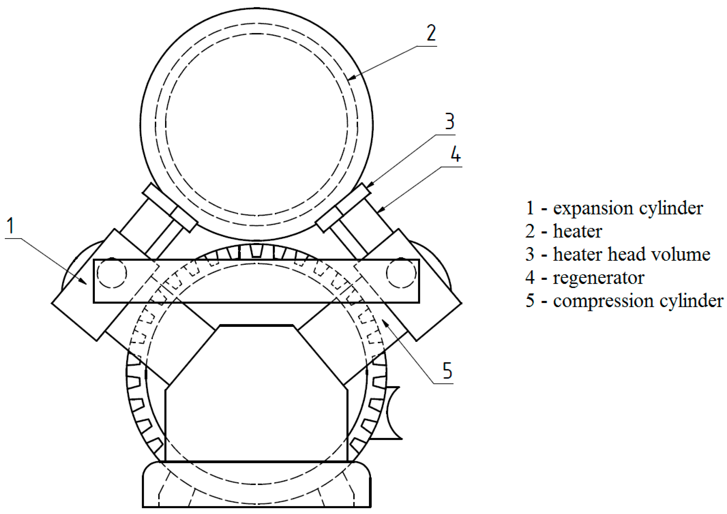
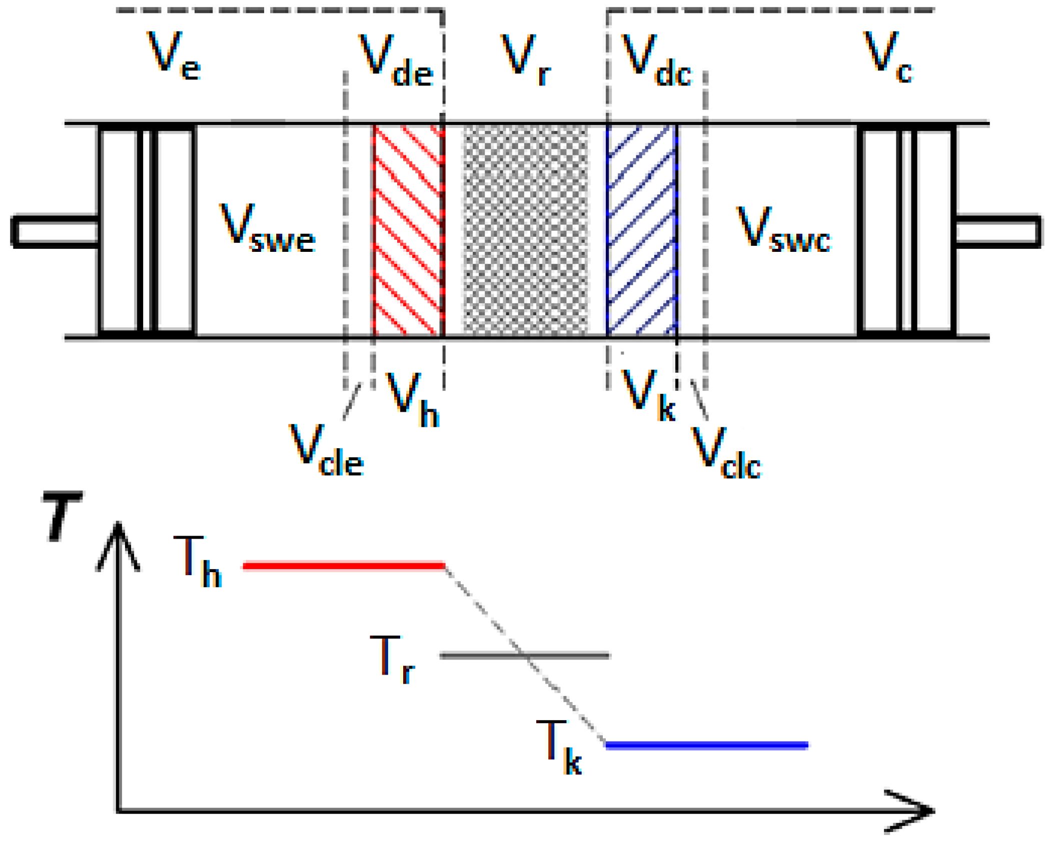
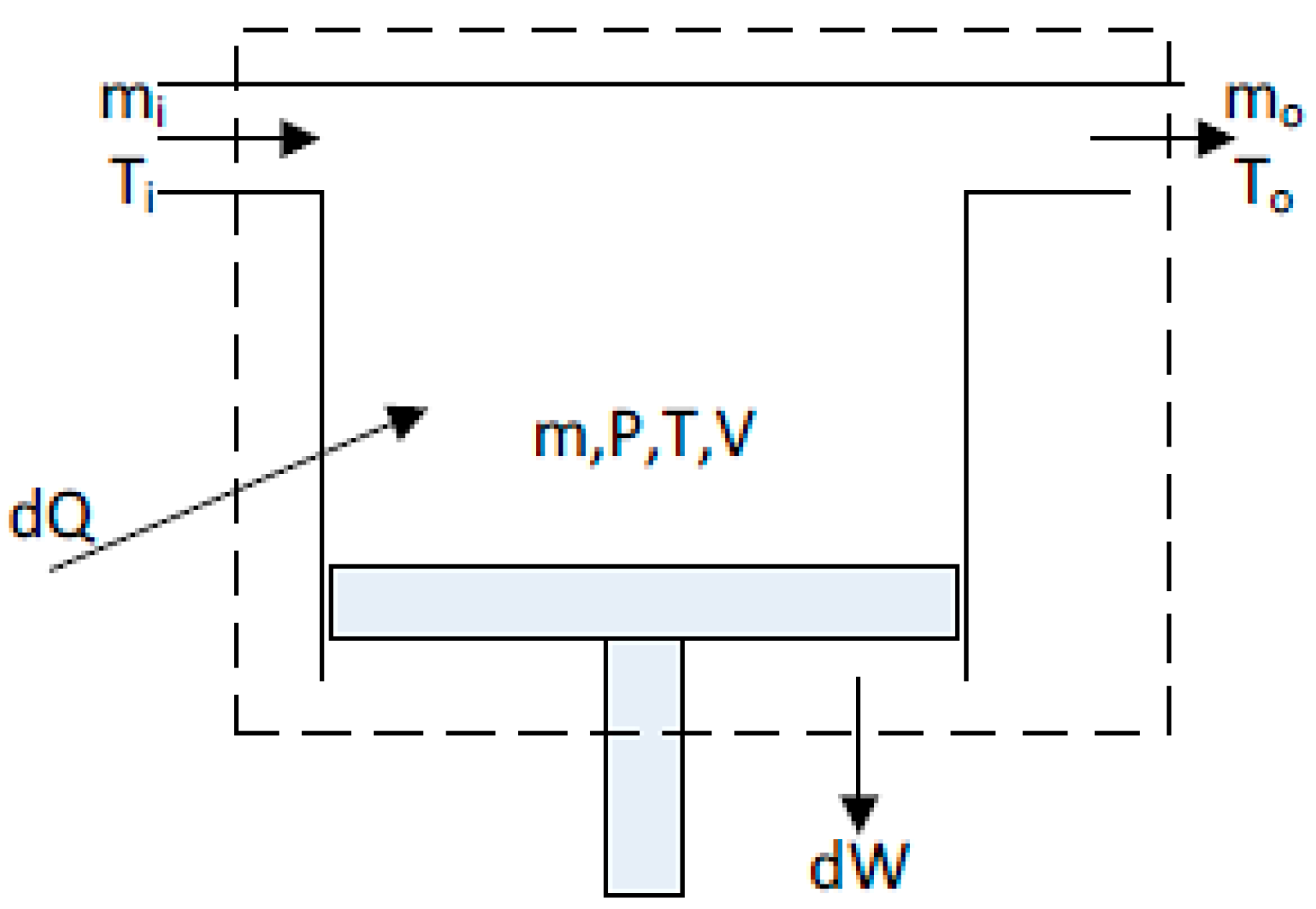
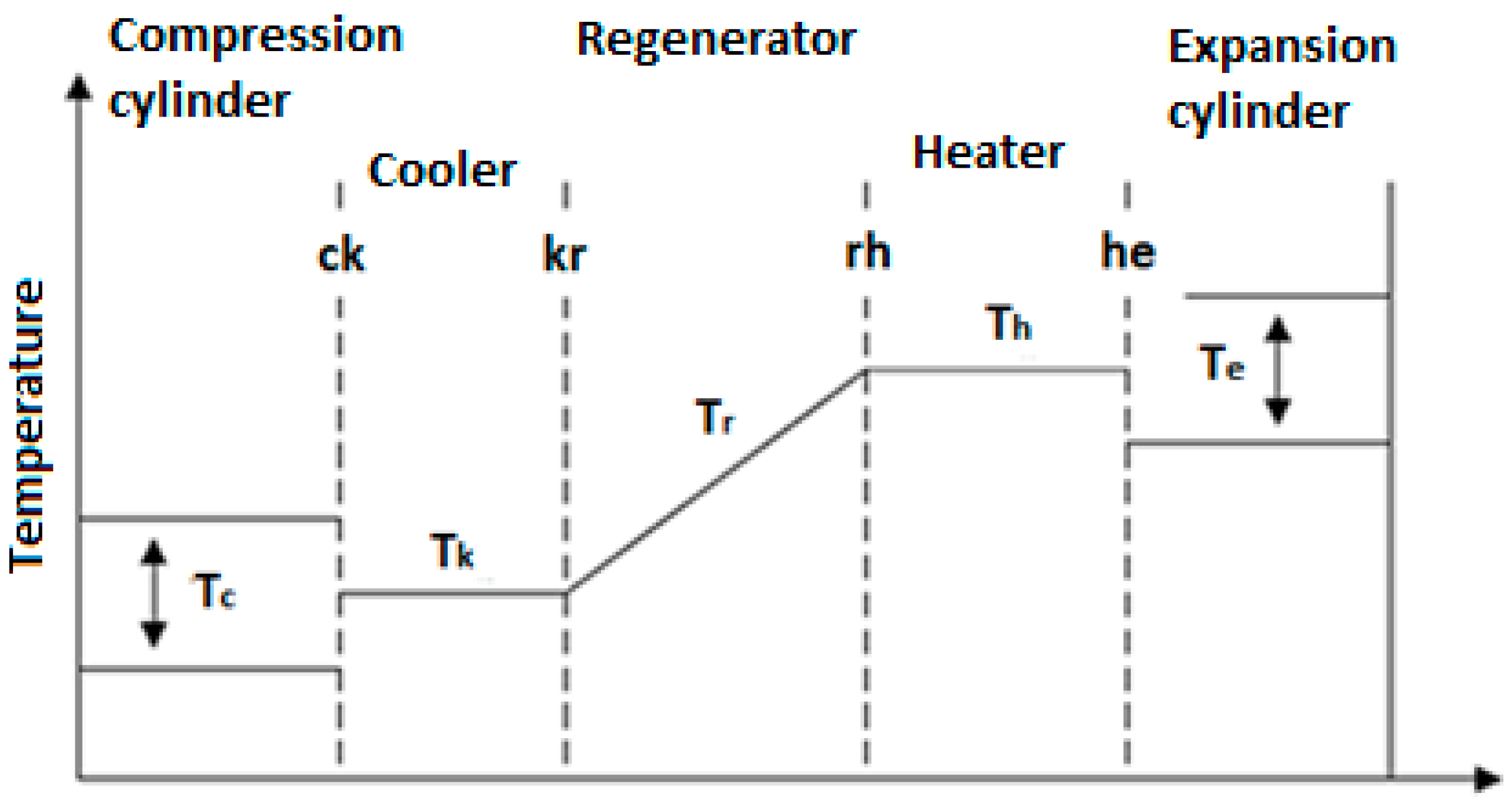
2. Numerical Model
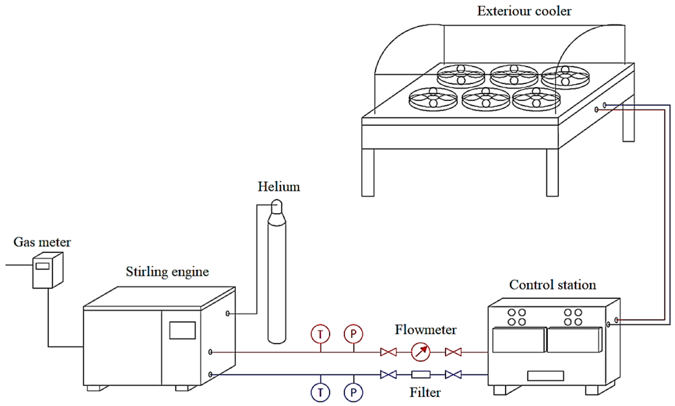
3. Experimental Measurements
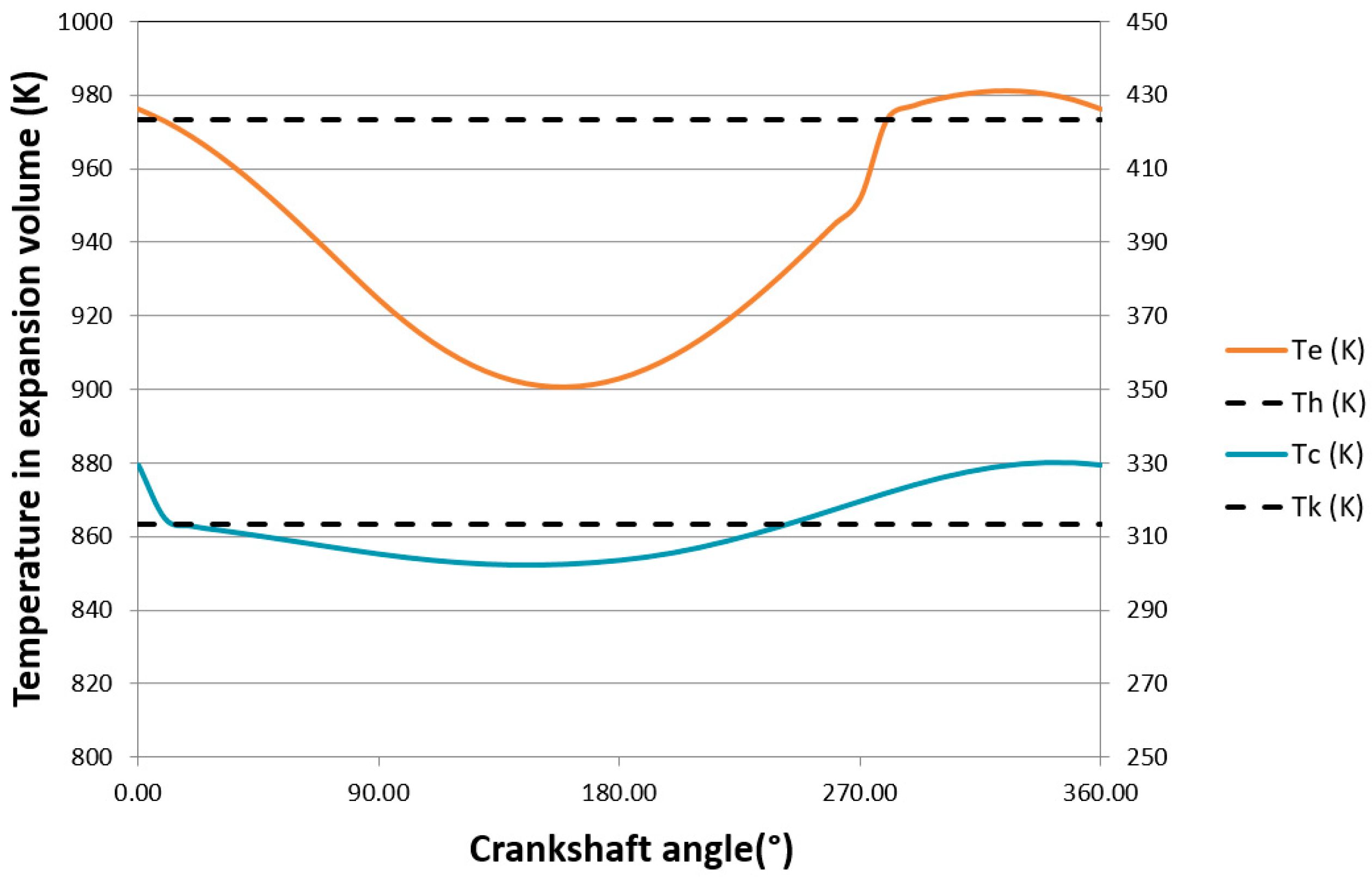
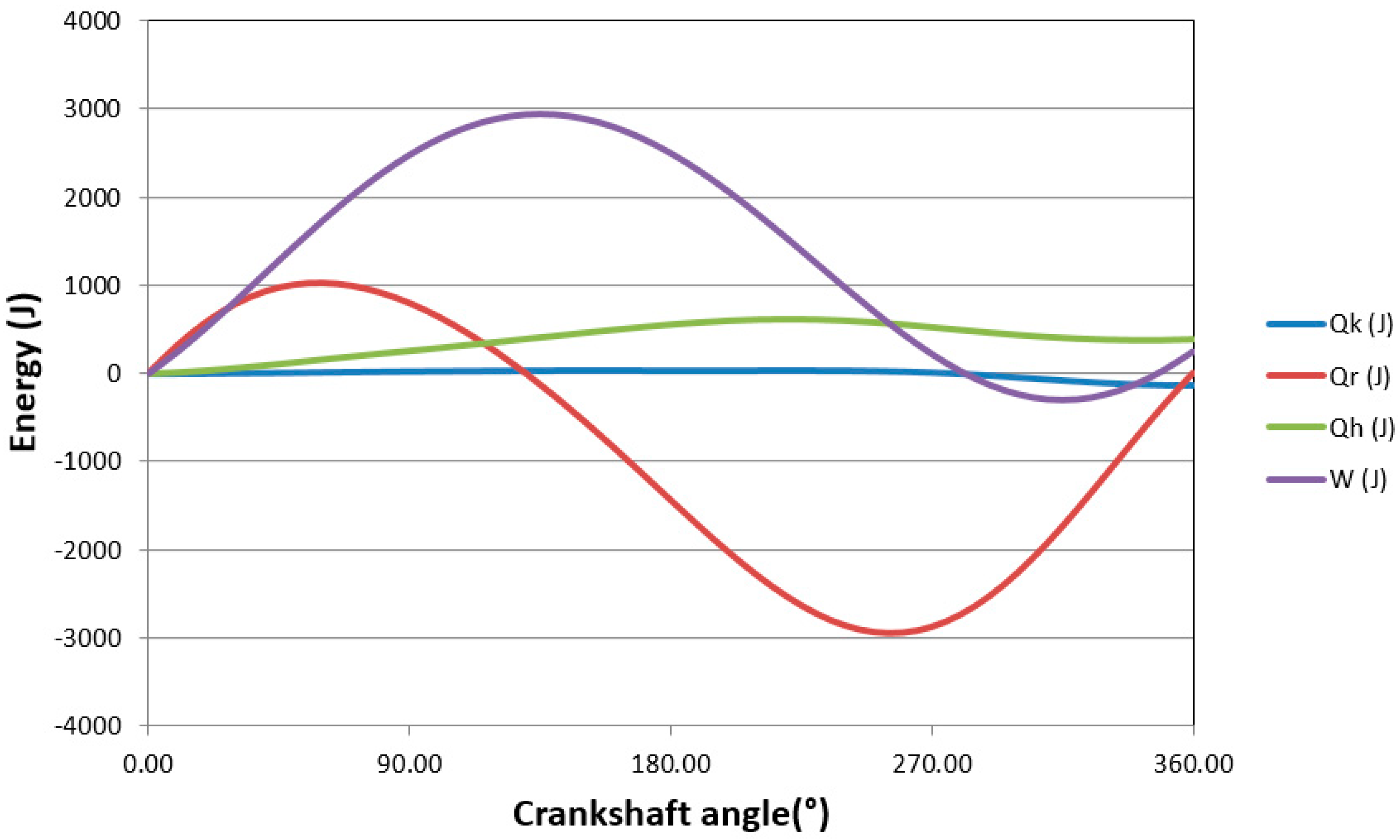
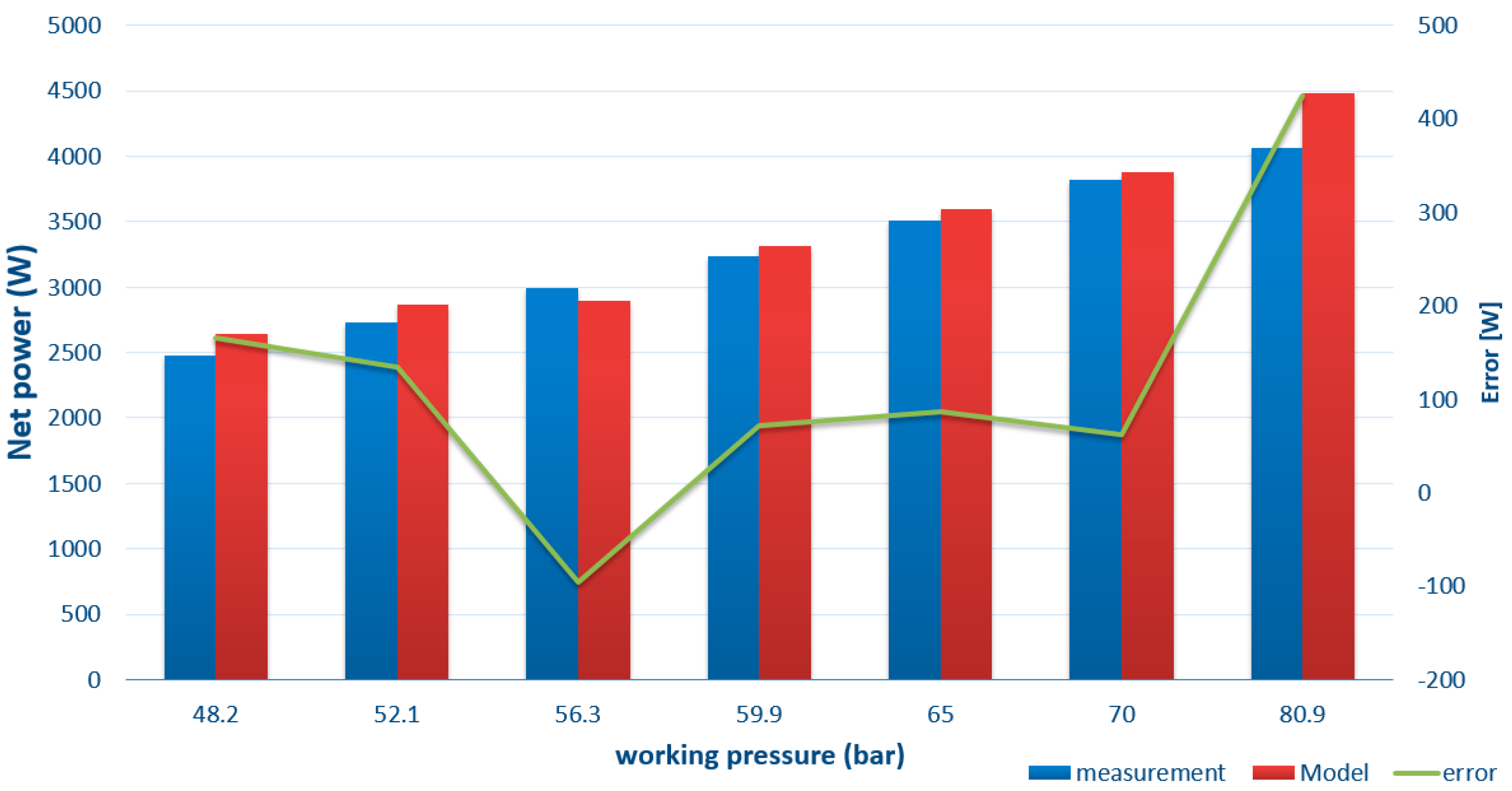
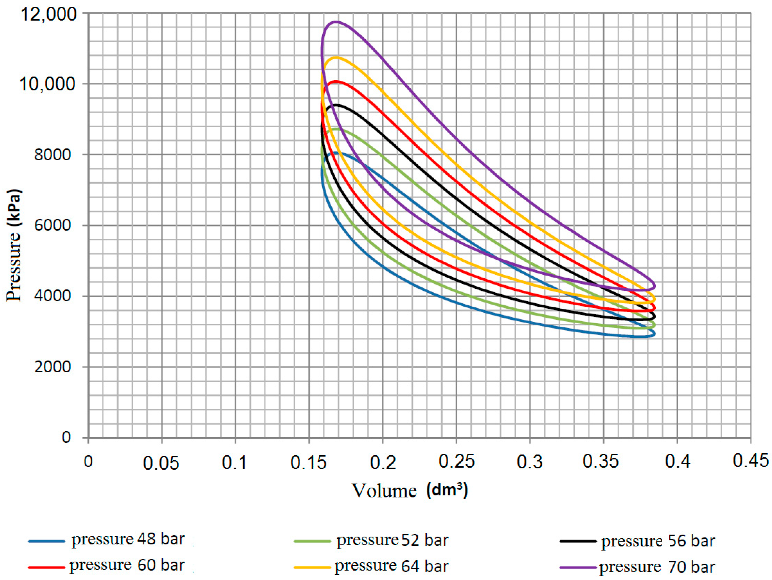
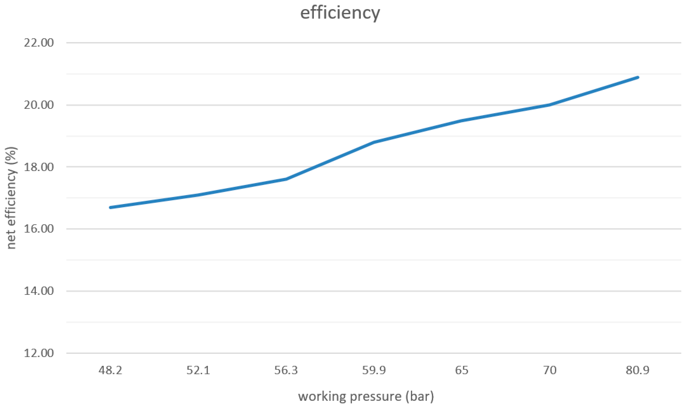
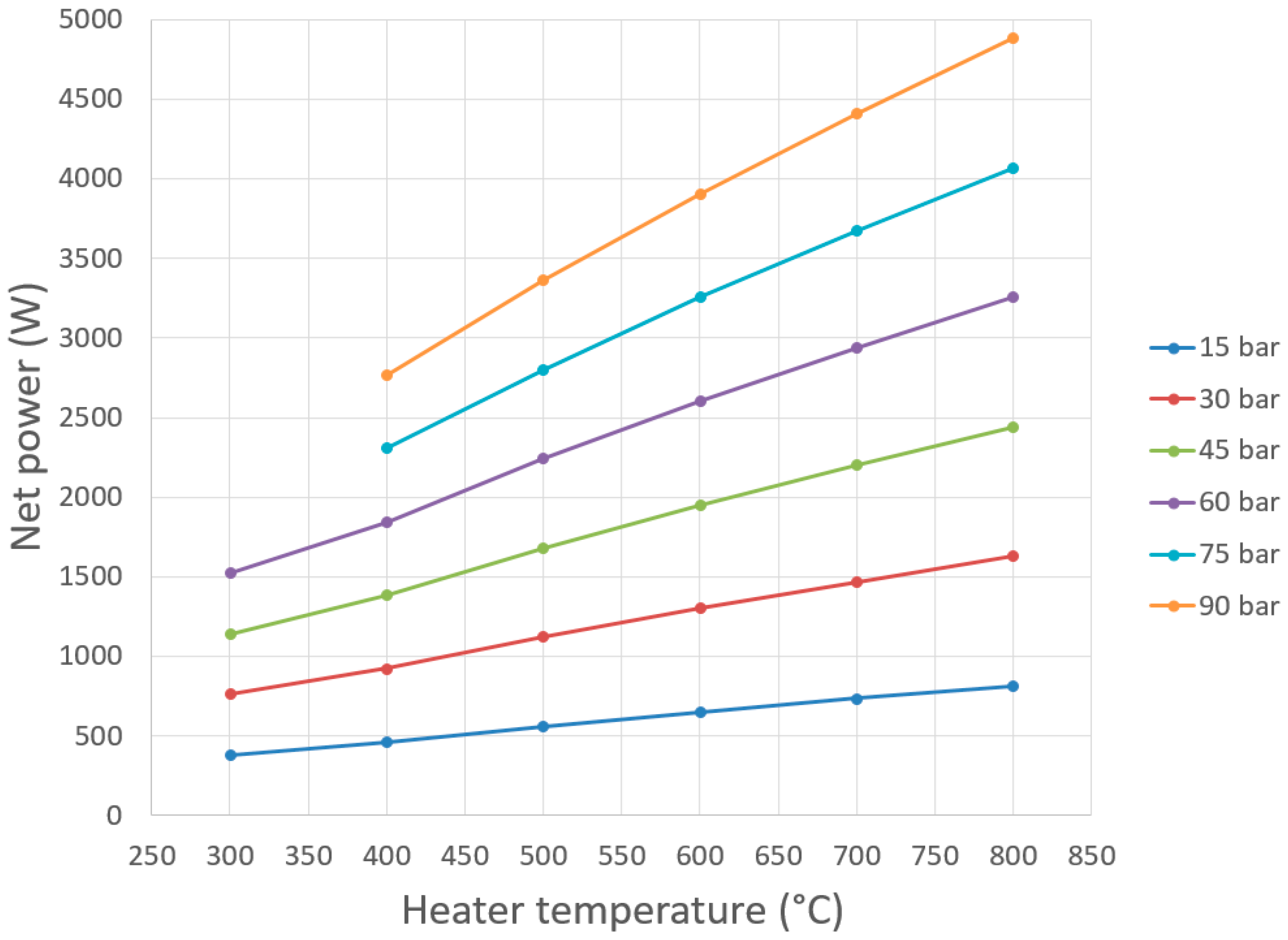
4. Results
5. Discussion
6. Conclusions
Author Contributions
Funding
Conflicts of Interest
Nomenclature, Abbreviations
| Symbol | Unit | Description |
| m | (kg) | working gas mass |
| (kg) | mass flow | |
| M | (kg) | total weight of the engine working medium |
| Q | (J) | heat added or removed |
| T | (K) | temperature |
| V | (m) | volume |
| W | (J) | work |
| Vswc | (m3) | compression cylinder displacement |
| Vswe | (m3) | expansion cylinder displacement |
| (kg/s) | mass flow through heater to expansion cylinder interface | |
| (kg/s) | mass flow through compression cylinder to cooler interface | |
| (kg/s) | mass flow through cooler to regenerator interface | |
| (kg/s) | mass flow through regenerator to heater interface | |
| (kg/s) | mass flow entering the control volume | |
| (kg/s) | mass flow exiting the control volume | |
| Index | ||
| c | compression volume, cylinder | |
| e | expansion volume, cylinder | |
| h | heater | |
| k | cooler, cooling volume | |
| r | regenerator |
References
- Holland, D. An Introduction to Stirling-Cycle Machine, Stirling-Cycle Research Group; Department of Mechanical Engineering, University of Canterbury: Christchurch, New Zealand, 2012. [Google Scholar]
- Renzi, M.; Brandoni, C. Study and application of a regenerative Stirling cogeneration device based on biomass combustion. Appl. Therm. Eng. 2014, 67, 341–351. [Google Scholar] [CrossRef]
- Invernizzi, C.M. Closed Power Cycles; Springer: London, UK, 2013; ISBN 978-1-4471-5140-1. [Google Scholar]
- Thombare, D.G.; Verma, S.K. Technological development in the Stirling cycle engines. Renew. Sustain. Energy Rev. 2008, 12, 1–38. [Google Scholar] [CrossRef]
- Mcgovern, J.; Cullen, B.; Feidt, M.; Petrescu, S. Validation of a Simulation Model for a Combined Otto and Stirling Cycle Power Plant. Presented at ASME 4th International Conference on Energy Sustainability, Phoenix, AZ, USA, 17–22 May 2010. [Google Scholar]
- Finkelstein, T.; Organ, A.J. Air Engines: The history, Science, and Reality of Perfect Engine; ASME Press: New York, NY, USA, 2001; ISBN-13: 978-07918-0171-0. [Google Scholar]
- Wang, K.; Sanders, R.S.; Dubey, S.; Choo, F.H.; Duan, F. Stirling cycle engines for recovering low and moderate temperature heat: A review. Renew. Sustain. Energy Rev. 2016, 62, 89–108. [Google Scholar] [CrossRef]
- Araoz, J.A.; Salomon, M.; Alejo, L.; Fransson, T.H. Numerical simulation for the design analysis of kinematic Stirling engines. Appl. Energy 2015, 159, 633–650. [Google Scholar] [CrossRef]
- Karabulut, H.; Cinar, C.; Ozturk, E.; Yucesu, H. Torque and power characteristics of a helium charged Stirling engine with a lever controlled displacer driving mechanism. Renew. Energy 2010, 35, 138–143. [Google Scholar] [CrossRef]
- Kwankaomeng, S.; Silpsakoolsook, B.; Savangvong, P. Investigation on stability and performance of a free-piston Stirling engine. Energy Procedia 2014, 52, 598–609. [Google Scholar] [CrossRef]
- Cooke-Yarborough, E.H. A Proposal for a Heat-Powered Non-Rotating Electrical Alternator; UKAEA Atomic Energy Research Establishment: Harwell, UK, 1967.
- Martini, W.R. Stirling Engine Design Manual, 2nd ed.; University Press of the Pacific: Honolulu, HI, USA, 2004; ISBN 1-4102-1604-7. [Google Scholar]
- Hirata, K. Schmidt Theory for Stirling Engines; National Maritime Research Institute: Tokyo, Japan, 1997. [Google Scholar]
- Charvát, P.; Klimeš, L.; Pech, O.; Hejčík, J. Solar air collector with the solar absorber plate containing a PCM—Environmental chamber experiments and computer simulations. Renew. Energy 2019, 143, 731–740. [Google Scholar]
- Nemec, P.; Caja, A.; Malcho, M. Mathematical Model for Heat Transfer Limitations of Heat Pipe. Math. Comput. Model. 2013, 57, 126–136. [Google Scholar] [CrossRef]
- Chen, L.; Li, J.; Sun, F. Optimal temperatures and maximum power output of a complex system with linear phenomenological heat transfer law. Therm. Sci. 2009, 13, 33–40. [Google Scholar] [CrossRef]
- Hosseinpour, J.; Sadeghi, M.; Chitsaz, A.; Ranjbar, F.; Rosen, M.A. Exergy assessment and optimization of a cogeneration system based on a solid oxide fuel cell integrated with a Stirling engine. Energy Convers. Manag. 2017, 143, 448–458. [Google Scholar] [CrossRef]
- Urieli, I.; Berchowitz, D.M. Stirling Cycle Engine Analysis; Taylor & Francis: Ann Arbor, MI, USA, 1984; 256p, ISBN 0852744358. [Google Scholar]
- Ferreira, A.C.; Nunes, M.L.; Teixeira, J.C.; Martins, L.A.; Teixeira, S.F. Thermodynamic and economic optimization of a solar-powered Stirling engine for micro-cogeneration purposes. Energy 2016, 111, 1–17. [Google Scholar] [CrossRef]
- Chen, W.L.; Wong, K.L.; Chen, H.E. An experimental study on the performance of the moving regenerator for a gamma-type twin power piston Stirling engine. Energy Convers. Manag. 2014, 77, 118–128. [Google Scholar] [CrossRef]
- Ipci, D.; Karabulut, H. Thermodynamic and dynamic analysis of an alpha type Stirling engine and numerical treatment. Energy Convers. Manag. 2018, 169, 34–44. [Google Scholar] [CrossRef]
- Cheng, C.-H.; Yu, Y.-J. Numerical model for predicting thermodynamic cycle and thermal efficiency of a beta-type Stirling engine with rhombic-drive mechanism. Renew. Energy 2010, 35, 2590–2601. [Google Scholar] [CrossRef]
- Cheng, C.-H.; Tan, Y.-H. Numerical optimization of a four-cylinder double-acting stirling engine based on non-ideal adiabatic thermodynamic model and scgm method. Energies 2020, 13, 2008. [Google Scholar] [CrossRef]
- Brestovič, T.; Carnogurska, M.; Prihoda, M.; Lukac, P.; Lázár, M.; Jasminská, N.; Dobáková, R. Diagnostics of hydrogen-containing mixture compression by a two-stage piston compressor with cooling demand prediction. Appl. Sci. 2018, 8, 625. [Google Scholar] [CrossRef]
- Világi, F.; Knížat, B.; Mlkvik, M.; Urban, F.; Olšiak, R.; Mlynár, P. Mathematical model of steady flow in a helium loop. Mech. Ind. 2019, 20, 704–712. [Google Scholar]
- Ahmed, F.; Hulin, H.; Khan, A.M. Numerical modeling and optimization of beta-type Stirling engine. Appl. Therm. Eng. 2019, 149, 385–400. [Google Scholar] [CrossRef]
- Ni, M.; Shi, B.; Xiao, G.; Peng, H.; Sultan, U.; Wang, S.; Luo, Z.; Cen, K. Improved Simple Analytical Model and experimental study of a 100W β-type Stirling engine. Appl. Energy 2016, 169, 768–787. [Google Scholar] [CrossRef]
- Bataineh, K.M. Numerical thermodynamic model of alpha-type Stirling engine. Case Stud. Therm. Eng. 2018, 12, 104–116. [Google Scholar] [CrossRef]
- Rogdakis, E.D.; Antonakos, G.D.; Koronaki, I.P. Thermodynamic analysis and experimental investigation of a Solo V161 Stirling cogeneration unit. Energy 2012, 45, 503–511. [Google Scholar] [CrossRef]
- Westerberg, J. An Experimental Evaluation of Low Caloric Value Gaseous Fuels as a Heat Source for Stirling Engines. Master’s Thesis, Chalmers University of Technology, Goteborg, Sweden, March 2014. [Google Scholar]
- Wackerly, D.; Mendenhall, W.; Scheaffer, R.L. Mathematical Statistics with Applications, 7th ed.; Thomson Brooks/Cole: Pacific Grove, CA, USA, 2008; ISBN-13: 978-0495110811. [Google Scholar]
- Sarkar, J.; Rashid, M. Visualizing Mean, Median, Mean Deviation, and Standard Deviation of a Set of Numbers. Am. Stat. 2016, 70, 304–312. [Google Scholar] [CrossRef]
- Pobočíková, I.; Sedliačková, Z.; Michalková, M. Application of Four Probability Distributions for Wind Speed Modeling. Procedia Eng. 2017, 192, 713–718. [Google Scholar] [CrossRef]


| Engine Manufacturer | Mean Pressure (MPa) | Heater Temperature (°C) | Power (kW) | Efficiency (%) |
|---|---|---|---|---|
| United Stirling [8] | 14.5 | 691 | 35 | 30 |
| Philips [7] | 14.2 | 649 | 23 | 38 |
| GM GPU-3 [8] | Up to 6.9 | 816 | 8.1 | 39 |
| Farwell [8] | 0.1 | 594 | 0.1 | 16.9 |
| Karabulut et al. [9] | 0.4 | 260 | 0.183 | N/A |
| Kwankaomeng [10] | 0.1 | 150 | 0.1 | 5.6 |
| Cooke-Yarborough [11] | N/A | 292 | 0.107 | 13.7 |
| Solo Stirling [12] | N/A | Min. 540 | 7.3 | 25.4 |
| WhisperGen [wikipedia] | N/A | Min. 550 | Up to 1 kW | 11 |
| Viessmann Vitotwin [viessmann.de] | N/A | Min. 500 | Up to 1 kW | 30 |
| Cleanergy [12] | 1.5–9 | N/A | 2–9 | 25 |
| Working Pressure (bar) | Electric Output—Average Value (W) | Efficiency (%) | Standard Deviation of the Arithmetic Mean Value Estimation (W) |
|---|---|---|---|
| 48.2 | 2480 | 16.7 | ±6.5 |
| 52.1 | 2730 | 17.1 | ±4.8 |
| 56.3 | 2990 | 17.6 | ±5.8 |
| 59.9 | 3240 | 18.8 | ±4.1 |
| 65 | 3510 | 19.5 | ±4.9 |
| 70 | 3820 | 20.0 | ±5.0 |
| 80.9 | 4060 | 20.9 | ±5.7 |
© 2020 by the authors. Licensee MDPI, Basel, Switzerland. This article is an open access article distributed under the terms and conditions of the Creative Commons Attribution (CC BY) license (http://creativecommons.org/licenses/by/4.0/).
Share and Cite
Durcansky, P.; Nosek, R.; Jandacka, J. Use of Stirling Engine for Waste Heat Recovery. Energies 2020, 13, 4133. https://doi.org/10.3390/en13164133
Durcansky P, Nosek R, Jandacka J. Use of Stirling Engine for Waste Heat Recovery. Energies. 2020; 13(16):4133. https://doi.org/10.3390/en13164133
Chicago/Turabian StyleDurcansky, Peter, Radovan Nosek, and Jozef Jandacka. 2020. "Use of Stirling Engine for Waste Heat Recovery" Energies 13, no. 16: 4133. https://doi.org/10.3390/en13164133
APA StyleDurcansky, P., Nosek, R., & Jandacka, J. (2020). Use of Stirling Engine for Waste Heat Recovery. Energies, 13(16), 4133. https://doi.org/10.3390/en13164133