Updated Typical Weather Years for the Energy Simulation of Buildings in Mediterranean Climate. A Case Study for Sicily

Abstract

Building energy simulations are normally run through Typical Weather Years (TWYs) that reflect the average trend of local long-term weather data. This paper presents a research aimed at generating updated typical weather files for the city of Catania (Italy), based on 18 years of records (2002–2019) from a local weather station. The paper reports on the statistical analysis of the main recorded variables, and discusses the difference with the data included in a weather file currently available for the same location based on measurements taken before the 1970s but still used in dynamic energy simulation tools. The discussion also includes a further weather file, made available by the Italian Thermotechnical Committee (CTI) in 2015 and built upon the data registered by the same weather station but covering a much shorter period. Three new TWYs are then developed starting from the recent data, according to well-established procedures reported by ASHRAE and ISO standards. The paper discusses the influence of the updated TWYs on the results of building energy simulations for a typical residential building, showing that the cooling and heating demand can differ by 50% or even 65% from the simulations based on the outdated weather file.

1. Introduction

The energy consumption in buildings, which is in large part due to heating, ventilation, and air-conditioning, covers a high share of the overall energy balance worldwide. According to the International Energy Agency (IEA), construction and operation of buildings accounted for 36% of the global final energy use and 39% of the energy-related CO₂ emissions in 2017 [1]. In particular, the energy use in urban areas amounts to over two thirds of the world’s energy consumption and is responsible for more than 70% of the global CO₂ emissions [2].

Then, in light of the rising concern towards environmental issues, and in accordance with the growing number of national and international regulations aiming at a severe reduction in the depletion of non-renewable primary energy sources, the need of detailed studies concerning the energy behavior of buildings has recently become strongly felt.

To this aim, software tools for dynamic energy simulation of buildings are nowadays commonly available and widely used by researchers, engineers, and others involved in the design and optimization of the energy performance of buildings. Indeed, these tools allow a detailed evaluation of both the time-dependent thermal loads and the indoor thermal comfort conditions, while taking into account the inertial effects due to the thermal capacity of the building enclosure [3].

However, reliable energy simulations depend strongly on the availability of accurate weather data. Most building energy simulation tools make use of weather files based on a Typical Weather Year (TWY), that is to say a full year of typical local hourly weather data generated by statistically averaging long-term weather measurements, issued by weather stations commonly placed in peripheral or rural zones. The use of TWYs has gained wide consensus in the building simulation community because they depict average climate trends, which in turn are related to the thermal behavior of a building in average conditions, while disregarding extreme weather events [4].

Now, the users of a building energy simulation tool should be aware that several drawbacks may arise when using a TWY as an input to energy simulation. Indeed, a TWY may not reflect the actual weather conditions experienced by a building in a specific site due to year-to-year climate fluctuations: Hence, a TWY does not account for the yearly variations in the energy needs, which would only be highlighted through a multi-year energy simulation process [5,6], nor can it be reliably used to calculate the peak loads occurring in design conditions [3]. Moreover, many available TWYs are out-of-date, meaning that they are based on weather measurements dating back several decades. This is likely to affect the calculated energy needs of a building, in a range between 5% and 10% according to Wang et al. [7], as well as the predicted indoor thermal comfort [8]; similar conclusions were drawn by Pernigotto et al., who found out that even the energy rating of a building can be influenced by the use of inappropriate or outdated weather files [9]. Lou et al. suggest that the weather files should be updated every 12 years [10]. These results question the suitability of many existing—and universally used—TWYs for the accurate prediction of heating and cooling loads of buildings.

In Italy, most of the currently available weather files derive from hourly measurements taken in the period 1951–1970. These data were then elaborated in the framework of the national research project entitled “Progetto Finalizzato Energetica” in 1979, and led to the release of the Italian climatic data collection “Gianni De Giorgio” (IGDG): This is a database populated by weather information from 68 weather stations evenly distributed in the national territory, later processed in order to be used in different simulation tools [11]. An update of many weather files was released in 2015 by the Italian Thermotechnical Committee (CTI), which enlarged the original domain by considering a set of 110 localities [12]. However, for many of the available locations the period of measurement is short (i.e., less than 10 years), and this may undermine the reliability of these weather files in the field of building energy simulation. It is then undeniable that new TWYs are needed based on more recent and extensive weather data.

Under these premises, this paper presents recent hourly weather data recorded from 2002 to 2019 by a weather station owned by the Sicilian Agrometeorological Information System (SIAS) in Catania (Italy). A statistical analysis compares this dataset with the old IGDG dataset available for the same city and currently largely used by the local research community thus underlining the main differences. Then, after a literature review regarding the creation of typical years in different countries worldwide, as well as their effect on the outcomes of energy simulation tools (Section 2), in Section 3 the paper describes three well-established procedures commonly used to extract a typical year from a set of weather data, which are then used to generate three new TWYs from the SIAS dataset. The aim is not only the development of the updated TWYs, but also a critical comparison of the different procedures and their outcomes, while also discussing the need to perform some pre-processing activities for data quality check and gap filling (Section 4). Finally, the paper investigates the influence of these updated weather files on the results of building energy simulations for a typical residential building located in the city of Catania.

2. Literature Review on Typical Weather Years for Energy Simulation of Buildings

A literature review on this topic shows that many different procedures have been established to extract a typical weather year from a multi-year weather dataset. However, in the field of energy simulation of buildings and their technical systems, three procedures are mainly used:

• the procedure designed by Hall et al. [13] at Sandia Laboratories in 1978, leading to the original format called Typical Meteorological Year (TMY) and then slightly modified by the National Renewable Energy Laboratory (NREL) into the more recent formats called TMY2 in 1995 [14] and TMY3 in 2005 [15];
• the ASHRAE procedure, leading to the IWEC format (International Weather for Energy Calculations), respectively in its original version of 2002 [16] and the updated IWEC2 version of 2014 [17];
• the procedure introduced by the ISO 15927-4 Standard in 2005 [18].

Other procedures proposed in the literature, such as the Festa-Ratto method [19] and the Danish method [20], did not find wide diffusion in the scientific community and are seldom used. In Canada, the weather files are instead created according to the Canadian Weather Year for Energy Calculation (CWEC) method [21].

In any case, these procedures aim to extract—for each calendar month—a typical month from all the years of observation. The twelve selected typical months, which do not necessarily belong to the same year, are then concatenated to create a typical year. This approach must not be confused with the generation of a Typical Reference Year (TRY) introduced by ASHRAE in the 1970s [22], where an entire year—with its 8760 h series of data—is selected out of the multi-year measurements.

The three previously listed methods differ from each other in various aspects, such as the list of weather parameters included in the selection process and the weights that are attributed to them. These weights are intended to describe the relative importance attributed to each weather parameter, and should in principle be coherent with the final purpose of the selected typical weather year. As an example, the original TMY was firstly developed for the simulation of solar energy systems, and for this reason a very high weight is attributed to the solar irradiation, while other parameters (wind speed, relative humidity) have a minor role [13]. Other differences concern the source of the weather data: In some cases, the values of solar irradiation (either global horizontal or direct normal) do not derive from actual measurements, but they originate from the application of suitable mathematical models. More details about the methodological differences among the selection procedures are provided in Section 3.1.

Table 1. Papers dealing with the typical weather year (TWY) generation and their effect on building energy simulation.

Authors	Ref.	Year	Selection Procedure				Number of Sites	Energy Simulation	Country
			TMY	IWEC	ISO	Other
Argiriou et al.	[23]	1999	x	-	-	x	1	x	Greece
Kalogirou	[30]	2003	x	-	-	-	1	-	Cyprus
Sawaqed et al.	[41]	2005	x	-	-	-	7	-	Oman
Levermore and Parkinson	[33]	2006	-	x	-	-	14	-	UK
Chan et al.	[24]	2006	x	x	-	-	1	-	Hong Kong
Rahman and Dewsbury	[40]	2007	-	-	x	-	1	-	Malaysia
Skeiker	[35]	2007	x	-	-	x	1	x	Syria
Lhendup and Lhendup	[44]	2007	-	-	-	x	4	-	Australia
Yang et al.	[52]	2007	x	-	-	-	35	-	China
Janjai and Deeyai	[43]	2009	x	-	-	x	4	x	Thailand
David et al.	[51]	2010	-	-	-	x	23	-	Worldwide
Ebrahimpour and Maerefat	[42]	2010	x	-	-	-	1	-	Iran
Lee et al.	[32]	2010	-	x	-	-	7	-	South Korea
Jiang	[28]	2010	x	-	-	-	8	-	China
Oko and Ogoloma	[34]	2011	x	-	-	-	1	-	Nigeria
Bhandari et al.	[37]	2012	x	-	-	-	1	x	USA
Sorrentino et al.	[49]	2012	x	-	x	x	1	x	Italy
Kalamees et al.	[29]	2012	-	-	x	-	4	x	Finland
Ohunakin et al.	[45]	2013	x	-	-	-	5	-	Nigeria
Ohunakin et al.	[53]	2014	x	-	-	-	1	-	Nigeria
Pernigotto et al.	[9]	2014	-	-	x	-	5	x	Italy
Pernigotto et al.	[48]	2014	x	-	x	-	5	x	Italy
Bre and Fachinotti	[27]	2016	-	x	-	-	15	x	Argentina
Chan	[25]	2016	x	x	-	-	1	x	Hong Kong
Zang et al.	[46]	2016	x	-	-	x	35	-	China
Kulesza	[31]	2017	x	-	x	-	1	-	Poland
Yilmaz and Ekmekci	[36]	2017	x	-	-	-	81	-	Turkey
Pernigotto et al.	[47]	2017	-	-	x	-	2	x	Italy
Hosseini et al.	[38]	2017	-	-	-	x	1	x	Canada
Kim et al.	[50]	2017	x	-	x	-	18	x	South Korea
Arima et al.	[54]	2017	-	-	-	x	1	x	Japan
Crawley and Lawrie	[39]	2019	x	-	-	x	5	x	USA, UK
Siu and Liao	[26]	2020	-	-	-	x	1	x	Canada

reports a list of papers dealing with the generation of typical weather years for studying the energy performance of buildings and their energy systems, published in the last twenty years either on peer-reviewed journals or on conference proceedings [9,23,24,25,26,27,28,29,30,31,32,33,34,35,36,37,38,39,40,41,42,43,44,45,46,47,48,49,50,51,52,53,54]. The original TMY format has been adopted in 63% of the papers, and is by far the most commonly used, followed by the ISO procedure (23%) and the IWEC procedure (14%).

A few studies adopt other official procedures, such as the Festa-Ratto method and the Danish method, or even try to develop new procedures implemented in TRNSYS [44] or C++ [51]. All studies conducted in Canada rely on the CWEC procedure [26,38]. Finally, around 47% of the reported papers discusses the influence of the newly generated weather files on the results of building energy simulations, when compared with outdated weather files.

The first message emerging from this literature review is that a weather file built upon a too short weather dataset (i.e., below 10 years) is likely to produce misleading results [9]. Actually, this problem affects many of the recent weather files prepared by CTI for Italian locations, including Catania: Then, these CTI files do require further development based on more years of measurements.

As far as the different selection procedures are concerned, it is not possible to identify a single procedure that always performs better than the others. Some authors found out that the results of the energy simulations carried out with different typical weather years are similar [25,43], while other authors could find some discrepancies (up to 10%) in the calculation of the annual energy needs [35,37,49], which may also influence the decision-making process during the design stage [47]; however, this outcome depends on the specific building and climate.

Moreover, many authors agree that using a single typical weather year cannot reflect the year-by-year variability in the energy demand of a building. Indeed, this can deviate from the results of a single-year simulation, especially in the winter and for residential uninsulated lightweight buildings [9,23,27], while in the summer the deviation is less evident, unless in largely glazed buildings [9]. In commercial buildings with large flat roofs, the deviation in the seasonal energy demand for cooling may reach 12% [38]. Bevilacqua et al. highlighted that simulated heating and cooling load for a building equipped with a green roof in Southern Italy may vary by around 30% and 15%, respectively, when adopting weather files based on two consecutive actual years [55]. This suggests that further investigation is needed to develop case-dependent weighting sets in order to minimize the distance with the average multi-year simulation results [9,25,29,39,48].

Finally, several authors have underlined that the use of outdated typical years, dating back from the 1990s or even before, causes a significant overestimation in the heating demand of buildings, and a slight underestimation in the cooling demand [26,56,57,58]. This also suggests the need to investigate how weather data can evolve according to different climate scenarios, and to generate suitable TWYs referring to future time horizons. An interesting application of this approach is presented by Vasaturo et al. [59].

3. Methodology

3.1. Procedure for the Identification and Concatenation of the Typical Months

This section describes the methodology followed to build the typical weather years according to the different selection procedures. It is here worth highlighting that the authors made the choice of working only with measured weather data, thus not relying on the adoption of mathematical models for the estimate of the different solar irradiation components. For this reason, and because the SIAS weather station does not measure the direct normal irradiation, the only procedures considered in the paper are those not requiring this parameter through the selection process, that is to say TMY (first original version), IWEC, and ISO 15927.

The procedure for the extraction of Typical Months (TMs) from a long-term observational weather dataset can be summarized in the following sequential steps:

1. 

Selection of the weather parameters for statistical analysis. TMY and IWEC methodologies, building upon the original method by Hall et al. [13], choose the following nine parameters that are considered with daily frequency: Minimum, maximum and mean values of dry bulb air temperature (°C) and dew point temperature (°C), maximum and mean values of the wind speed (m/s), and cumulated global horizontal solar irradiation (Wh/m2). The ISO 15927-4 Standard reduces this set of parameters to only three, i.e., the daily average of dry bulb temperature (°C), relative humidity (%), and global horizontal solar irradiation (Wh/m2). In all cases, the dew point temperature can be replaced by the relative humidity because the two variables can be determined from each other by also using one more independent moist air property (dry bulb temperature) through psychrometrics.

2. 

Construction of the Cumulative Distribution Functions (CDFs) for the selected weather parameters. For every calendar month, the daily values of the selected weather parameters are sorted in ascending order and then used for creating monthly CDFs referred both to the whole period of record (long-term) and to each single year (short-term). CDFs are built according to Equation (1) in the TMY approach, or Equation (2) if the ISO 15927-4 Standard is adopted:

$${\mathrm{S}}_{\mathrm{n}}{\left(\mathrm{x}\right)}_{\mathrm{TMY}}=\{\begin{array}{ll}0& \hspace{1em}\mathrm{for} \mathrm{x}<{\mathrm{x}}_{(1)}\\ \left(\mathrm{k}-0.5\right)/\mathrm{n}& \hspace{1em}\mathrm{for} {\mathrm{x}}_{(\mathrm{k})}\le \mathrm{x}\le {\mathrm{x}}_{(\mathrm{k}+1)}\\ 1& \hspace{1em}\mathrm{for} \mathrm{x}>{\mathrm{x}}_{(\mathrm{n})}\end{array}$$

(1)

$${\mathrm{S}}_{\mathrm{n}}{\left(\mathrm{x}\right)}_{\mathrm{ISO}}=\mathrm{k}\left(\mathrm{x}\right)/\left(\mathrm{n}+1\right)$$

(2)

In the above equations, x is the weather parameter, n is the total number of daily observations for that parameter, k is the order number for each x-value within that calendar month (short-term) or within the whole dataset (long-term). No explicit reference to the previous equations is made in the IWEC method. In this paper, the approach indicated in Equation (1) is followed in the construction of the IWEC typical year.

3. 

Estimate of the closeness of single months’ CDFs to the long-term CDF. For each weather parameter and for each calendar month, the distance between long-term and short-term distributions is evaluated by means of the Finkelstein-Schafer (FS) statistics [60], which is defined as follows for the different procedures:

$$\mathrm{F}{\mathrm{S}}_{\mathrm{TMY}\text{-}\mathrm{IWEC}}\left(\mathrm{x}\right)=\frac{1}{\mathrm{n}}·{\displaystyle \sum _{\mathrm{k}=1}^{\mathrm{n}}{\mathsf{\delta }}_{\mathrm{k}}}=\frac{1}{\mathrm{n}}·{\displaystyle \sum _{\mathrm{k}=1}^{\mathrm{n}}\left|{\mathrm{S}}_{\mathrm{n},\mathrm{year}}\left({\mathrm{x}}_{\mathrm{k}}\right)-{\mathrm{S}}_{\mathrm{n},\mathrm{long}\text{-}\mathrm{term}}\left({\mathrm{x}}_{\mathrm{k}}\right)\right|}$$

(3)

$$\mathrm{F}{\mathrm{S}}_{\mathrm{ISO}}\left(\mathrm{x}\right)={\displaystyle \sum _{\mathrm{k}=1}^n{\mathsf{\delta }}_{\mathrm{k}}}={\displaystyle \sum _{\mathrm{k}=1}^{\mathrm{n}}\left|{\mathrm{S}}_{\mathrm{n},\mathrm{year}}\left({\mathrm{x}}_{\mathrm{k}}\right)-{\mathrm{S}}_{\mathrm{n},\mathrm{long}\text{-}\mathrm{term}}\left({\mathrm{x}}_{\mathrm{k}}\right)\right|}$$

(4)

being n the number of days of that specific month and δ_k the absolute difference between the long-term and the single month CDF values evaluated for every day of the month.

4. 

Weighted sum of the FS statistics and ranking order. Since some weather parameters may be deemed more important than others for building energy simulations, the IWEC and the TMY procedures introduce a weighted sum of the single FS statistics calculated for every parameter, as in Equation (5):

$$\mathrm{W}\mathrm{S}={\displaystyle \sum _{\mathrm{j}=1}^9\mathrm{F}\mathrm{S}\left(\mathrm{j}\right)·{\mathrm{W}}_{\mathrm{j}}}$$

(5)

The weighting factors W_j attributed to each of the nine weather parameters vary with the standards, and are summarized in

Table 2. Non-dimensional weighting factors according to different procedures (T: Dry bulb temperature; RH: Relative humidity; W: Wind speed; GHI: Global horizontal irradiance).

Method	Tmin	Tmax	Tavg	RHmin	RHmax	RHavg	Wmax	Wavg	GHIcum
IWEC	5/100	5/100	30/100	2.5/100	2.5/100	5/100	5/100	5/100	40/100
TMY	1/24	1/24	2/24	1/24	1/24	2/24	2/24	2/24	12/24

. As far as the ISO 15927-4 Standard is concerned, this does not introduce any weighting process, meaning that the same importance is attributed to the three weather parameters considered in this standard.

5. 

Selection of the Typical Month (TM). Here, the IWEC approach implies—for the five months with the lowest WS—the calculation of the monthly mean and median of both the dry bulb temperature and the global horizontal irradiance, and eventually chooses the month closest to the long-term series. On the other hand, the TMY includes a persistence analysis: The candidate months with the longest run and with the highest number of runs either above the 67th long-term percentile or below the 33rd long-term percentile, as well as those with no runs, are excluded; eventually, the top ranked candidate month remaining after the persistence analysis is retained as the Typical Month.

Finally, the ISO 15927-4 Standard selects the TM amongst the three best candidate months coming from step 4 as the one with the lowest deviation of the monthly mean wind speed from the long-term figure.

6.

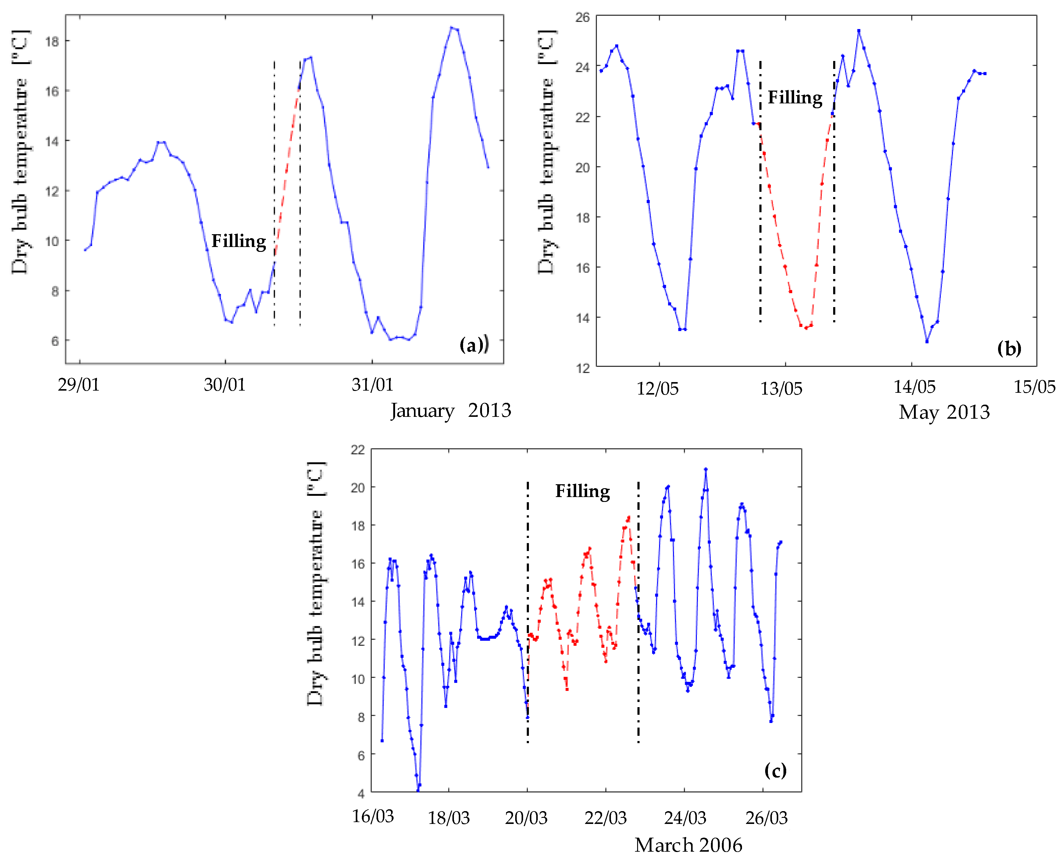
Smoothing discontinuities at month interfaces. Since the 12 selected Typical Months are likely to belong to different years of observation, a smoothing procedure is needed between the last hours of the preceding month and the beginning hours of the following month via curve-fitting or interpolation techniques.

3.2. Preparation of the Weather File in the .epw Format

The final step required to use a typical weather year in a building energy simulation tool consists of arranging the weather data in a suitable format. Amongst the various available formats, this paper relies on the EnergyPlus Weather file (.epw), which can be used with several simulation tools such as EnergyPlus, DesignBuilder, TRNSYS, IES, and ESP-r. This is an ASCII file where, along with a header containing information about the site and the period of record, a series of weather variables are listed with an hourly time step for each Julian day of the year [61].

In addition to the weather variables used to select the TMs, i.e., dry bulb temperature (°C), relative humidity (%), wind speed (m/s), and global horizontal solar irradiance (W/m²), the weather file must contain other physical quantities to correctly estimate the energy and mass exchange between the building and the surroundings. These can be classified as:

• Compulsory parameters: Dew point temperature (°C), atmospheric pressure (Pa), horizontal infrared radiation intensity (W/m²), direct normal irradiance (W/m²), diffuse horizontal irradiance (W/m²), wind direction (degrees from north), and opaque sky cover (tenths of coverage).
• Additional parameters: Snow depth (cm) and liquid precipitation depth (mm).

Actually, once the atmospheric pressure is known (e.g., measured), the dew point temperature depends on the dry bulb temperature and the relative humidity, thus it can be easily calculated by means of psychrometric relations [62].

Building a weather file that can be read by energy simulation programs is then a further demanding step that adds to the generation of the TWY and may even need specific software tools [63].

In this paper, since the direct normal and diffuse horizontal components of the solar irradiance are not measured by the weather station, they are estimated starting from the global horizontal irradiance through the well-established model elaborated by Boland and Ridley [64], which is also the one suggested in the Italian technical norm UNI 10349:1 [65]. Another important parameter to consider is the horizontal infrared radiation of the sky that affects the long-wave radiant exchange of the building. Very few meteorological stations are able to record this quantity, so it has been estimated through Equation (6) [66,67]:

$${\mathrm{G}}_{\mathrm{IR}}={\mathsf{\epsilon }}_{\mathrm{SKY}}·\mathsf{\sigma }·{\mathrm{T}}_{\mathrm{DB}}^4$$

(6)

Here, G_IR is the horizontal infrared radiation intensity in W/m², σ = 5.67 × 10⁻⁸ W/(m² K⁴) is the Stefan-Boltzmann constant, T_DB is the dry bulb temperature recorded at the weather station (in K). The sky emissivity ε_SKY can be calculated through Equation (7) [66,67]:

$${\mathsf{\epsilon }}_{\mathrm{SKY}}=\left[0.787+0.764·\ln \left(\frac{{\mathrm{T}}_{\mathrm{DP}}}{273.15}\right)\right]·\left(1+0.0224·\mathrm{CC}-0.0035·\mathrm{C}{\mathrm{C}}^2+0.00028·\mathrm{C}{\mathrm{C}}^3\right)$$

(7)

where T_DP is the dew point temperature (K) and CC is the opaque sky cover, also known as cloud cover (tenths of sky coverage). Through this approach, the only missing variable is the sky cover.

Since the local weather station does not measure this quantity, the surface-based total cloud cover data have been acquired from the NCDC (National Climatic Data Center) Integrated Surface Database (ISD). Hourly data are freely available at the NCDC website for any user-selected time period and station [68]. Periods of missing data (2 h gaps) were linearly interpolated and adjusted to be consistent with the other meteorological factors.

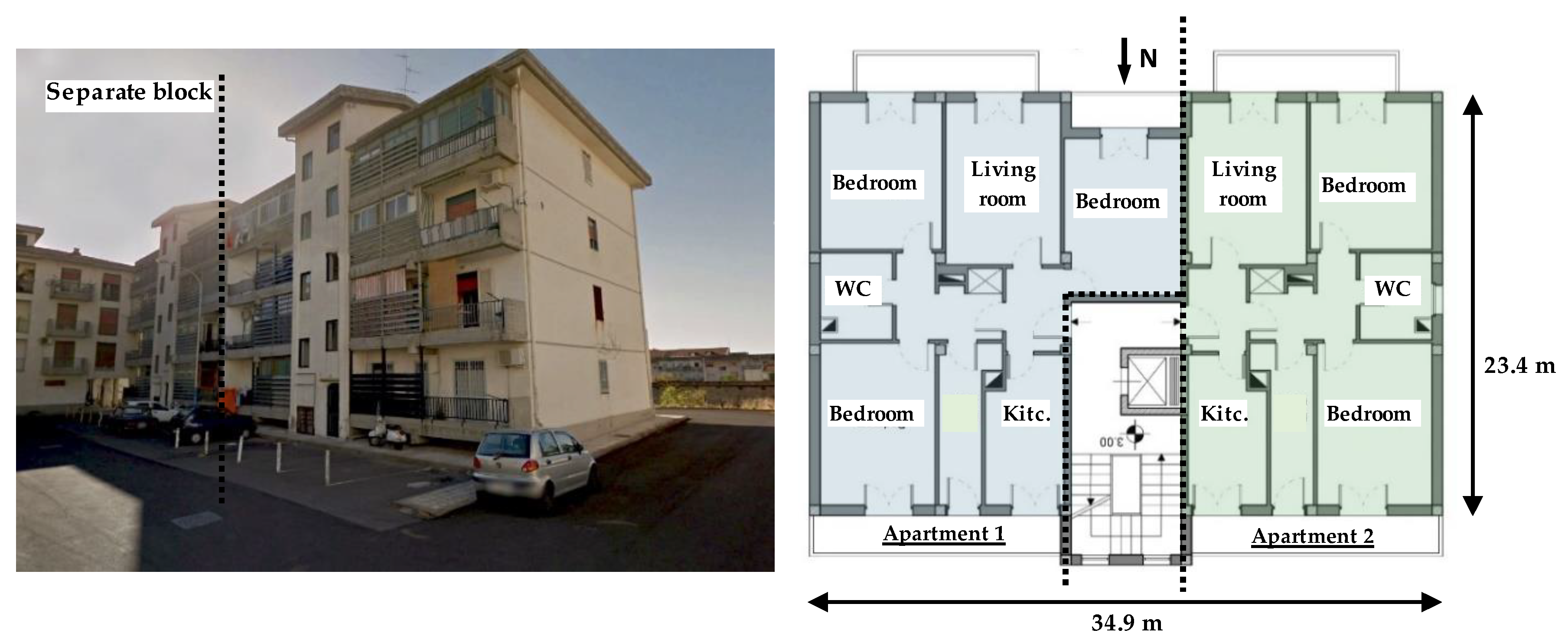
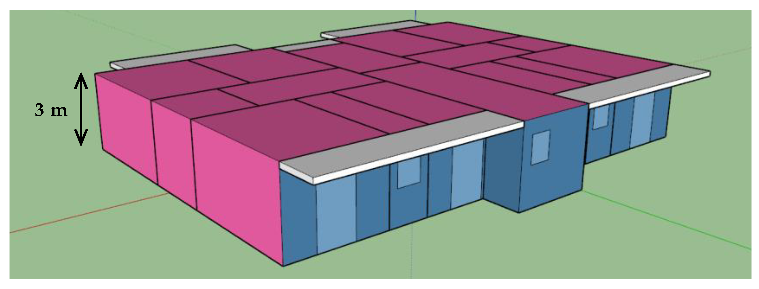
3.3. Case Study Building and Dynamic Energy Simulations

The building chosen as a case study is an apartment block with four storeys located in Catania (Italy), a city with hot and humid climate and sunny days for most of the year. Figure 1 reports a view of the north facade. This residential building has a rectangular shape, and consists of two identical blocks placed side by side; each block has an overall gross floor area of 816 m² and a net floor area of around 725 m². The gross height of each storey is 3 m, while the heated gross volume of the entire building is around 2500 m³.

There are two apartments per floor organized following the same internal distribution and number of rooms: Two or three bedrooms, a kitchen, a living room, two bathrooms, a balcony facing south, and a balcony with a veranda facing north (Figure 1). A stairwell on the north side provides access to the flats at the different floors.

The envelope is quite typical of the Italian buildings constructed in the 1970s, and this makes the building representative of the vast majority of the residential stock in Catania. In particular, the exterior walls are cavity walls with two layers of hollow clay bricks (8 cm on the inner side and 12 cm on the outer side, respectively) and a 10-cm thick air space in between. The intermediate floors and the roof are made of a 20-cm thick lightweight concrete slab, covered with 2-cm thick tiles. Internal partitions consist of 8 cm-thick hollow clay bricks covered with concrete plaster on both sides, while windows are single-glazed with an aluminum frame and no thermal break.

No insulating material is applied to the envelope in its current state. However, the dynamic energy simulations will also consider a variant of the building where the exterior walls are insulated through the addition of a 4 cm outer layer of extruded polyurethane (XPS, λ = 0.030 W m⁻¹ K⁻¹), and the existing windows are replaced by double-glazed low-emissivity windows. This makes it possible to investigate the effect of the different weather files also on a more modern building with better insulation levels that comply with current regulations. The corresponding U-values of the different components, together with the SHGC of the windows, are summarized in

Table 3. Features of the envelope for the selected building.

Building Component	U-Value		SHGC
	Uninsulated Case [W m−2 K−1]	Insulated Case [W m−2 K−1]	Uninsulated Case [–]	Insulated Case [–]
External walls	0.86	0.40	-	-
Slabs	2.72	2.72	-	-
Windows and glazed doors	5.78	1.82	0.862	0.743

.

For energy simulation purposes, the well-known and validated EnergyPlus v.9.0.1 software is used [61]. The simulation only regards one of the two middle-storeys in the Western block that is representative of the average behaviour of the entire building: Accordingly, the adjoining surfaces with the upper and the lower apartments, as well as with the adjacent block, have been treated as adiabatic. The resulting thermal model is shown in Figure 2. In the simulations, the thermal conductivity of the various materials is kept constant; the air cavity is simulated in EnergyPlus as a thermal resistance with no inertial effect. Heat conduction is simulated through the Conduction Transfer Function option in EnergyPlus, with a two-minute time step; the distribution of the solar radiation over the indoor surfaces is computed through the Full Interior and Exterior with Reflections algorithm.

The incoming outdoor air flow rate is supposed to be composed by a fixed value amounting to 0.3 h⁻¹ (average intentional ventilation rate) plus an additional contribution related to air infiltration paths that varies with time according to wind pressure and temperature difference between indoors and outdoors. This contribution is computed through the Effective Leakage Area (ELA) method proposed in the Fundamentals volume of the ASHRAE Handbook [69]. Such an approach first defines a leakage area A_L (in cm²) for every thermal zone as a function of its net volume V_n (in m³) by using the following relation:

$${\mathrm{A}}_{\mathrm{L}}=\frac{{\mathrm{n}}_{\Delta \mathrm{p}}·{\mathrm{V}}_{\mathrm{n}}}{3600}·\sqrt{\frac{\mathsf{\rho }}{2·\Delta \mathrm{p}}}·10000\hspace{1em}[{\mathrm{cm}}^2]$$

(8)

Here, n_Δp is the air exchange rate (in h⁻¹) under a pressure difference Δp. If one assumes Δp = 50 Pa, the corresponding value (n₅₀) can be measured through the blower door test. In the absence of experimental measurements, n₅₀ has been here set to 8 h⁻¹ as suggested by the Italian technical Standard UNI 11300-1:2014 [70] for multi-family apartment blocks with high air permeability. Eventually, the rate of adventitious air flowing through the envelope is computed accounting for both the stack and wind effects by means of Equation (9):

$${\dot{\mathrm{V}}}_{\inf }=\frac{{\mathrm{A}}_{\mathrm{L}}}{1000}·\sqrt{{\mathrm{C}}_{\mathrm{s}}·\Delta \mathrm{T}+{\mathrm{C}}_{\mathrm{w}}·{\mathrm{w}}^2}\hspace{1em}[{\mathrm{m}}^3/\mathrm{s}]$$

(9)

Here, the stack coefficient C_s depends on the number of floors in the buildings, whereas the wind coefficient C_w is a function of the number of floors and the type of surrounding shelters. The selected values (C_s = 1.45 × 10⁻⁴ (L/s)² (cm⁴∙K)⁻¹ and C_w = 2.71 × 10⁻⁴ (L/s)² (cm⁴ m²/s²)⁻¹) are derived from the ASHRAE Handbook [69].

As far as internal gains are concerned, different schedules are defined for the kitchen, bathroom, living room, and bedrooms, but their intensity is kept the same for all the rooms. More in detail, the average occupation rate is 0.04 person/m² with people involved in sedentary activities and releasing 120 W/person indoors (30% of heat is released via the radiant heat exchange). Additionally, internal lights and various electric equipment are lumped together and result in 4 W/m² discharged indoors with a radiant fraction of 20%.

The HVAC system is modeled as an ideal air system, that is to say a fictitious whole-air system with infinite capacity that is always able to instantaneously meet the thermal load. The heating mode runs for 24 h during the winter period (from 1 October to 31 March) at a set point temperature of 20 °C, whereas the cooling mode is in place throughout the day during the summer (from 1 June to 30 September) at a set point temperature of 26 °C. These set point values are chosen according to the provisions of EN 15,251 Standard for Category II of comfort [71].

The simplifications employed in the energy modeling, such as adopting adiabatic surfaces for the bottom and top floors and considering an ideal air system working for 24 h during the heating and cooling seasons, are justified because the aim of these simulations is to highlight the role of weather variables and the consequent differences in the energy needs for space heating and cooling according to different weather datasets only, rather than running detailed building-scale analyses.

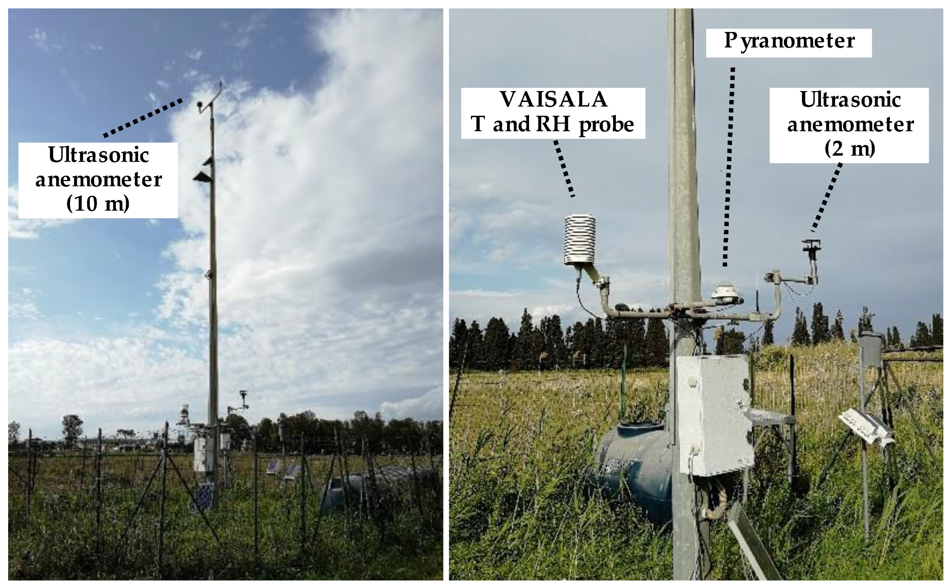
4. The Weather Station

The building energy simulation practice currently relies on the use of weather data collected at rural weather stations for performing hourly annual simulations, thus neglecting—or in the best cases correcting this inaccuracy via morphing procedures [72]—the so called Urban Heat Island (UHI) effect, i.e., the increase in air temperature values in urban settlements if compared to rural ones [73].

For this reason, the weather data used in this study have been recorded by the rural weather station owned by SIAS (Sicilian Agrometeorological Information System), which is located at the following geographical coordinates: 37°26′31″ N, 15°04′04″ E (altitude 10 m asl). Instead, the data included in the IGDG series refer to the weather station next to Fontanarossa airport (37°27′52″ N, 15°03′30″ E, altitude 17 m asl), which is located just 3 km north of the SIAS station. As shown in Figure 3, both weather stations are placed in a rural area, overlooking the sea on the east side and mainly agricultural fields on the north and the south side. The SIAS station has a light industrial and warehousing district to its west side.

The SIAS weather dataset covers a period of 18 years (2002–2019) and contains hourly values of dry bulb temperature (in °C), relative humidity (in %), global horizontal irradiation (in MJ/m²), wind speed (in m/s), wind direction, and atmospheric pressure (in hPa). The dry bulb temperatures were measured from 2002 to 2009 with a MTX-TAM sensor (accuracy ±0.15 °C), whereas in 2010 a Vaisala HMP45 temperature and humidity probe was installed (accuracy ±0.2 °C and ±1% at 20 °C, respectively). The global horizontal irradiation is measured by a Schenk pyranometer type 8102 (accuracy < 10 W/m²). The wind speed and direction are measured by two Gill Windsonic ultrasonic anemometers (accuracy ±2% and ±2°, respectively) placed at 2 and 10 m above ground, as shown in Figure 4.

The collected data were preprocessed and checked for detecting missing or invalid measurements. In particular, the criteria listed in

Table 4. Criteria leading to the identification of invalid measured data.

Dry bulb Temperature	Values outside an acceptable range (−30 ÷ 50 °C) Values exceeding by 50% the 99th percentile Constant values for more than five consecutive h Data with a derivative larger than ±6 °C/h
Relative Humidity	Values outside an acceptable range (0 ÷ 100%) Constant values for more than five consecutive h
Global Horizontal Irradiation	Values outside an acceptable range (0 ÷ 1400 Wh/m2) Positive values after sunset or before sunrise
Wind Speed	Values outside an acceptable range (0 ÷ 50 m/s) Values exceeding by 50% the 99th percentile Constant values for more than five consecutive h

were used to identify invalid measurements.

Table 5. Gaps in the hourly data measured by the SIAS station, before and after the filling procedure.

Year	Jan	Feb	Mar	Apr	May	Jun	Jul	Aug	Sept	Oct	Nov	Dec
2002	744/-	672/-	744/-	720/-	744/-	720/-	517/744	329/744	-/-	528/-	720/-	448/-
2003	-/-	-/-	-/-	-/-	-/-	-/-	-/-	287/744	34/-	-/-	483/720	744/744
2004	348/744	96/672	-/-	-/-	-/-	200/720	-/-	35/-	1/-	-/-	171/-	208/744
2005	41/-	-/-	-/-	1/-	-/-	-/-	-/-	-/-	107/720	2/-	-/-	53/-
2006	124/744	3/-	65/-	1/-	150/744	-/-	-/-	-/-	16/-	199/744	16/-	83/-
2007	1/-	10/-	39/-	5/-	-/-	7/-	-/-	-/-	-/-	8/-	10/-	21/-
2008	1/-	95/672	32/-	-/-	-/-	-/-	33/-	-/-	-/-	-/-	217/720	12/-
2009	40/-	4/-	3/-	-/-	-/-	-/-	-/-	-/-	2/-	11/-	-/-	13/-
2010	221/744	45/-	117/744	269/720	34/-	1/-	17/-	10/-	4/-	1/-	8/-	2/-
2011	2/-	-/-	2/-	-/-	2/-	2/-	-/-	-/-	-/-	-/-	-/-	1/-
2012	1/-	2/-	-/-	1/-	1/-	-/-	-/-	-/-	-/-	1-/-	-/-	-/-
2013	4/-	4/-	-/-	6/-	14/-	-/-	-/-	2/-	-/-	-/-	-/-	-/-
2014	1/-	-/-	-/-	1/-	1/-	-/-	-/-	-/-	-/-	-/-	-/-	25/-
2015	2/-	-/-	-/-	-/-	-/-	-/-	-/-	2/-	2/-	-/-	-/-	-/-
2016	-/-	-/-	-/-	-/-	-/-	1/-	-/-	-/-	-/-	-/-	-/-	2/-
2017	-/-	1/-	-/-	1/-	-/-	-/-	-/-	-/-	-/-	-/-	3/-	1/-
2018	-/-	-/-	1/-	-/-	-/-	-/-	-/-	-/-	-/-	2/-	-/-	94/-
2019	-/-	-/-	-/-	-/-	1/-	-/-	-/-	-/-	1/-	-/-	-/-	1/-

reports the number of gaps in the hourly data for at least one of the following parameters: Dry bulb temperature, relative humidity, wind speed, and solar irradiation. Those months showing gaps longer than 72 consecutive h were rejected (in bold) and not considered in the further analyses for the typical weather year development, whereas different interpolation methods were used for all gaps up to 72 consecutive h.

In particular, invalid and missing data up to six consecutive h were replaced by using linear interpolation, while gaps between 6 and 72 h were filled by linear interpolation of the measured data having the same position (i.e., hour) in the neighboring days.

Examples of the filling procedure are reported in Figure 5. The filled values were adjusted to preserve nonlinearities and appropriately scaled to match the endpoints of the interpolation interval. Most of the global horizontal irradiation data are missing in 2002: In this case, hourly data for solar irradiation were recovered from the National Aeronautics and Space Administration (NASA), MERRA-2 Project (http://gmao.gsfc.nasa.gov/reanalysis/MERRA-2).

At the end of this section it is worth recalling that the data recorded by the SIAS weather station from 2002 to 2009 have been used by the Italian Thermotechnical Committee (CTI) for the release of a Test Reference Year in 2015. This reference year, which is based on a very short observation period, will be used as a term of comparison in the following.

5. Results

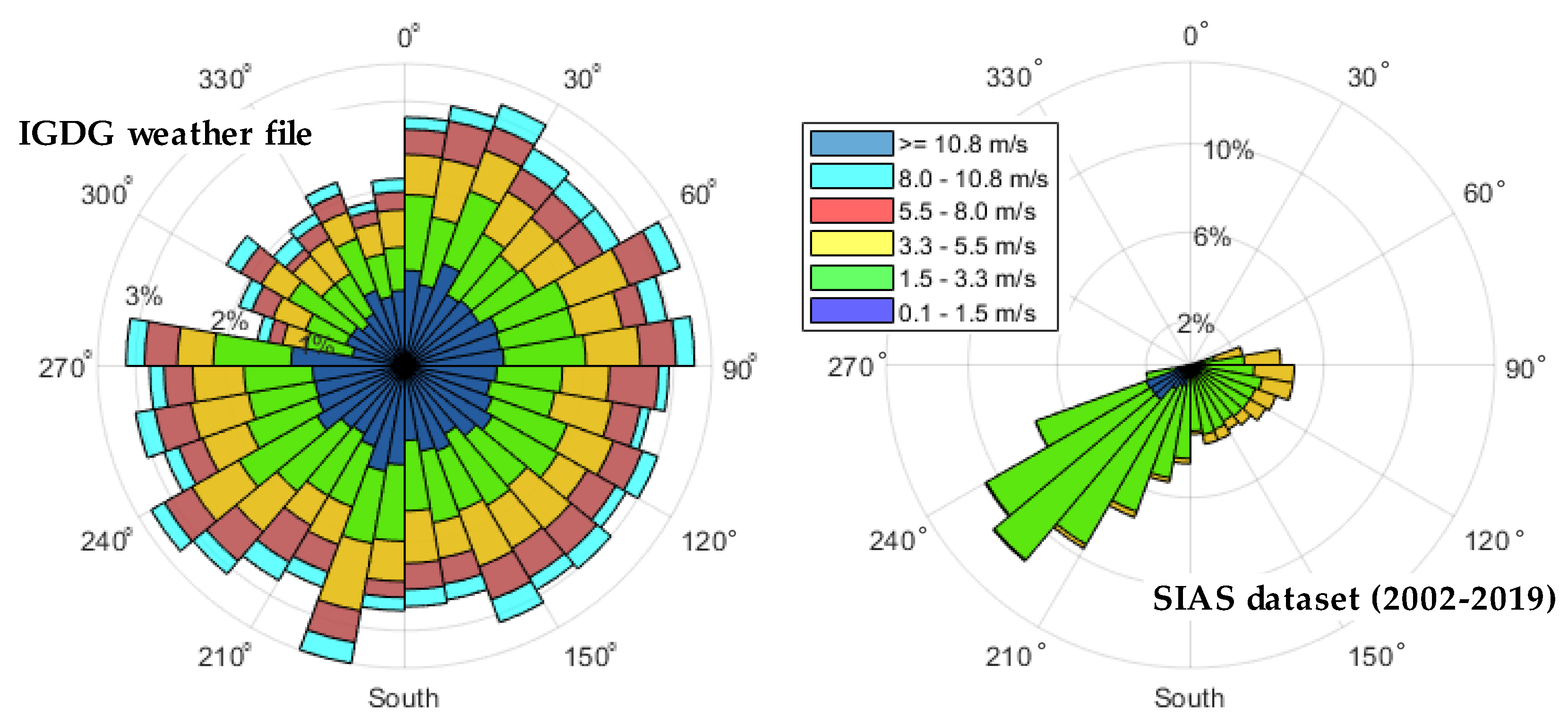
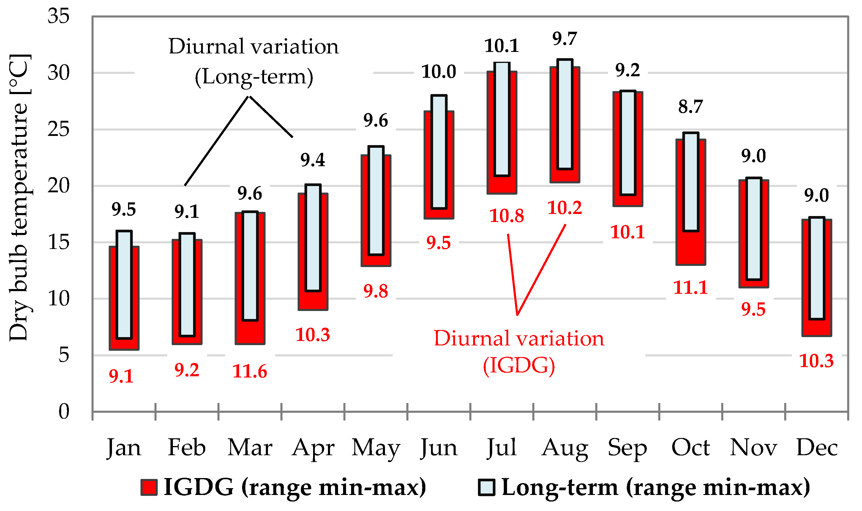
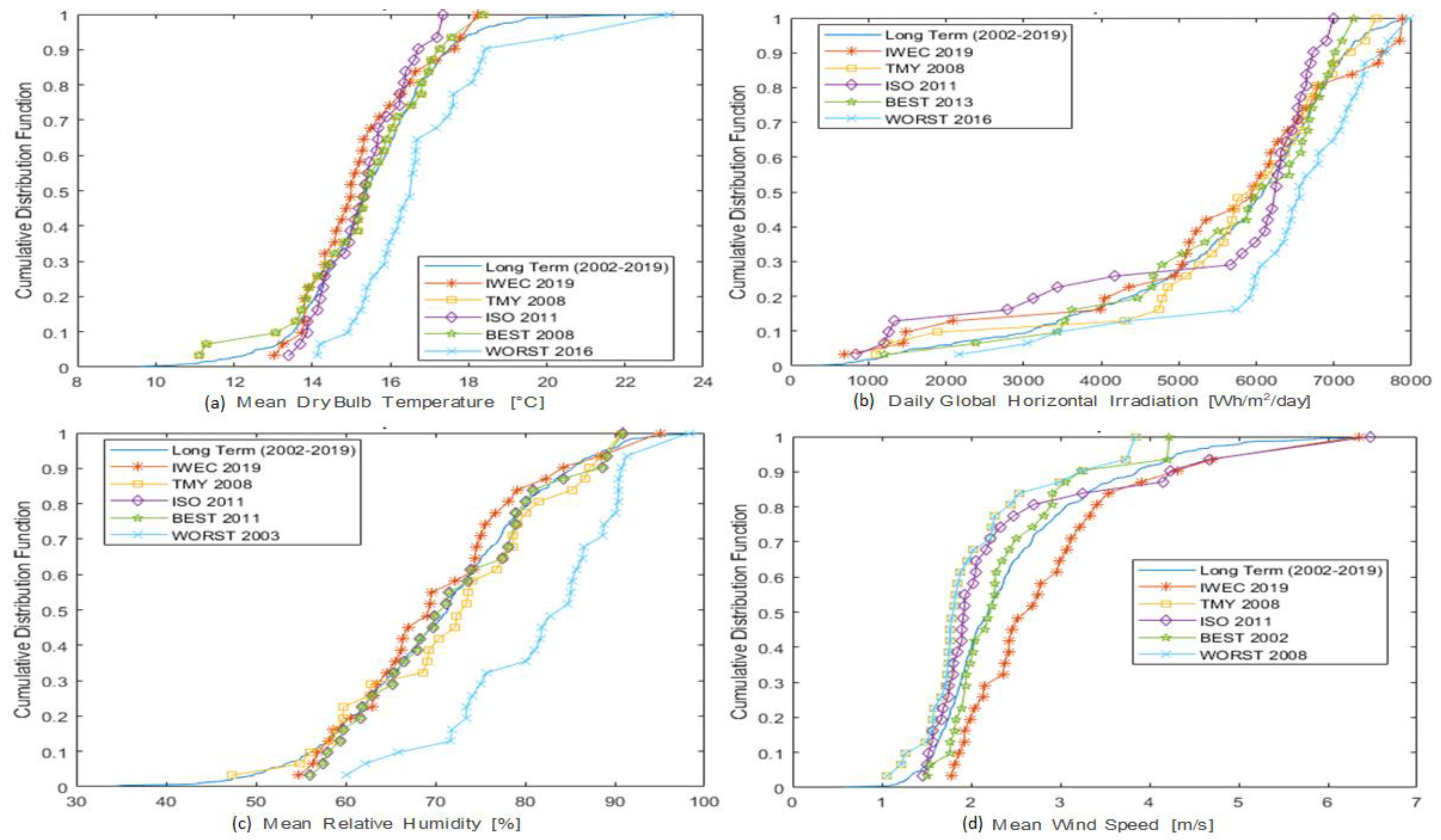
5.1. Statistical Analysis of the SIAS Weather Data

This section discusses the main weather data measured by the SIAS weather station between 2002 and 2019 and compares them with the data included in the weather files available for the airport “Catania Fontanarossa” in the EnergyPlus website (IGDG) and in the website of the Italian Thermotechnical Committee (CTI).

The parameters considered for this analysis are the air temperature, the daily global irradiation on the horizontal plane (GHI), the relative humidity, and the wind speed. The calculation of the daily GHI has implied the integration of the hourly values registered by the pyranometers over every day of the recording period. The analysis was performed after the filling and quality check procedure described in Section 4.

The plots reported in Figure 6 show, for each of the above parameters, the monthly average calculated for the IGDG and the CTI (marker points) along with their range of variation (min, max and mean, solid and dotted lines) for the single years of measurement from 2002 to 2019.

Starting from the dry bulb air temperature (Figure 6a), for each calendar month the mean monthly values referring to the 18 years included in the SIAS dataset can vary within a range whose amplitude is around 3 °C. The IGDG series reports systematically lower mean values, which in some cases fall below the range of variation for the SIAS dataset. This means that a slight increase in the mean air temperature has been observed in the 30 years elapsed from the recording of the IGDG data to the recording of the SIAS weather station. As an example, in July the average of the IGDG series is 24.8 °C, but it rises to 26.1 °C in the SIAS weather dataset. Coherently, a non-negligible overestimation in the mean relative humidity emerges when using the IGDG dataset, especially in the summer months, amounting to around 5% or 10% (Figure 6b).

The GHI shows even more evident differences (Figure 6c). Indeed, the GHI measured by the SIAS weather station is constantly well above the values reported in the IGDG weather file: As an example, in April the mean value is around 4700 Wh/m² in the IGDG dataset, but it rises to 5600 Wh/m² in the SIAS dataset (2002–2019), meaning an increase by 20% on average. In July, the average increases from 6300 Wh/m² in the IGDG dataset to 7300 Wh/m² in the SIAS dataset, which corresponds to 17% higher solar energy available on average.

Finally, the mean wind speed measured by the SIAS weather station is significantly below the values proposed in the IGDG typical year, especially in January and April, despite the fact that the distance between the two weather stations amounts to just a few kilometers (Figure 6d). This difference could originate from a variation in the local wind pattern in the last fifty years, but it is much more likely that the wind speed measured by the SIAS station is affected by the proximity of an industrial district with low-rise warehouses at a distance of approximately 300 m, which can be observed in Figure 3.

As far as the CTI data are concerned, these are generally quite close to the mean SIAS values: Indeed, they derive from a recent (although shorter) recording period and also from the same weather station. The only relevant difference concerns the wind speed (Figure 6d): However, it is important to observe that the wind data included in the CTI weather file refer to a height of 2 m above ground, while all other wind data have been measured at 10 m above ground. This is in the authors’ opinion a serious flaw in the CTI dataset, which implies the need to perform arbitrary conversions through suitable equations in order to make comparisons—and simulations—possible.

One more comparison that is here proposed concerns the wind direction. Figure 7 shows the wind rose plotted both for the IGDG and the entire SIAS dataset: In this case, the wind rose refers to the whole period of 18 years, but similar plots can be obtained if one considers every single year. The wind roses suggest that very different wind patterns emerge from the two data sources. In particular, the prevailing wind direction in the SIAS dataset is from South-West, which is coherent with the presence of Mount Etna in the North-West quadrant, acting as a shield. On the contrary, the wind rose for the IGDG dataset suggests an even distribution for the wind direction, with a slightly lower frequency from North-West. As already discussed for the wind speed, such a significant difference is actually difficult to justify.

Finally, Figure 8 compares, on a monthly basis, the mean values of the daily minimum and maximum dry bulb temperature, and consequently the mean diurnal temperature fluctuation. These data are particularly relevant to calculate the peak daily energy demand and, especially in the summer, to assess the effectiveness of natural ventilation strategies. Now, the long-term measured data show—apart for two months—a non-negligible reduction in the amplitude of the average diurnal temperature variation: As an example, in July this decreases from 10.8 to 10.1 °C. Together with the higher daily minimum temperatures appearing in the SIAS dataset, this is likely to affect the cooling potential of nighttime natural ventilation strategies, which is then over-estimated by the use of the outdated IGDG weather file.

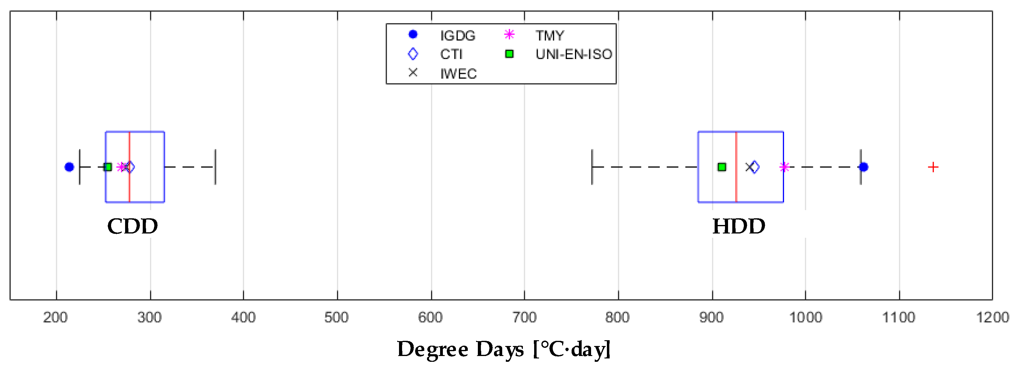
5.2. Selection of the Typical Months and Their Comparison

This section aims at showing that the application of the different procedures outlined in Section 3.1 may lead to the selection of different typical calendar months, hence giving rise to a variety of typical years including different weather data. In fact,

Table 6. Selection of the typical months according to the different procedures.

Method	Jan	Feb	Mar	Apr	May	Jun	Jul	Aug	Sept	Oct	Nov	Dec
IWEC	2011	2006	2012	2019	2005	2009	2005	2007	2013	2015	2019	2008
TMY	2011	2006	2012	2008	2016	2009	2008	2004	2004	2009	2004	2008
ISO	2014	2006	2011	2011	2016	2009	2004	2010	2013	2015	2010	2008

suggests that for only three calendar months (February, June, and December) the three procedures lead to the identification of the same typical month (occurring in 2006, 2009, and 2008, respectively). In five cases, at least one procedure identifies a typical month that does not correspond to the one selected by the other procedures; finally, four calendar months are common for every procedure.

Now, according to the selection procedure discussed in Section 3.1, the resulting typical month takes into account the distances from the long-term cumulative distribution function of each parameter, depending on the weighing factors, and therefore it may differ from the “best” month, i.e., the one with the shortest distance from CDF, associated to each individual parameter. This can be clearly observed in Figure 9, which refers to April and compares—for the main weather parameters—the cumulative distribution functions pertaining to the typical months selected through the various procedures, as well as the best and the worst month (the latter is the month with the longest distance from the long-term cumulative distribution function).

As an example, the typical month selected by the ISO procedure (April 2011) corresponds to the best month in relation to the relative humidity (Figure 9c); however, it is quite distant from the long-term cumulative distribution function with regard to the GHI (Figure 9b). However, all the selected typical months match very well with the long-term cumulative distribution function for temperature (Figure 9a), and this reflects the different weights attributed to the weather parameters by the various procedures.

In order to further highlight this issue,

Table 7. Mean discrepancy between the typical years and the long-term average values for the measured weather parameters.

Variable	Error	IWEC	TMY	ISO
Dry Bulb Temperature [°C]	MBE	−0.08	−0.34	−0.05
	MAE	0.25	0.40	0.32
	RMSE	0.31	0.55	0.42
Relative Humidity [%]	MBE	−0.90	1.03	0.34
	MAE	2.49	2.21	1.43
	RMSE	3.03	2.74	1.69
Wind Speed [m/s]	MBE	0.02	−0.11	0.01
	MAE	0.22	0.19	0.14
	RMSE	0.26	0.23	0.15
Daily Global Solar Irradiation [kWh/m2/day]	MBE	−9.4	23.6	−53.3
	MAE	80.4	69.6	112.6
	RMSE	92.7	88.0	139.4

shows—for the four main weather variables—the values of the Mean Bias Error (MBE), the Mean Absolute Error (MAE), and the Root-Mean-Square Error (RMSE), defined as in the following equations:

$$\mathrm{MBE}=\frac{{\displaystyle {\sum }_{\mathrm{i}=1}^{12}\left({\mathrm{p}}_{\mathrm{i}}-{\mathrm{p}}_{\mathrm{L},\mathrm{i}}\right)}}{12}$$

(10)

$$\mathrm{MAE}=\frac{{\displaystyle {\sum }_{\mathrm{i}=1}^{12}\left|{\mathrm{p}}_{\mathrm{i}}-{\mathrm{p}}_{\mathrm{L},\mathrm{i}}\right|}}{12}$$

(11)

$$\mathrm{RMSE}=\sqrt{\frac{{\displaystyle {\sum }_{\mathrm{i}=1}^{12}{\left({\mathrm{p}}_{\mathrm{i}}-{\mathrm{p}}_{\mathrm{L},\mathrm{i}}\right)}^2}}{12}}$$

(12)

Here, for each calendar month (i), p is the average of the hourly values belonging to the selected typical month, and p_L is the long-term mean value from 2002 to 2019, that is to say:

$${\mathrm{p}}_{\mathrm{L}}=\frac{{\displaystyle {\sum }_{\mathrm{j}=2002}^{2019}\left({\mathrm{p}}_{\mathrm{j}}\right)}}{18}$$

(13)

The results reported in Table 7 basically confirm the outcomes discussed above, but they refer to the entire typical years and not only to a single month as in Figure 9. Compared with the long-term distribution, the ISO procedure allows creating a typical weather year with the lowest RMSE for the relative humidity and wind speed, but with the highest discrepancy in relation to GHI, the latter being almost 50% higher than for the IWEC and TMY typical years (i.e., 139.4 kWh/m²/day versus around 90 kWh/m²/day). The discrepancy of the IWEC and TMY typical years is very similar, even if the IWEC shows a better match with the long-term dry bulb temperature, due to the very high weight attributed to this weather parameter (overall 40% as shown in Table 2).

Further processing included the calculation, for all the recording years, of the Heating Degree Days (HDD) and the Cooling Degree Days (CDD). The HDD—relative to a base outdoor temperature of 18 °C—are integrated from mid-October to mid-April, while the CDD—relative to a base outdoor temperature of 24 °C—are calculated from mid-April to mid-October. Figure 10 compares the values obtained for the IGDG and the CTI typical years against the statistical distribution of the yearly values referring to the SIAS database (whose median value is indicated by the red straight line inside the boxes). As it is possible to observe, the HDD for the IGDG weather file exceeds the maximum value of the SIAS distribution, if one excludes the only outlier that corresponds to an exceptionally cold year (2005). In particular, the HDD for the IGDG file exceeds by 14% the median of the SIAS distribution. Likewise, the CDD for the IGDG weather file is below any other value occurring in the SIAS series, and the difference with the median is around 40%. The HDD and CDD values for the IWEC typical year are very close to the long-term median, while the ISO and the TMY typical years approach respectively the first quartile of the CDD and the third quartile of the HDD, thus suggesting once again that the IWEC is the selection procedure resulting in the most reliable estimation of the average long-term dry bulb temperatures for this site.

5.3. Results of the Dynamic Simulations

As an example of the preparation process needed to organize the weather data in the .epw format. Figure 11 reports—for three consecutive days extracted from the TMY typical year—the trend of dry bulb air temperature, dew point temperature, and Cloud Cover (panel a), with the related sky emissivity and infrared sky irradiance (panel b). When looking at these graphs, it emerges that the sky emissivity is highly influenced by the dew point temperature and the cloud cover, with a peak value of around 0.9 for T_DP = 23 °C and a cloud cover of five tenths. However, sky emissivity values range between 0.82 and 0.90 during the selected days: This affects the infrared irradiance, whose fluctuations between a minimum of about 340 W/m² and a maximum of around 440 W/m² mostly depend on the dry bulb air temperature swinging between 18 and 32 °C.

Moreover, Figure 11c shows how the Global Horizontal Solar Irradiance (solid orange line) is split into the diffuse (solid blue line) and the direct normal (black dashed line) components. Here, it is easy to appreciate the predominance of the direct normal component in the specific climate conditions of Catania, and the influence of the cloud cover (the minimum peak direct component is achieved in the first day when CC is equal to only five tenths). It is also important to consider that the direct normal component refers to a plane normal to the sun ray: For this reason, at sunrise and sunset it can even exceed the global irradiance measured on the horizontal plane.

Before commenting on the differences in the predicted energy needs generated by the different weather datasets, it is worth highlighting a significant methodological difference in the estimation of the solar irradiance components. In fact, while the weather files developed in this research rely on hourly measured values for GHI—split into their diffuse and direct normal components as per the Boland and Ridley model [64]—the IGDG dataset reports hourly derived solar irradiance components obtained through the application of the Erbs’ and the modified Liu-Jordan models to daily (not hourly) integral GHI measurements [11]. Along with the different observation period, this aspect contributes to the big variations reported in

Table 8. Heating and cooling energy needs according to the different weather datasets.

Case	Energy Use	IGDG	TMY	IWEC	ISO
Current Building	Heating [kWh]	4128	2175	2125	2047
	(% difference)	-	−47%	−48%	−50%
	Cooling [kWh]	1885	3095	3143	3072
	(% difference)	-	+64%	+67%	+63%
Insulated Building	Heating [kWh]	2910	1293	1259	1195
	(% difference)	-	−56%	−57%	−59%
	Cooling [kWh]	1675	2698	2748	2670
	(% difference)	-	+61%	+64%	+59%

.

Here, it is possible to observe that significant differences occur in both heating and cooling energy needs predicted through the IGDG (base case) in comparison with the other datasets: The heating energy needs are indeed halved when the simulations are run with one of the developed weather files whereas the cooling needs dramatically increase by about 67% when shifting from the IGDG to the IWEC weather file. In the simulations with the insulated envelope, the relative difference in the heating energy needs predicted by a new weather file and by the old IGDG one is in the ranges from −59% (ISO dataset) to −56% (TMY dataset), while the difference in the cooling energy needs ranges from +59% (ISO weather file) to +64% (IWEC weather file).

This discrepancy is high if compared with the outcomes of previous papers. As an example, Radhi found out that using a typical year based on weather data from 1961 to 1990 underestimates the electricity consumption in the cooling system by up to 14.5% for two buildings in Bahrain, compared with the adoption of recent weather data (from 1992 to 2005) [74]. Koci et al. reported a warming trend in the recent weather of Prague, Czech Republic; consequently, the simulated energy demand for a residential building decreased by 4% to 15% when using recent weather data (2013–2017) instead of historical weather data (1990–2015). The remarkable discrepancy emerging in the present paper can then be attributed not only to the increasing trend in the dry bulb temperature, but also to the high difference observed in the global horizontal irradiation and the wind speed already discussed in Section 5.1, and to the older observation period (1951–1970).

On the contrary, it is possible to state that the choice of a specific selection procedure for the typical year has a minor role, leading to a fluctuation by around 3% or 4% in the results: This is almost negligible if compared with the great inaccuracy deriving from the use of the outdated IGDG weather file.

No simulations using the CTI weather dataset have been run because, as discussed in Section 2, the observation period for this dataset is too short and covers only a sub-period of that used for developing the updated TWYs. Furthermore, several parameters that are necessary to build the weather file, such as wind direction and cloud cover, are missing in the CTI dataset: Accordingly, they should be retrieved from other sources and checked for consistency. Finally, as reported in Section 5.1, the CTI weather dataset reports the wind speed at 2 m above ground, while this is commonly measured at a height of 10 m: A conversion would then be required.

6. Conclusions

This paper has investigated the application of various procedures to the generation of Typical Weather Years representative of recent climate trends in the moderately hot and humid city of Catania (Italy). Weather data recorded from 2002 to 2019 through a stationary meteorological station owned by the Sicilian Agrometeorological Information System (SIAS) and located outside the city context have been compared to two currently available datasets: The one provided by the Italian Thermotechnical Committee (CTI), based on the data coming from the same meteorological station but limited to the period 2002–2009, and the one included in the Italian climatic data collection “Gianni De Giorgio” (IGDG) based on data measured by a different station located in the airport at a distance of just 3 km. The latter relies on outdated data (1951–1970) but is still largely in use for building simulation purposes.

The statistical analysis revealed that the recent weather data show higher values of dry bulb air temperature, lower values of relative humidity (in the range of 5% to 10%), and higher global horizontal irradiance (GHI) than in the old IGDG dataset. Furthermore, the variability in the GHI is more marked in the SIAS dataset because the hourly values included in the IGDG series are not measured but rather derived through a mathematical model starting from daily integral values. This change in the average measured weather data can be due both to a difference in the local conditions and to the global climate variation in the last decades; in any case, it remarkably affects the outcomes of building energy simulations. In fact, the predicted heating energy needs for a poorly insulated typical residential building are halved when the simulations take into account the most recent weather dataset, whereas the cooling energy needs can increase by about 65%. Similar figures recur in the case of insulated envelope, while negligible variance (below 5%) emerges when adopting the other typical years considered in this analysis.

The results of the paper are particularly relevant because they cast light on the urgent need of updating the IGDG weather dataset, which is still widely used by researchers and practitioners in the field of building energy simulation and, at least in the case of Catania, gives rise to inacceptable inaccuracy in the calculation of the energy demand for space heating and cooling. This is the first study concerning this issue and referring to the Mediterranean climate of Southern Italy.

Future work will focus on appraising the effects of using updated weather datasets on a wider set of building typologies through detailed energy simulations, while also investigating the importance of multi-year simulations.

References

1. IEA. 2018 Global Status Report. Available online: https://www.iea.org/reports/2018-global-status-report (accessed on 7 April 2020).
2. Fichera, A.; Frasca, M.; Palermo, V.; Volpe, R. An optimization tool for the assessment of urban energy scenarios. Energy 2018, 156, 418–429. [Google Scholar] [CrossRef]
3. De Wilde, P. Building Performance Analysis, 1st ed.; Wiley Blackwell: Oxford, UK, 2018. [Google Scholar]
4. Hensen, J.L.M.; Lamberts, R. Building Performance Simulation for Design and Operation, 1st ed.; Taylor & Francis: Abingdon, UK, 2011. [Google Scholar]
5. De Masi, R.F.; Gigante, A.; Ruggiero, S.; Vanoli, G.P. The impact of weather data sources on building energy retrofit design: Case study in heating-dominated climate of Italian backcountry. J. Build. Perform. Simul. 2020, 13, 264–284. [Google Scholar] [CrossRef]
6. Cui, Y.; Yan, D.; Hong, T.; Xiao, C.; Luo, X.; Zhang, Q. Comparison of typical year and multiyear building simulations using a 55-year actual weather data set from China. Appl. Energy 2017, 197, 890–904. [Google Scholar] [CrossRef] [Green Version]
7. Wang, L.; Mathew, P.; Pang, X. Uncertainties in energy consumption introduced by building operations and weather for a medium-size office building. Energy Build. 2012, 53, 152–158. [Google Scholar] [CrossRef] [Green Version]
8. Erba, S.; Causone, F.; Armani, R. The effect of weather datasets on building energy simulation outputs. Energy Procedia 2017, 134, 545–554. [Google Scholar] [CrossRef]
9. Pernigotto, G.; Prada, A.; Cóstola, D.; Gasparella, A.; Hensen, J.L.M. Multi-year and reference year weather data for building energy labelling in north Italy climates. Energy Build. 2014, 72, 62–72. [Google Scholar] [CrossRef] [Green Version]
10. Lou, S.; Li, D.H.W.; Huang, Y.; Zhou, X.; Xia, D.; Zhao, Y. Change of climate data over 37 years in Hong Kong and the implications on the simulation-based building energy evaluations. Energy Build. 2020, 222, 110062. [Google Scholar] [CrossRef]
11. IGDG Weather Dataset. Available online: https://energyplus.net/sites/all/modules/custom/weather/weather_files/italia_dati_climatici_g_de_giorgio.pdf (accessed on 7 April 2020).
12. CTI Energia Ambiente (Comitato Termotecnico Italiano). Available online: https://try.cti2000.it (accessed on 7 April 2020).
13. Hall, I.J.; Prairie, R.; Anderson, H.; Boes, E. Generation of a Typical Meteorological Year for 26 SOLMET Stations; Technical Report SAND-78-1601; Sandia National Laboratories: Albuquerque, NM, USA, 1978.
14. Marion, W.; Urban, K. User’s Manual for TMY2; National Renewable Energy Laboratory: Golden, CO, USA, 1995. Available online: http://rredc.nrel.gov/solar/pubs/tmy2 (accessed on 7 April 2020).
15. Wilcox, S.; Marion, W. User’s Manual for TMY3 Data Sets; Technical Report NREL/TP-581-43156; National Renewable Energy Laboratory: Golden, CO, USA, 2008.
16. Thevenard, D.J.; Brunger, A.P. The development of typical weather years for international locations: Part I, algorithms. ASHRAE Trans. 2002, 108, 376. [Google Scholar]
17. Huang, Y.J.; Su, F.; Sheo, D.; Krarti, M. Development of 3012 IWEC2 weather files for international locations (RP-1477). ASHRAE Trans. 2014, 120, 340–355. [Google Scholar]
18. Hygrothermal performance of buildings—Calculation and presentation of climatic data—Part 4: Hourly data for assessing the annual energy for heating and cooling. In ISO 15927-4:2005; ISO: Vernier, Switzerland, 2005.
19. Festa, R.; Ratto, C.F. Proposal of a numerical procedure to select Reference Years. Sol. Energy 1993, 50, 9–17. [Google Scholar] [CrossRef]
20. Lund, H.; Eidorff, S. Selection Methods for Production of Test Reference Years, Appendix D, Contract 284-77 ES DK; Final Report, EUR 7306 EN; Technical University of Denmark: Lyngby, DK, 1980. [Google Scholar]
21. Canadian Weather Energy and Engineering Data Sets (CWEEDS files) and Canadian Weather for Energy Calculations (CWEC files) Updated User’s Manual; Environment Canada and National Research Council of Canada: Ottawa, ON, Canada, 2008.
22. ASHRAE Handbook Fundamentals, S.I. ed.; Chapter 24; American Society of Heating, Refrigerating and Air-Conditioning Systems: Atlanta, GA, USA, 1989.
23. Argiriou, A.; Lykoudis, S.; Kontoyiannidis, S.; Balaras, C.A.; Asimakopoulos, D.; Petrakis, M.; Kassomenos, P. Comparison of methodologies for TMY generation using 20 years data for Athens, Greece. Solar Energy 1999, 66, 33–45. [Google Scholar] [CrossRef]
24. Chan, A.L.S.; Chow, T.T.; Fong, S.K.F.; Lin, J.Z. Generation of a typical meteorological year for Hong Kong. Energy Convers. Manag. 2006, 47, 87–96. [Google Scholar] [CrossRef]
25. Chan, A.L.S. Generation of typical meteorological years using genetic algorithm for different energy systems. Renew. Energy 2016, 90, 1–13. [Google Scholar] [CrossRef]
26. Siu, C.Y.; Liao, Z. Is building energy simulation based on TMY representative: A comparative simulation study on doe reference buildings in Toronto with typical year and historical year type weather files. Energy Build. 2020, 211, 109760. [Google Scholar] [CrossRef]
27. Bre, F.; Fachinotti, V.G. Generation of typical meteorological years for the Argentine Littoral Region. Energy Build. 2016, 219, 432–444. [Google Scholar] [CrossRef]
28. Jiang, Y. Generation of typical meteorological year for different climates of China. Energy 2010, 35, 1946–1953. [Google Scholar] [CrossRef]
29. Kalamees, T.; Jylhä, K.; Tietäväinen, H.; Jokisalo, J.; Ilomets, S.; Hyvönen, R.; Sakub, S. Development of weighting factors for climate variables for selecting the energy reference year according to the EN ISO 15927-4 standard. Energy Build. 2012, 47, 53–60. [Google Scholar] [CrossRef]
30. Kalogirou, S.A. Generation of typical meteorological year (TMY-2) for Nicosia, Cyprus. Renew. Energy 2003, 28, 2317–2334. [Google Scholar] [CrossRef]
31. Kulesza, K. Comparison of typical meteorological year and multi-year time series of solar conditions for Belsk, central Poland. Renew. Energy 2017, 113, 1135–1140. [Google Scholar] [CrossRef]
32. Lee, K.; Yoo, H.; Levermore, G.J. Generation of typical weather data using the ISO Test Reference Year (TRY) method for major cities of South Korea. Build. Environ. 2010, 45, 956–963. [Google Scholar] [CrossRef]
33. Levermore, G.J.; Parkinson, J.B. Analyses and algorithms for new Test Reference Years and Design Summer Years for the UK. Build. Serv. Eng. Res. Technol. 2006, 27, 311–325. [Google Scholar] [CrossRef]
34. Oko, C.O.C.; Ogoloma, O.B. Generation of a Typical Meteorological Year for Port Harcourt zone. J. Eng. Sci. Technol. 2001, 6, 204–214. [Google Scholar]
35. Skeiker, K. Comparison of methodologies for TMY generation using 10 years data for Damascus, Syria. Energy Convers. Manag. 2007, 48, 2090–2102. [Google Scholar] [CrossRef]
36. Yilmaz, S.; Ekmekci, I. The generation of Typical Meteorological Year and climatic database of Turkey for the energy analysis of buildings. J. Environ. Sci. Eng. A 2017, 6, 370–376. [Google Scholar]
37. Bhandari, M.; Shrestha, S.J. Evaluation of weather datasets for building energy simulation. Energy Build. 2012, 49, 109–118. [Google Scholar] [CrossRef]
38. Hosseini, M.; Lee, B.; Vakilinia, S. Energy performance of cool roofs under the impact of actual weather data. Energy Build. 2017, 145, 284–292. [Google Scholar] [CrossRef]
39. Crawley, D.; Lawrie, L. Should we be using just ‘Typical’ weather data in building performance simulation? In Proceedings of the Building Simulation International Conference, Rome, Italy, 2–4 September 2019. [Google Scholar]
40. Rahman, I.A.; Dewsbury, J. Selection of typical weather data (test reference years) for Subang, Malaysia. Building Environ. 2007, 42, 3636–3641. [Google Scholar] [CrossRef]
41. Sawaqed, N.M.; Zurigat, Y.H.; Al-Hinai, H. A step-by-step application of Sandia method in developing typical meteorological years for different locations in Oman. Int. J. Energy Res. 2005, 29, 723–737. [Google Scholar] [CrossRef]
42. Ebrahimpour, A.; Maerefat, M. A method for generation of typical meteorological year. Energy Convers. Manag. 2010, 51, 410–417. [Google Scholar] [CrossRef]
43. Janjai, S.; Deeyai, P. Comparison of methods for generating typical meteorological year using meteorological data from a tropical environment. Appl. Energy 2009, 86, 528–537. [Google Scholar] [CrossRef]
44. Lhendup, T.; Lhendup, S. Comparison of methodologies for generating a typical meteorological year (TMY). Energy Sustain. Dev. 2007, 11, 5–10. [Google Scholar] [CrossRef]
45. Ohunakin, O.S.; Adaramola, M.; Oyewola, O.M.; Fagbenle, R.O. Generation of a typical meteorological year for north-east, Nigeria. Appl. Energy 2013, 112, 152–159. [Google Scholar] [CrossRef]
46. Zang, H.; Wang, M.; Huang, J.; Wei, Z.; Sun, G. A hybrid method for generation of Typical Meteorological Years for different climates of China. Energies 2016, 9, 1094. [Google Scholar] [CrossRef] [Green Version]
47. Pernigotto, G.; Prada, A.; Cappelletti, F.; Gasparella, A. Impact of reference years on the outcome of multi-objective optimization for building energy refurbishment. Energies 2017, 10, 1925. [Google Scholar] [CrossRef] [Green Version]
48. Pernigotto, G.; Prada, A.; Gasparella, A.; Hensen, J.L.M. Analysis and improvement of the representativeness of EN ISO 15927-4 reference years for building energy simulation. J. Build. Perform. Simul. 2014, 7, 391–410. [Google Scholar] [CrossRef] [Green Version]
49. Sorrentino, G.; Scaccianoce, G.; Morale, M.; Franzitta, V. The importance of reliable climatic data in the energy evaluation. Energy 2012, 48, 74–79. [Google Scholar] [CrossRef]
50. Kim, S.; Zirkelbach, D.; Künzel, H.M.; Lee, J.-H.; Choi, J. Development of test reference year using ISO 15927-4 and the influence of climatic parameters on building energy performance. Build. Environ. 2017, 114, 374–386. [Google Scholar] [CrossRef]
51. David, M.; Adelard, L.; Lauret, P.; Garde, F. A method to generate Typical Meteorological Years from raw hourly climatic databases. Build. Environ. 2010, 45, 1722–1732. [Google Scholar] [CrossRef]
52. Yang, L.; Lam, J.C.; Liu, J. Analysis of typical meteorological years in different climates of China. Energy Convers. Manag. 2007, 48, 654–668. [Google Scholar] [CrossRef]
53. Ohunakin, O.S.; Adaramola, M.S.; Oyewola, O.M.; Fagbenle, R.L.; Abam, F.I. A Typical Meteorological Year Generation Based on NASA Satellite Imagery (GEOS-I) for Sokoto, Nigeria. Int. J. Photoenergy 2014, 2014, 468562. [Google Scholar] [CrossRef] [Green Version]
54. Arima, Y.; Ooka, R.; Kikumoto, H. Proposal of typical and design weather year for building energy simulation. Energy Build. 2017, 139, 517–524. [Google Scholar] [CrossRef]
55. Bevilacqua, P.; Bruno, R.; Arcuri, N. Green roofs in a Mediterranean climate: Energy performances based on in-situ experimental data. Renew. Energy 2020, 152, 1414–1430. [Google Scholar] [CrossRef]
56. Chiesa, G.; Grosso, M. The influence of different hourly typical meteorological years on dynamic simulation of buildings. Energy Procedia 2015, 78, 2560–2565. [Google Scholar] [CrossRef] [Green Version]
57. Lupato, G.; Manzan, M. Italian TRYs: New weather data impact on building energy simulations. Energy Build. 2019, 185, 287–303. [Google Scholar] [CrossRef]
58. Kočí, J.; Kočí, V.; Maděra, J.; Černý, R. Effect of applied weather data sets in simulation of building energy demands: Comparison of design years with recent weather data. Renew. Sustain. Energy Rev. 2019, 100, 22–32. [Google Scholar] [CrossRef]
59. Vasaturo, R.; van Hooff, T.; Kalkman, I.; Blocken, B.; van Wesemael, P. Impact of passive climate adaptation measures and building orientation on the energy demand of a detached lightweight semi-portable building. Build. Simul. 2018, 11, 1163–1177. [Google Scholar] [CrossRef] [Green Version]
60. Finkelstein, J.M.; Schafer, R.E. Improved goodness-of-fit tests. Biometrika 1971, 58, 641–645. [Google Scholar] [CrossRef]
61. US Department of Energy. EnergyPlus Version 8.9. Available online: https://energyplus.net/documentation (accessed on 7 April 2020).
62. ASHRAE Handbook Fundamentals, S.I. ed.; Chapter 1: Psychometrics; American Society of Heating, Refrigerating and Air-Conditioning Systems: Atlanta, GA, USA, 2013.
63. Bianchi, C.; Smith, A.D. Localized Actual Meteorological Year File Creator (LAF): A tool for using locally observed weather data in building energy simulations. SoftwareX 2019, 10, 100299. [Google Scholar] [CrossRef]
64. Boland, J.; Ridley, B. Models of Diffuse Solar Fraction. In Modeling Solar Radiation at the Earth’s Surface; Springer: Berlin/Heidelberg, Germany, 2008. [Google Scholar]
65. UNI/TS 10349-1; Riscaldamento e raffrescamento degli edifici—Dati Climatici—Parte 1: Medie Mensili per la Valutazione della Prestazione Termo-Energetica Dell’edificio e Metodi per Ripartire l’Irradianza Solare Nella Frazione Diretta e Diffusa e per Calcolare l’Irradianza Solare su di una Superficie Inclinata; Ente Nazionale di Unificazione: Milan, Italy, 2016. (In Italian)
66. Walton, G.N. Thermal Analysis Research Program Reference Manual; NBSSIR 83-2655; National Bureau of Standards: Washington, DC, USA, 1983; p. 21.
67. Clark, G.; Allen, C. The estimation of atmospheric radiation for clear and cloudy skies. In Proceedings of the 2nd National Passive Solar Conference (AS/ISES), Philadelphia, PA, USA, 16–18 March 1978; pp. 675–678. [Google Scholar]
68. Smith, A.; Lott, N.; Vose, R. The Integrated Surface Database: Recent developments and partnerships. NOAA’s National Climatic Data Center, Asheville, North Carolina. Bull. Am. Meteor. Soc. 2011, 92, 704–708. [Google Scholar] [CrossRef]
69. ASHRAE Handbook—Fundamentals, S.I. ed.; Chapter 26 Ventilation and Infiltration; American Society of Heating, Refrigerating and Air-Conditioning Systems: Atlanta, GA, USA, 2009.
70. UNI/TS 11300-1, Prestazioni Energetiche Degli Edifici—Parte 1: Determinazione del Fabbisogno di Energia Termica dell’Edificio per la Climatizzazione Estiva ed Invernale; Ente Nazionale di Unificazione: Milan, Italy, 2014. (In Italian)
71. EN 15251; Indoor Environmental Input Parameters for Design and Assessment of Energy Performance of Buildings-Addressing Indoor Air Quality, Thermal Environment, Lighting and Acoustics; European Committee for Standardisation: Brussels, Belgium, 2007.
72. Salvati, A.; Palme, M.; Chiesa, G.; Kolokotroni, M. Built form, urban climate and building energy modelling: Case-studies in Rome and Antofagasta. J. Build. Perform. Simul. 2020, 13, 209–225. [Google Scholar] [CrossRef]
73. Santamouris, M. Cooling the cities—A review of reflective and green roof mitigation technologies to fight heat island and improve comfort in urban environments. Sol. Energy 2014, 103, 682–703. [Google Scholar] [CrossRef]
74. Radhi, H.A. Comparison of the accuracy of building energy analysis in Bahrain using data from different weather periods. Renew. Energy 2009, 34, 869–875. [Google Scholar] [CrossRef]
Figure 1. North view of the apartment block (left-hand side) and plan of a typical floor (right-hand side).
Energies 13 04115 g001
Figure 2. Axonometric view of the thermal model with two apartments per floor (pink surfaces: Adiabatic; blue surfaces: Exterior; white surfaces: Shadings).
Energies 13 04115 g002
Figure 3. Position of the weather stations in relation to the city of Catania site.
Energies 13 04115 g003
Figure 4. Picture of the Sicilian Agrometeorological information system (SIAS) weather station and its probes.
Energies 13 04115 g004
Figure 5. Examples of the filling procedure. (a) 0–6 h gaps. (b) 6–24 h gaps, (c) 24–72 h gaps (the dotted lines correspond to the data added through the filling procedure).
Energies 13 04115 g005
Figure 6. Average monthly values for the main weather data. The curves identify the range of variation for the single actual years. (a) Dry bulb temperature; (b) relative humidity; (c) daily global horizontal irradiation; (d) wind speed.
Energies 13 04115 g006
Figure 7. Wind rose for the EnergyPlus website (IGDG) weather file (left-hand side) and for the entire long-term SIAS dataset (right-hand side).
Energies 13 04115 g007
Figure 8. Monthly mean values for the daily minimum and maximum dry bulb temperatures (and corresponding diurnal temperature fluctuations).
Energies 13 04115 g008
Figure 9. Cumulative distribution: Comparison among long-term measurements and selected typical months for April. (a) Dry bulb temperature, (b) daily global horizontal irradiation, (c) relative humidity, (d) wind velocity.
Energies 13 04115 g009
Figure 10. Heating degree days (HDD) and the cooling degree days (CDD): Comparison among typical years and long-term distribution.
Energies 13 04115 g010
Figure 11. Time trend of some weather variables (21–23 August 2019, TMY typical year). (a) Input data to calculate the horizontal infrared sky irradiance; (b) sky emissivity and horizontal infrared sky irradiance; (c) components of the solar irradiance.
Energies 13 04115 g011