Abstract
Optimization of heat transfer systems (HTSs) benefits energy efficiency. However, current optimization studies mainly focus on the improvement of system design, component design, and local process intensification separately, which may miss the optimal results and lack reliability. This work proposes a synergetic optimization method integrating levels of the local process, component to system, which could guarantee the reliability of results. The system-level optimization employs the heat current method and hydraulic analysis, the component level optimization adopts heuristic optimization algorithm, and the process level optimization applies the field synergy principle. The introduction of numerical simulation and iteration provides the self-consistency and credibility of results. Optimization results of a multi-loop heat transfer system present that the proposed method can save 16.3% pumping power consumption comparing to results only considering system and process level optimization. Moreover, the optimal parameters of component originate from the trade-off relation between two competing mechanisms of performance enhancement, i.e., the mass flow rate increase and shape variation. Finally, the proposed method is not limited to heat transfer systems but also applicable to other thermal systems.
1. Introduction
Thermal energy is still of great importance in modern society. A heat transfer system (HTS) is widely used to transport thermal energy, its performance improvement benefits the energy efficiency improvement, and hence efficient and reliable optimization methods and strategies for HTS are necessary [1]. Current related studies can be divided into three levels from top to bottom, i.e., the system parameter level, component design level, and local process intensification level. In the system level, many studies apply various algorithms to optimize the structure and operating parameters such as heat transfer area and operation cost. Ponce-Ortega et al. [2] optimized a heat transfer network including streams with phase change using an mixed integer nonlinear programming MINLP model. Adjiman et al. [3] used the branch and bound method to minimize the total heat transfer area of a heat transfer network. Ravaganani et al. [4] combined the pinch-point analysis and genetic algorithm to minimize the total cost of a heat exchange system. Sameti and Haghighat [5] recently presented a detailed review for optimization researches focusing on district heating and cooling network. On the other hand, there are also contributions of system optimization employing different optimization principles, where entropy generation minimization principle (EGMP) and exergy destruction rate minimization are two most accepted principles [6,7]. Lavric [8] used the EGMP to optimize a cooling system to obtain its optimum topology and working conditions. Ahmadi et al. [9] conducted a multi-objective optimization based on the exergy-based optimization method. Kerdan et al. [10] developed an exergy-based multi-objective optimization tool for non-domestic building system optimization, which could find the optimal retrofit measures by minimizing energy use, exergy destructions, and thermal discomfort. Song et al. [11] proposed an exergy destruction reduction algorithm to optimize mixed refrigerant systems for energy-efficient natural gas liquefication. Marty et al. [12] proposed the optimization of a geothermal plant to balance the distribution between an organic Rankine cycle system and a district heating network connected in parallel based on the exergetic analysis. However, the complexity and coupling relation of HTS increase drastically when the scale of the system increases [13]. Simply stacking governing equations of components only offers a plain model, which is hard for simulation and further optimization. An effective solution for this problem is the heat current method developed by the authors’ group [14], which uses the concept of a re-defined thermal resistance of heat exchangers and reveals the global heat transfer law in HTS. Moreover, combining the heat current model and circuitous philosophy directly gives the governing equations of HTSs without unnecessary intermediate parameters, and hence the optimization can be simplified effectively [15,16,17,18,19].
In the component design level, current studies mainly focus on the optimal design of heat exchangers. Various optimization criteria and principles have been proposed, such as entropy generation rate, exergy destruction rate, performance evaluation criteria (PEC), and lifetime cost analysis (LCA). Ahmadi [20] analyzed a heat exchanger to minimize its entropy generation and total annual cost. Xie et al. [21] applied the EGM on a pin-fin heat exchanger to determine the optimal length of pin-fins. They also used the constructal law to obtain the optimal diameter and shape of pin-fins. Misra et al. [22] employed the exergy destruction minimization method to optimize the thermal performance of an earth-air tunnel HTS. Valencia et al. [23] proposed a multi-objective optimization scheme for the evaporator in an organic Rankine cycle to balance the irreversibility of heat transfer and the investment costs. Li et al. [24] applied the entransy dissipation-based thermal resistance (EDTR) to evaluate serrated fin in plate-fin heat exchangers and found that the results based on EDTR objective functions are better than those based on traditional objective functions. There are also studies not only focus on the optimization design but also account for the reliability of results. Wang et al. [25] combined numerical simulation and optimization algorithms to optimize the heat transfer performance and exergy destruction of slotted fins in heat exchangers, which offers reliable results due to the interaction between numerical simulation and neural network as well as the genetic algorithm. Li et al. [26] proposed a multidisciplinary design optimization method for the cooling turbine blade based on reliability, which could improve the performance of the cooling turbine blade.
Current studies for local heat transfer process optimization mainly focus on modifying the flow field to enhance heat transfer by using different empirical means, where the entropy generation minimization theory [27,28] was also applied. On the other hand, the field synergy principle (FSP) proposed by Guo et al. offers a theoretical analysis framework for the analysis and optimization of convective heat transfer processes [29,30]. A series of convective heat transfer optimization works have been conducted based on the FSP. For instance, Meng et al. [31] developed the alternating elliptical axis tube which could efficiently enhance convective heat transfer in the tube. Chen et al. [32] compared the entropy minimization principle and the entransy dissipation-extreme principle both from optimization theory and results. A recently published review [33] provides more detailed information.
A problem lies in the above works is that all optimizations are performed independently without interaction. In the system level, the optimization is generally performed with empirically estimated parameters such as design geometry, heat transfer coefficients, and pressure drops in the HTS. Overall heat transfer coefficients and pressure drops in the HTS are heavily influenced by operation conditions [34]. Therefore, the estimated values of such parameters can most likely not reflect the actual performance of the HTS. A feasible solution is to numerically simulate local heat transfer processes in HTSs using computational fluid dynamics (CFD) [35] to provide the credibility, and parameters obtained from simulation results can be used as boundary conditions. Moreover, optimization results often deviate from simulation conditions, and hence the simulation is required once more to determine these parameters. For the self-consistency of calculation, an iterating and updating strategy is required.
In this study, a synergetic optimization method for HTSs integrating all three levels of optimization is proposed. A typical HTS is taken as an example and optimized to minimize its pumping power consumption. The system-level optimization combines the heat current method and hydraulic analysis, the component design level optimization uses the heuristic algorithm, and the local heat transfer process optimization is performed numerically based on the FSP. An iterating and updating strategy of system parameters is realized using a multi-disciplinary optimization platform. Finally, optimization results are analyzed to show the advantages of the proposed synergetic method, and the mechanism of optimal parameters is briefly discussed.
2. Physical Model and Optimization Problem of the HTS
A typical multi-loop HTS is investigated in this work to present the proposed optimization method. As Figure 1 presents, the HTS contains a hot water reservoir, an evaporator, two counter-flow heat exchangers, and three variable speed pumps (VSPs). The tubes in the evaporator are elliptical tubes due to their heat transfer enhancement comparing to round tubes [36]. Temperatures of fluids are denoted by 1–3 according to the fluid loop, and subscripts h and c refer to the hot and cold fluid, respectively. The temperatures of hot water in the tank and refrigerant remain as T1,h, and Te, respectively. In the system operation, VSPs drive working fluids, by which the heat duty is transferred from the hot water reservoir to the refrigerant.
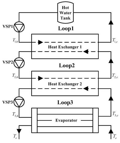
Figure 1.
Sketch of a multi-loop heat transfer system [37].
The design of this HTS could be optimized by choosing design parameters, such as the geometry design of elliptical tubes, heat transfer areas of heat exchangers, and other operating parameters. In this study, the optimization objective is chosen as minimizing the pumping power consumption P under a given heat transfer duty Q. Besides, heat transfer areas of components are given in advance. Decision variables of this optimization problem can be attributed to three levels: (1) operation parameters, i.e., operating frequencies of three VSPs, ωi (i = 1, 2, 3), (2) geometry design parameter, i.e., the semi-minor axis rb of the elliptical tube under a constant semi-major axis ra, and (3) local heat transfer process parameters, i.e., the flow and temperature fields in the elliptical tubes, U(x,y,z) and T(x,y,z).
3. Synergetic Optimization Method
3.1. System Optimization Model
3.1.1. Heat Transfer and Fluid Flow Constraints of the HTS
The heat current model of the HTS shown in Figure 1 is given in Figure 2, where the heat flow direction in the HTS is presented. Applying the Kirchhoff’s Voltage Law (KVL) on the heat current model yields the governing equation.
where Q is the heat transfer rate in the system. R1, R2, and R3 are inlet temperature difference-based thermal resistances of heat exchanger HX1, HX2 and the evaporator, respectively. Their expressions are [14]:
where (i = 1, 2, 3) is the overall heat transfer coefficient of each heat exchanger. In the calculation, these parameters are initialized using estimated values and hence are marked by overline. Their values will be updated using simulation results. Ai stands for the heat transfer area, and Gi stands for the heat capacity rate of working fluids, i.e., the product of mass flow rate and specific heat (mcp)i.
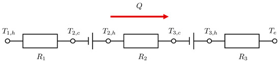
Figure 2.
Heat current model of the heat transfer system (HTS).
The hydraulic constraints of the system are also required, which can be established by the balance relation of driving force and resistance of the fluid flow. The flow resistance in the system comes from fluid pressure drops in heat exchangers and pipelines. The total flow resistance in the i-th loop is
where Hi is the total head, Hs,i is the static head, Hd,i is the dynamic head of the pipeline network, and He,i is the head from pressure drops in heat exchangers. Static heads Hs,i are controlled by the structure of the pipeline network and can be treated as constants, while the dynamic head Hd,i is [19]:
where bi are lumped parameters determined by the pipeline.
where ρi is the density of the working fluid, Si is the sectional area of the pipeline, Li stands for the length of the pipeline, Fi refers to Darcy’s coefficient, di stands for the diameter of the pipeline, and Ki is the local resistance coefficient [37]. Besides, heads related heat exchangers He,i are determined by internal pressure drops:
where and are pressure drops of both hot and cold fluids in heat exchangers. Like the overall heat transfer coefficients, here pressure drops are also initialized by estimated values to start the calculation and to be updated with simulation results.
The governing equation of VSPs is required to determine the driving force of working fluids as follows:
where aj,i (j, i = 0, 1, 2) are characteristic parameters of VSPs, and they remain constants in the optimization procedure. Therefore, the hydraulic constraint equation of the HTS can be obtained:
The optimization objective, in this case, is the total pump power consumption of VSPs, which could be expressed as:
3.1.2. Optimization Equations of the HTS
The Lagrange multiplier method is applied to derive the optimization equations of the problem, and the Lagrange function is constructed as follows:
where α and βi are Lagrange multipliers. Taking partial differentials of the Lagrange function with respect to each variable (mi and ωi) and letting them equal to zero yields the Lagrange equations:
Partial derivatives related to thermal resistances are provided in Appendix A. Solving these Lagrange equations together with heat current Equation (1) as well as the hydraulic constraint Equation (12) gives optimal results. However, the obtained solution is the optimal parameters with estimated overall heat transfer coefficients and pressure drops, and . Therefore, these optimization results are to be updated using fluid flow simulation results.
3.2. Simulation and Optimization of Heat Exchangers
3.2.1. Simulation of Heat Exchangers HX1 and HX2
CFD simulation is used to determine overall heat transfer coefficients ki and pressure drops Δpi,h and Δpi,c under different operating conditions. Heat exchangers 1 and 2 are counter-flow plate exchangers with periodical structures, and hence they can be divided into heat transfer units consisting of two fluid channels and a heat conduction plate between them. Figure 3 presents the sketch and the computational grid of a heat transfer unit of HX1 and HX2. The outlet of each fluid in the computational model is extended to prevent possible backflows and vortexes.
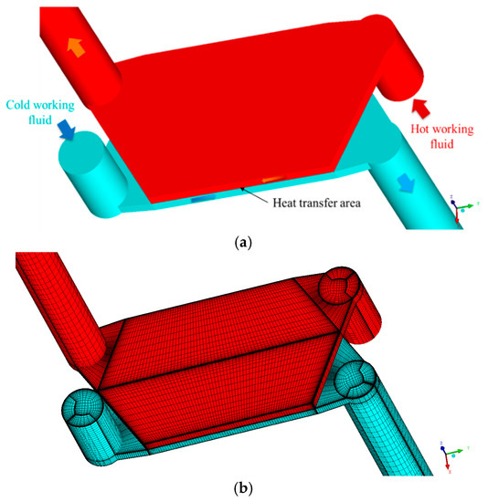
Figure 3.
Heat transfer unit in the heat exchangers 1 and 2: (a) sketch and (b) computation grids.
Boundary conditions for the simulation are given as follows. The entrance of the unit is treated with the velocity-inlet condition, where the velocities are set by mass flow rates mi:
where A1,inlet and A2,inlet are inlet sectional areas of heat transfer units to calculate the average flow velocity. Nu1 and nu2 are numbers of heat transfer units contained in two heat exchangers, respectively. The outlets adopt the standard pressure-outlet condition. The plate in the heat transfer unit is a copper plate with a thickness of 1.5 mm, and no-slip wall condition with conjugate heat conduction is assigned to the plate. Besides, the upper and lower surfaces are assigned to the periodic boundary condition, and the lateral sides and other zones contacted with the environment are treated with insulating surfaces.
The gravity force, thermal radiation, and viscous heat generation are neglected in the simulation. The working fluids in three loops are water, which is regarded as incompressible, and its properties are treated as constant. Therefore, the governing equations are [38]:
where U is the velocity, p stands for the pressure, and λ is the thermal conductivity. The simulation is implemented by ANSYS Fluent, and the Semi-Implicit Method for Pressure Linked Equations-Consistent (SIMPLEC) algorithm is used. The renormalization group (RNG) k-ε model is additionally applied when the flow is turbulent. The overall heat transfer coefficients ki and pressure drops Δpi,h and Δpi,c are extracted from simulation results when the computation reaches convergence. Specifically, the overall heat transfer coefficient is determined employing heat transfer rate qi, the heat transfer area Au,I and logarithm mean temperature difference (LMTD) ΔTlm,I of heat transfer units.
3.2.2. Convective Heat Transfer Optimization in the Evaporator
Both design parameters and convective heat transfer processes in the evaporator are to be optimized. The optimization method of the convective heat transfer process under a certain geometry condition is presented first. The flow in the evaporator remains laminar flow due to the small heat transfer duty Q and mass flow rate m3. The corresponding governing equations for the optimal flow field are [32,33]:
where F is an additional volume force determined by:
where CΦ is a parameter relating to the viscous dissipation rate:
Here, C0, C1, and C2 are Lagrange multipliers introduced, and C0 is a constant [39], while C1 and C2 are field functions of temperature T, velocity U, and spatial coordinates (x, y, z).
Equation (27) is the momentum equation of the working fluid with an additional volume force F. The value of CΦ represents the strength of volume force, and different values of CΦ lead to different longitudinal vortex structures. Equation (28) is the governing equation of Lagrange multiplier C1. Solving Equations (27) and (28) as well as the mass and energy conservation equations offers the optimal fluid velocity field with the largest overall heat transfer coefficient for a laminar forced convection process with a prescribed inlet velocity and a specific viscous dissipation rate [33].
The geometry and boundary conditions used in the evaporator optimization are as follows. The evaporator consists of 15 copper elliptical tubes with a length of 150 mm and a wall thickness of 0.7 mm. The structure sketch of the evaporator is presented in Figure 4. Besides, the semi-major axis of the elliptical tube ra remains 5 mm while the semi-minor axis of the elliptical tube rb varies between 2 mm to 5 mm. Since the length-diameter ratio of the tube is quite large, the elliptical tubes in the evaporator can also be divided into heat transfer units to simplify the numerical calculation. The heat transfer unit here is chosen as a segment of the elliptical tube with a length of 20 mm, and the computation grid for ra = 5 mm and rb = 2.5 mm is shown in Figure 5. The computation grid is the combination of the structured hexahedron grid in the boundary layer and the unstructured hexahedron grid in the inner domain to improve the calculation precision, and the grid number is around 116,000. Comparing with earlier works on the convective heat transfer optimization in tubes [31,32], the grid number is large enough to ensure the grid independency.
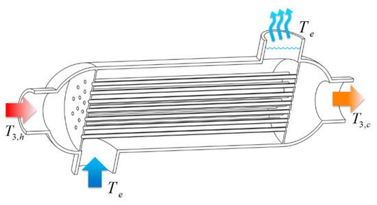
Figure 4.
Sketch of the evaporator.
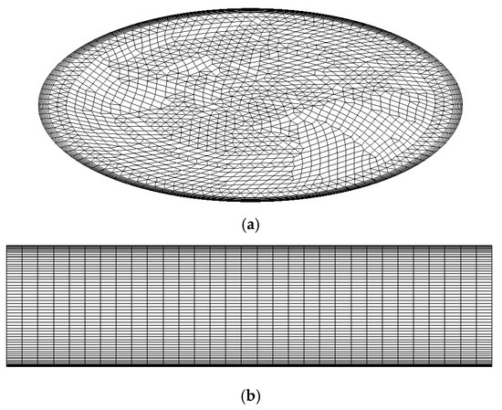
Figure 5.
Grids of a heat transfer unit in an elliptical tube where ra = 5 mm and rb = 2.5 mm: (a) x–y direction and (b) z–y direction.
Boundary conditions for the optimization calculation are as follows. Since the refrigerant evaporates from the liquid to vapor, its temperature keeps at the boiling point Te. Besides, in the evaporator, the thermal resistance of heat conduction in the tube wall can be neglected due to the high conductivity of the tube wall. Therefore, the temperature of the tube wall is regarded as Te. That is, the tube wall adopts the condition of the no-slip wall with a constant temperature. Moreover, periodical conditions are applied to the inlet and outlet of the heat transfer unit. Finally, the mass flow rate in each tube mu can be calculated by the total mass flow rate m3 and the number of tubes in the evaporator nt:
The heat transfer area of the heat transfer unit Au is given as:
where Lu is the length of the heat transfer unit of elliptical tubes (20 mm), D is the perimeter of the tube cross-section, and can be calculated by Ramanujan’s approximation [40]:
The total heat transfer area of the evaporator A3 is then derived as:
where L is the length of the tube (150 mm). The overall heat transfer coefficient of the evaporator, k3, is also determined by the LMTD approach.
The discretization scheme and algorithms in the simulation are as follows: the SIMPLEC algorithm is applied for the coupling of pressure and velocity, the second order upwind scheme is adopted for the momentum and energy conservation equation, and the QUICK (Quadratic Upstream Interpolation for Convective Kinematics) scheme is used for the governing equation of Lagrange multiplier C1. Considering the robustness of the computation, the value of CΦ is chosen to be −4.8, which leads to a 4-vortex structure in the flow field [37,41].
3.3. Synergetic Optimization Procedure
The system-level optimization, heat exchanger simulation, and local heat transfer process level optimization in elliptical tubes of the evaporator have been presented, and they are required to be integrated by a synergetic optimization strategy. Besides, the local heat transfer optimization above is performed. Moreover, with fixed geometry configuration of elliptical tubes, while the design optimization of elliptical tubes is absent.
First, the heat transfer system with a given semi-minor axis of elliptical tubes rb is considered. The system-level optimization of the HTS is first performed with estimated parameters, i.e., estimated overall heat transfer coefficients and estimated pressure drops, and . Next, the CFD simulation is conducted for plate heat exchangers HX1, HX2. The convective heat transfer optimization in the evaporator is also performed using the numerical simulation. Overall heat transfer coefficients ki and pressure drops Δpi,h and Δpi,c derived from computation results generally differ from estimated values, and if deviations between actual parameters and estimated parameters, εi, , and are out of the tolerance range, they will be then updated:
where ϕi, Ψi,h, and Ψi,c are relaxation factors, and they are empirically chosen to be 0.7, 0.5, and 0.5, respectively. After the update, the system optimization will be performed again with updated , , and . This iteration continues until deviations are within the tolerance range. Once the iteration converges, the optimal pump power consumption P with the current semi-minor axis rb can be derived from optimization results.
The last step of the synergetic optimization is to search the optimum semi-minor axis rb within the given range to obtain the minimum pumping power consumption, where the downhill simplex (DS) algorithm is employed. When the iteration process of DS algorithm converges, the minimized pumping power consumption and corresponding optimal operation parameters including the frequencies of VSPs ωi, the semi-minor axis of elliptical tubes rb, and the optimal flow field U in the elliptical tubes are obtained. That is, the optimization of the elliptical tubes includes both component level and local heat transfer process level optimization. The component level optimization is to find the optimal semi-minor axis rb, and the local heat transfer process level optimization is to find the optimal flow field. Figure 6 gives a graphical summary of the proposed synergetic optimization method, and Figure 7 presents a detailed flowchart of the nested iteration process.
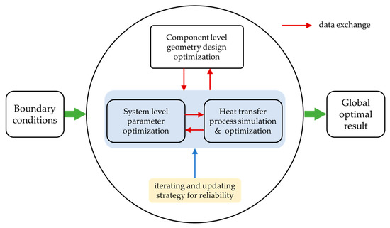
Figure 6.
Sketch of the proposed synergetic optimization method.
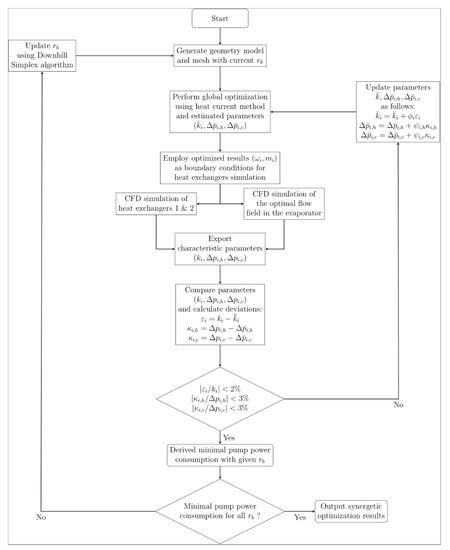
Figure 7.
Flowchart of the synergetic optimization procedure.
4. Optimization Results and Discussion
The main conditions used in the HTS optimization case are presented in Table 1. Besides, the geometry parameters of heat exchangers 1 and 2, characteristic parameters of the pipeline network, and VSPs remain the same in the optimization computation. The characteristic parameters of the pipeline network and VSPs are presented in Table 2 and Table 3, which are identical with them in References [37,42] for comparison.

Table 1.
Conditions used in the HTS optimization.
Table 2.
Characteristic parameters of the pipeline network.
Table 3.
Characteristic parameters of the variable speed pumps (VSPs).
Table 4 compares the results of two cases, i.e., with and without component geometry optimization. Both two cases include system-level optimization and local convective heat transfer process optimization. In the case with component geometry optimization, the Reynolds number of the elliptical tube flow in the evaporator is 425.27, which verifies the working condition of laminar flow. The comparison shows that the optimized pumping power consumption P, decreases from 19.35 to 16.2 W with the semi-minor axis length decreases from 5.0 to 3.75 mm. Besides, the heat transfer area of the evaporator decreases from 0.071 to 0.0623 m2, and the operating frequencies of VSPs and the mass flow rates in loops also decrease. Therefore, the proposed synergetic optimization method combining the local heat transfer process, geometrical design, and system parameter optimization is more efficient for both energy and cost-saving.
Table 4.
Comparison of synergetic optimization results of the HTS.
Figure 8 presents the sectional velocity (Figure 8a) and the temperature field (Figure 8b) of the elliptical tubes after the optimization procedure converges. The results present that the optimal flow field for the elliptical tube has vertical vortexes to enhance the internal convective heat transfer. However, compared to the original flow field, the temperature field does not change significantly, which is attributed to the limited strength of volume force F. Besides, the convective heat transfer in the elliptical tube is indeed enhanced since the velocity field is changed, and the average field synergy angle of the entire field is increased [43].
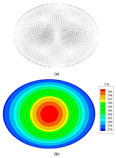
Figure 8.
Optimal flow field in the elliptical tube with rb/ra = 0.75: (a) velocity field on section and (b) temperature distribution on section.
Figure 9 presents the iteration process of searching the optimal semi-minor axis length rb within the given range, and iteration points are not distributed uniformly due to the application of the heuristic algorithm. Each point stands for an optimal total pumping power consumption P under a certain rb, and among them, the minimal total pump consumption point is the optimal one considering the geometry design optimization. The results read that the optimal semi-minor axis rb is 3.75 mm, and the optimal total pumping power consumption first decreases and then increases with an increasing rb. Besides, the optimal frequencies of VSPs ωi and mass flow rates mi in three loops have the same variation trend as shown in Figure 10a,b, respectively.
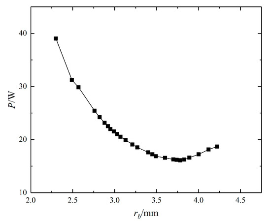
Figure 9.
Optimal total pumping power consumption under different rb.
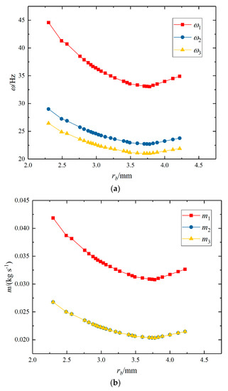
Figure 10.
(a) Optimal frequencies of VSPs. (b) Optimal mass flow rates in loops under different rb.
The variations of the heat transfer area of the evaporator and overall heat transfer coefficients in the system are also investigated. The heat transfer area of evaporator A3, versus the semi-minor axis of elliptical tubes rb is presented in Figure 11. It is found that A3 increases linearly versus rb approximately. Therefore, it can be predicted that the overall heat transfer coefficient of the evaporator k3, will also be affected by the geometry optimization, and has a different variation trend comparing to the overall heat transfer coefficients of heat exchanger HX1 and HX2.
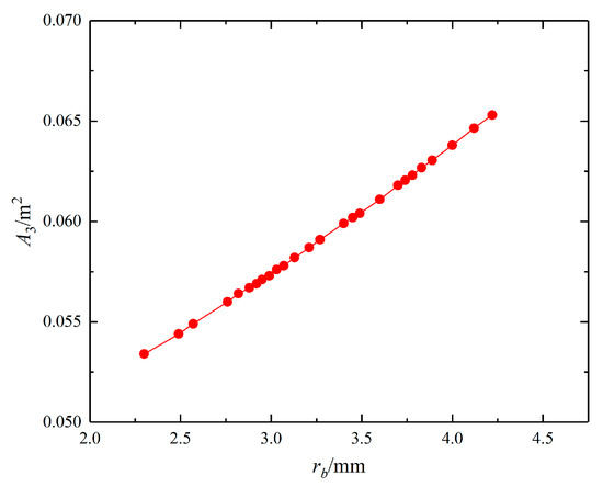
Figure 11.
Heat transfer area of the evaporator under different rb.
Figure 12 shows three overall heat transfer coefficients k1, k2 and k3 under different rb, and the variation trends do match the prediction. Overall heat transfer coefficients of HX1 and HX2, i.e., k1 and k2, are merely determined by operation parameters via heat transfer correlations [34], since their geometry and structure parameters remain unchanged. Therefore, the variation trend of k1 and k2 corresponds to the trend of pump frequencies ω1 and ω2 as well as mass flow rates m1 and m2. However, the overall heat transfer coefficient of the evaporator k3, presents a different variation mode. When the semi-minor axis rb > 3.75 mm, the mass flow rate in the tube decreases with rb decreases, which weakens the heat transfer performance of the evaporator. On the other hand, the decrease of rb would strengthen the heat transfer in the tube comparing to round tubes. The competition of two factors together derives a slowly increasing overall heat transfer coefficient k3 with a decreasing rb. Meanwhile, when the semi-minor axis rb ≤ 3.75 mm, the mass flow rate m3 increases with a decreasing rb. In this case the two factors do not compete but result in a strengthened heat transfer performance, and the overall heat transfer coefficient k3 increases significantly with a decreasing rb.
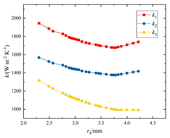
Figure 12.
Overall heat transfer coefficients of heat exchangers under different rb.
Recall that in the physical picture presented by heat current method, heat flows from the hot end to cold end through thermal resistances, which describe heat transfer ability of components. In this system, the pressure drop in the evaporator is far smaller comparing to pressure drops in HX1 and HX2, and hence it only has a negligible effect on the system performance optimization. Therefore, the variation trend of the system optimization result is mainly determined by the trade-off relation between the heat transfer area and the overall heat transfer coefficient of the evaporator. More specifically, the optimal result is generated from the trade-off between the heat transfer enhancement due to the increase of mass flow rate and due to the shape variation of tubes.
Although a rather simple multi-loop heat transfer system is adopted in this study as an example, the proposed synergetic optimization framework is not limited to this case. Recent studies have shown that heat current method can be used for heat transfer systems with different complicated topology structures and even for complex thermodynamic systems. Besides, component design optimization and local heat transfer process optimization also work for other heat exchangers. Therefore, the proposed optimization method here is not limited by specific topology structures of heat transfer systems but has a wide application scope.
5. Conclusions
Optimization of heat transfer systems benefits energy efficiency. In this study, a synergetic optimization method combining system-level optimization, component design optimization, and local heat transfer process optimization is proposed. The system-level optimization is implemented by the heat current method and hydraulic analysis, the component design optimization of the evaporator is performed using the downhill simplex algorithm, and the simulation of heat exchangers uses CFD computation. The local convective heat transfer process in the evaporator is optimized by the field synergy principle, where an additional volume force is introduced to obtain the optimal flow field. These three levels are integrated by using the proposed iterating and updating strategy to provide self-consistent and credible results such as heat transfer coefficients and pressure drops in the system.
A typical multi-loop HTS is optimized to minimize pumping power consumption using the proposed method as an example. The optimization results present that there exists an optimal value for the semi-minor axis rb for elliptical tubes in the evaporator, and the optimal value of rb is 3.75 mm. The optimal flow field in the elliptical tubes can be obtained by designing of the inner surface shape of tubes in practical applications. Besides, the synergetic optimization gives a 16.2 W total pump consumption, which is a 16.3% saving comparing the results without component design optimization. Therefore, the synergetic optimization including component design optimization is more efficient to optimize the system performance. The coupled relation between the system optimization, geometry design optimization, and local heat transfer process optimization can be properly handled by the iterating and updating process. On the other hand, optimization results under different semi-minor axis rb presents that the optimum rb is the result of two competing mechanisms of heat transfer performance enhancement. That is, the optimal rb is determined by the trade-off relation between heat transfer enhancement due to the mass flow rate increase and due to the shape variation of the tube. Finally, since the proposed method relies on the heat current method and CFD simulation as well as the iteration strategy, it is not limited in this pure heat transfer case and could be applied to various other thermal systems even integrated energy systems. Therefore, the proposed method has a wide application scope and would benefit the thermal system optimization.
Author Contributions
Conceptualization, Q.C.; methodology, D.L. and T.Z.; software, D.L.; validation, T.Z., K.-L.H., and X.C.; investigation, D.L., K.-L.H., and T.Z.; data curation, D.L.; writing—original draft preparation, T.Z.; writing—review and editing, T.Z. and Q.C.; visualization, D.L.; supervision, Q.C.; funding acquisition, Q.C. All authors have read and agreed to the published version of the manuscript.
Funding
This research was funded by the National Natural Science Foundation of China, grant number 51836004.
Conflicts of Interest
The authors declare no conflict of interest.
Appendix A. Partial Derivatives in Lagrange Equations
The partial derivatives of thermal resistances with respect to mass flow rates used in the Lagrange equations are as follows:
References
- Bordin, C.; Gordini, A.; Vigo, D. An optimization approach for district heating strategic network design. Eur. J. Oper. Res. 2016, 252, 296–307. [Google Scholar] [CrossRef]
- Ponce-Ortega, J.M.; Jimenez-Gutierrez, A.; Grossmann, I.E. Optimal synthesis of heat exchanger networks involving isothermal process streams. Comput. Chem. Eng. 2008, 32, 1918–1942. [Google Scholar] [CrossRef]
- Adjiman, C.S.; Androulakis, I.P.; Floudas, C.A. Global optimization of mixed-integer nonlinear problems. AIChE J. 2000, 46, 1769–1797. [Google Scholar] [CrossRef]
- Ravagnani, M.; Silva, A.; Arroyo, P.; Constantino, A. Heat exchanger network synthesis and optimisation using genetic algorithm. Appl. Therm. Eng. 2005, 25, 1003–1017. [Google Scholar] [CrossRef]
- Sameti, M.; Haghighat, F. Optimization approaches in district heating and cooling thermal network. Energy Build. 2017, 140, 121–130. [Google Scholar] [CrossRef]
- Bejan, A. Entropy generation minimization: The new thermodynamics of finite-size devices and finite-time processes. J. Appl. Phys. 1996, 79, 1191–1218. [Google Scholar] [CrossRef]
- Tsatsaronis, G.; Moran, M.J. Exergy-aided cost minimization. Energy Convers. Manag. 1997, 38, 1535–1542. [Google Scholar] [CrossRef]
- Lavric, V.; Baetens, D.; Pleşu, V.; De Ruyck, J. Entropy generation reduction through chemical pinch analysis. Appl. Therm. Eng. 2003, 23, 1837–1845. [Google Scholar] [CrossRef]
- Ahmadi, P.; Rosen, M.A.; Dincer, I. Multi-objective exergy-based optimization of a polygeneration energy system using an evolutionary algorithm. Energy 2012, 46, 21–31. [Google Scholar] [CrossRef]
- Kerdan, I.G.; Raslan, R.; Ruyssevelt, P. An exergy-based multi-objective optimisation model for energy retrofit strategies in non-domestic buildings. Energy 2016, 117, 506–522. [Google Scholar] [CrossRef]
- Song, C.; Tan, S.; Qu, F.; Liu, W.; Wu, Y. Optimization of mixed refrigerant system for LNG processes through graphically reducing exergy destruction of cryogenic heat exchangers. Energy 2019, 168, 200–206. [Google Scholar] [CrossRef]
- Marty, F.; Serra, S.; Sochard, S.; Reneaume, J.-M. Exergy Analysis and Optimization of a Combined Heat and Power Geothermal Plant. Energies 2019, 12, 1175. [Google Scholar] [CrossRef]
- Zhang, Y.; Wei, Z.; Wang, X. Inverse problem and variation method to optimize cascade heat exchange network in central heating system. J. Therm. Sci. 2017, 26, 545–551. [Google Scholar] [CrossRef]
- Chen, Q.; Hao, J.; Zhao, T. An alternative energy flow model for analysis and optimization of heat transfer systems. Int. J. Heat Mass Transf. 2017, 108, 712–720. [Google Scholar] [CrossRef]
- Chen, X.; Chen, Q.; Chen, H.; Xu, Y.-G.; Zhao, T.; Hu, K.; He, K.-L. Heat current method for analysis and optimization of heat recovery-based power generation systems. Energy 2019, 189, 116209. [Google Scholar] [CrossRef]
- Zhao, T.; Min, Y.; Chen, Q.; Hao, J. Electrical circuit analogy for analysis and optimization of absorption energy storage systems. Energy 2016, 104, 171–183. [Google Scholar] [CrossRef]
- Chen, Q.; Zhao, T. Heat recovery and storage installation in large-scale battery systems for effective integration of renewable energy sources into power systems. Appl. Therm. Eng. 2017, 122, 194–203. [Google Scholar] [CrossRef]
- Wei, H.; Ge, Z.; Yang, L.; Du, X. Entransy based optimal adjustment of louvers for anti-freezing of natural draft dry cooling system. Int. J. Heat Mass Transf. 2019, 134, 468–481. [Google Scholar] [CrossRef]
- Shao, W.; Chen, Q.; Zhang, M.-Q. Operation optimization of variable frequency pumps in compound series-parallel heat transfer systems based on the power flow method. Energy Sci. Eng. 2018, 6, 385–396. [Google Scholar] [CrossRef]
- Ahmadi, P.; Hajabdollahi, H.; Dincer, I. Cost and Entropy Generation Minimization of a Cross-Flow Plate Fin Heat Exchanger Using Multi-Objective Genetic Algorithm. J. Heat Transf. 2010, 133, 1–10. [Google Scholar] [CrossRef]
- Xie, G.; Song, Y.; Asadi, M.; Lorenzini, G. Optimization of Pin-Fins for a Heat Exchanger by Entropy Generation Minimization and Constructal Law. J. Heat Transf. 2015, 137, 1–9. [Google Scholar] [CrossRef]
- Misra, R.; Jakhar, S.; Agrawal, K.K.; Sharma, S.; Jamuwa, D.K.; Soni, M.S.; Das Agrawal, G. Field investigations to determine the thermal performance of earth air tunnel heat exchanger with dry and wet soil: Energy and exergetic analysis. Energy Build. 2018, 171, 107–115. [Google Scholar] [CrossRef]
- Valencia, G.; Núñez, J.; Duarte, J. Multiobjective Optimization of a Plate Heat Exchanger in a Waste Heat Recovery Organic Rankine Cycle System for Natural Gas Engines. Entropy 2019, 21, 655. [Google Scholar] [CrossRef]
- Li, K.; Wen, J.; Liu, Y.; Liu, H.; Wang, S.; Tu, J. Application of entransy theory on structure optimization of serrated fin in plate-fin heat exchanger. Appl. Therm. Eng. 2020, 173, 114809. [Google Scholar] [CrossRef]
- Wang, S.; Xiao, B.; Ge, Y.; He, L.; Li, X.; Liu, W.; Liu, Z. Optimization design of slotted fins based on exergy destruction minimization coupled with optimization algorithm. Int. J. Therm. Sci. 2020, 147, 106133. [Google Scholar] [CrossRef]
- Li, L.; Wan, H.; Gao, W.; Tong, F.; Li, H. Reliability based multidisciplinary design optimization of cooling turbine blade considering uncertainty data statistics. Struct. Multidiscip. Optim. 2018, 59, 659–673. [Google Scholar] [CrossRef]
- Sahin, A.Z. Second Law Analysis of Laminar Viscous Flow Through a Duct Subjected to Constant Wall Temperature. J. Heat Transf. 1998, 120, 76–83. [Google Scholar] [CrossRef]
- Sahin, A.Z. Thermodynamics of laminar viscous flow through a duct subjected to constant heat flux. Energy 1996, 21, 1179–1187. [Google Scholar] [CrossRef]
- Guo, Z.; Tao, W.; Shah, R. The field synergy (coordination) principle and its applications in enhancing single phase convective heat transfer. Int. J. Heat Mass Transf. 2005, 48, 1797–1807. [Google Scholar] [CrossRef]
- Tao, W.; Guo, Z.-Y.; Wang, B.-X. Field synergy principle for enhancing convective heat transfer––its extension and numerical verifications. Int. J. Heat Mass Transf. 2002, 45, 3849–3856. [Google Scholar] [CrossRef]
- Meng, J.-A.; Liang, X.-G.; Li, Z.-X. Field synergy optimization and enhanced heat transfer by multi-longitudinal vortexes flow in tube. Int. J. Heat Mass Transf. 2005, 48, 3331–3337. [Google Scholar] [CrossRef]
- Chen, Q.; Wang, M.; Pan, N.; Guo, Z.-Y. Optimization principles for convective heat transfer. Energy 2009, 34, 1199–1206. [Google Scholar] [CrossRef]
- Chen, X.; Zhao, T.; Zhang, M.-Q.; Chen, Q. Entropy and entransy in convective heat transfer optimization: A review and perspective. Int. J. Heat Mass Transf. 2019, 137, 1191–1220. [Google Scholar] [CrossRef]
- Rohsenow, W.M.; Hartnett, J.P.; Ganic, E.N.; Richardson, P.D. Handbook of Heat Transfer Fundamentals (Second Edition). J. Appl. Mech. 1986, 53, 232–233. [Google Scholar] [CrossRef]
- Gómez, A.; Montañés, C.; Camara, M.; Cubero, A.; Fueyo, N.; Muñoz, J.M. An OpenFOAM-based model for heat-exchanger design in the Cloud. Appl. Therm. Eng. 2018, 139, 239–255. [Google Scholar] [CrossRef]
- Dogan, S.; Darici, S.; Ozgoren, M. Numerical comparison of thermal and hydraulic performances for heat exchangers having circular and elliptic cross-section. Int. J. Heat Mass Transf. 2019, 145, 118731. [Google Scholar] [CrossRef]
- Zhao, T.; Liu, D.; Chen, Q. A collaborative optimization method for heat transfer systems based on the heat current method and entransy dissipation extremum principle. Appl. Therm. Eng. 2019, 146, 635–647. [Google Scholar] [CrossRef]
- Chung, T.J. Computational Fluid Dynamics, 2nd ed.; Cambridge University Press: Cambridge, UK, 2010; ISBN 978-0-511-78006-6. [Google Scholar]
- Reddy, J.N. Energy Principles and Variational Methods in Applied Mechanics, 3rd ed.; Wiley: Hoboken Chichester, NJ, USA, 2017; ISBN 978-1-119-08737-3. [Google Scholar]
- Barnard, R.W.; Pearce, K.; Schovanec, L. Inequalities for the Perimeter of an Ellipse. J. Math. Anal. Appl. 2001, 260, 295–306. [Google Scholar] [CrossRef]
- Chen, Q.; Liang, X.-G.; Guo, Z. Entransy theory for the optimization of heat transfer—A review and update. Int. J. Heat Mass Transf. 2013, 63, 65–81. [Google Scholar] [CrossRef]
- Liu, D.; Chen, Q.; He, K.-L.; Chen, X. An integrated system-level and component-level optimization of heat transfer systems based on the heat current method. Int. J. Heat Mass Transf. 2019, 131, 623–632. [Google Scholar] [CrossRef]
- Hamid, M.O.; Zhang, B.; Yang, L. Application of field synergy principle for optimization fluid flow and convective heat transfer in a tube bundle of a pre-heater. Energy 2014, 76, 241–253. [Google Scholar] [CrossRef]


© 2020 by the authors. Licensee MDPI, Basel, Switzerland. This article is an open access article distributed under the terms and conditions of the Creative Commons Attribution (CC BY) license (http://creativecommons.org/licenses/by/4.0/).