Influence of the Thermometer Inertia on the Quality of Temperature Control in a Hot Liquid Tank Heated with Electric Energy

Abstract

This paper presents the medium temperature monitoring system based on digital proportional–integral–derivative (PID) control. For industrial thermometers with a complex structure used for measuring the temperature of the fluid under high pressure, the accuracy of the first-order model is inadequate. A second-order differential equation was applied to describe a dynamic response of a temperature sensor placed in a heavy thermowell (industrial thermometer). The quality of the water temperature control system in the tank was assessed when measuring the water temperature with a jacketed thermocouple and a thermometer in an industrial casing. A thermometer of a new design with a small time constant was also used to measure temperature. The quality of water temperature control in the hot water storage tank was evaluated using a classic industrial thermometer and a new design thermometer. In both cases, there was a K-type sheathed thermocouple inside the thermowell. Reductions in the time constant of the new thermometer are achieved by means of a steel casing with a small diameter hole inside which the thermocouple is precisely fitted. The time constants of the thermometers were determined experimentally with a jump in water temperature. A digital controller was designed to maintain the preset temperature in an electrically heated hot water tank. The function of the regulator was to adjust the power of the electrical heater to maintain a constant temperature of the liquid in the tank.

1. Introduction

Temperature measurement is the largest segment of all industrial measurements and can often have the most significant impact on process efficiency, energy consumption, and product quality.

High temperature, pressure, and process vibrations make robust temperature measurement devices essential for industrial applications. Besides, high accuracy, repeatability, and stability of temperature measurement are essential to ensure effective process control. A small measurement error can cause numerous disturbances or be very costly, so temperature measurements must be accurate and reliable. For this reason, every measuring system must be carefully designed and also subjected to rigorous control to meet process requirements.

Although many types of temperature sensors can be used, resistance temperature sensors and thermoelectric sensors are most commonly used in the industry [1]. The accuracy of thermocouples is influenced by several factors, including the type of thermocouple, its application range, measuring range, material purity, junction degradation, and manufacturing process [2]. Temperature sensors are very rarely introduced directly into the process line [3]. Most often, they are installed in additional housing [4] to isolate them from potentially harmful process conditions such as flow stress, high pressure, and corrosive chemicals. These housings allow the sensor to be quickly and easily removed from the system for calibration or replacement without stopping the entire process [1,2,3]. However, when using a thermowell, the response time increases significantly due to the increased thermal mass of the unit [5]. The dynamic response time of the sensor can be important when the process temperature changes quickly, and fast inputs to the control system are needed [6]. The basic steps to reduce the reaction time are to reduce the mass of the housing while maintaining adequate mechanical strength to withstand the process pressures and flow forces. Additionally, the reaction time is improved by using a spring-loaded sensor and filling the space in the well with a thermally conductive fluid, thermally conductive ceramic, or thermally conductive sand. The characteristics of the measured medium is also a factor influencing the reaction time, especially concerning its velocity and density.

The paper [7] presents a technique of measurement of the transient temperature of a fluid flowing under high pressure. The temperature inside the thermometer with the sensor in the form of the solid cylinder is measured at its axis to determine the temperature of the fluid. Based on the measured transient temperature in the axis of the cylinder, the inverse problem of heat conduction is solved, and the fluid temperature is determined. Examples of applications of the method developed in [7] are presented in the paper [8]. The safe and high-performance operation of power units requires, among other things, monitoring of thermal, flow, and strength parameters of steam power boilers working under high pressure, at high temperatures, and additionally under load changing in time [9]. It is reasonable to monitor thermal and pressure stresses in thick-walled components of power boilers, such as steam drums, injection chambers of superheated steam spray attemperators, superheater headers during start-up, shutdown, and load change of boilers, to protect critical pressure elements [10]. Monitoring should cover not only pressure elements, such as those mentioned above which are subject to a circular-symmetric temperature distribution or single-phase or two-phase medium, but also thick-walled pressure elements in steam pipelines, such as the main steam gate or the T and Y-junction. The basis is a correctly determined time-space temperature and stress distribution over the entire cross-section of the thick-walled pressure element and a measurement of the medium flowing temperature. The effective method of control of thermal and pressure stresses uses the solution of the inverse heat conduction problem [10]. It is convenient to use in practice since it is based on measuring temperature changes on an external, easily accessible surface without drilling holes in the walls of structural elements [9]. The paper [9] shows that the measurement of transient steam temperature using an industrial thermometer has a substantial error. In the case of the injection of water into the steam stream in a steam cooler (attemporator), the dynamic measurement error reached even 80 K. Due to the long delay and damping of temporary steam temperature changes, the cascade proportional–integral–derivative (PID) system for temperature control does not work properly. Such large dynamic inaccuracies in determining the steam temperature also cause large errors in the indirect determination of thermal stresses [10].

Instruments for measuring the transient temperature of the fluid were also subject to patents. Baerts and van Gerwen proposed the use of the proportional–integral–derivative (PID) controller equation [11] to decrease the dynamic error in gas temperature measurement in the engine outlet. Dietmann and Wienand [12] designed a new thermometer shell for measuring gas temperature between −40 °C and 1000 °C. The tip of the temperature sensor was filled with a ceramic mass having a high thermal conductivity ranging from 0.5 to 3 W/(m·K) [12]. The thermometer is appropriate for high-temperature measurements, but because of the thin casing, the thermometer is unsuitable for the high-pressure fluid at high velocity. At high fluid velocities, the large bending moments act on the thermometer casing, which can damage them.

The subjects of the paper by Monroe et al. [13] are studies of temperature behavior along the adiabatic section of a tubular oscillating heat pipe under operation for varying heat inputs. The temperature changes were controlled with the use of T-type thermoelectric sensors located either inside or along the heat pipe wall in the region between the evaporator and condenser. The measurements were used to evaluate the influence of the thermal capacity of walls, the temperature gradient of external walls, and the internal fluid adsorption. The internal, single-phase heat transfer coefficient was estimated, and the effective thermal conductivity of the projector was determined. It was found that heat conduction through pipe walls constitutes from 2% to 10% of the overall heat transfer coefficient, and significantly decreases with the increase in liquid advection at higher values of heat flow rates.

Optical fiber sensors are widely used in medical monitoring, military engineering, power systems, etc. for accurate measurement and the prediction of temperature and magnetic field intensity. The paper [14] presents research on micro-structured optical fiber as a high-sensitivity sensor with a temperature sensitivity of the nanometer scale and magnetic field of the picometer scale.

Seo et al. [15] proposed a flexible, detachable dual-output sensor for fluid temperature and moving dynamics based on the structural design of thermoelectric materials that detect changes in temperature and moving dynamics of water in high resolutions (<0.19 K and <0.03 cm/s). The authors conducted theoretical analysis and simulations of the structural design of thermoelectric materials (SDTM) modules’ operation, the outcomes of which were compared with the results of experimental research.

Due to the great variety of processes in the industry as well as the different dimensions of the elements whose temperature is measured, various temperature measurement procedures are developed. The paper [16] proposes a method of measuring temperature on the inner surface of a microchannel based on the solution of the inverse problem of heat conduction. Due to the large dimensions of the thermocouple, it is not possible to place it inside the microchannel to measure the temperature of its inner surface. Therefore, the temperature of the easily accessible external surface of the duct is measured, and then the temperature and heat transfer coefficient on the internal surface of the duct is determined from the solution of the inverse problem.

A different approach to the determination of the heat transfer coefficient on the external surface of a mini channel is presented in paper [17]. Infrared thermography was used to avoid the insertion of large temperature sensors into the mini channel to determine the temperature distribution on its external surface. Then, a recovery of the heat transfer coefficient over the mini-channel outer surface and the internal boundary conditions were achieved with the measured temperature distributions and the inverse approach.

Modeling of heat transfer processes in dynamic scraped surface heat exchangers is a very complex problem. The processes in these types of heat exchangers comprise the complex dynamics of the flow of viscous, multi-phase temperature-dependent fluids. Analytical methods to study the mechanisms of liquid and heat transfer in dynamic scraped-surface heat exchangers are limited. To fully characterize the physical phenomena occurring inside the chamber, it is necessary to install an array of temperature and pressure sensors. The paper [18] presents the results of experimental research and computational fluid dynamics (CFD) modeling of such exchangers.

The analysis of factors influencing the process of fuel combustion in bubbling fluidized beds is the subject of the paper [19]. The thermographic camera measurements of temperature distribution in the fluidized bed were used to estimate the influence of key parameters of the process such as fluidization velocity, particle size, and pressure drop over the air distributor plate on the lateral mixing of bulk solids in bubbling fluidized beds. Utilizing the measured pressure drop over the bed, the sampled temperature field, and the finite volume method, the energy conservation equation was discretized at the pixel level. Next, the calculated effective heat transfer coefficient was used to determine the solid dispersion coefficient and solids volumetric fraction in the bed.

Under steady-state conditions, when the liquid temperature is constant, the temperature is measured with high accuracy because there is no damping or delay of the thermometer indications in relation to the medium temperature. When the temperature of a fluid changes rapidly, there are significant differences between the actual temperature of the fluid and the measured temperature. The reason for this is the time needed to transfer the heat to a temperature sensor in a solid casing. The PID (proportional–integral–derivative) is the most commonly used controller in the industry and has been the dominant control technique for process control for many decades [18,19].

The literature review shows that there are no fast response thermometers suitable for high-pressure fluid temperature measurement. The use of massive industrial thermometers in PID control systems results in the faulty operation of these systems, which may cause overheating of the pressure elements and too high a thermal stress and, consequently, decrease the lifetime of these elements.

In the digital PID controller, different mathematical models of thermometers were used to control the fluid temperature. Temperature sensors with a simple structure, such as a sheathed thermocouple, can be treated as inertial objects of the first order. Experimental tests were carried out to determine the time constants used in mathematical models for the thermometers investigated. One time constant is needed for the first order thermometer model and two time constants for the second-order model.

In this work, a digital PID control was developed to maintain a constant temperature in the domestic hot water tank. The electric heater raises the temperature of the water in the tank. A lumped capacity mathematical model of a hot water tank was developed, taking into account heat losses on the outer surface of the container. A second-order ordinary differential equation with two time constants describes the temporal changes of the temperature indicated by the thermometer. The time constants of the thermometer were pre-determined experimentally. The second-order equation for the thermometer was replaced by a system of two ordinary first-order differential equations to increase the accuracy of the numerical temperature determination of the thermometer. Thus, the time variations of the water and thermometer temperatures are described by a system of three first-order ordinary differential equations. The initial problem for the system of ordinary differential equations was solved by the Runge–Kutta method of the fourth order.

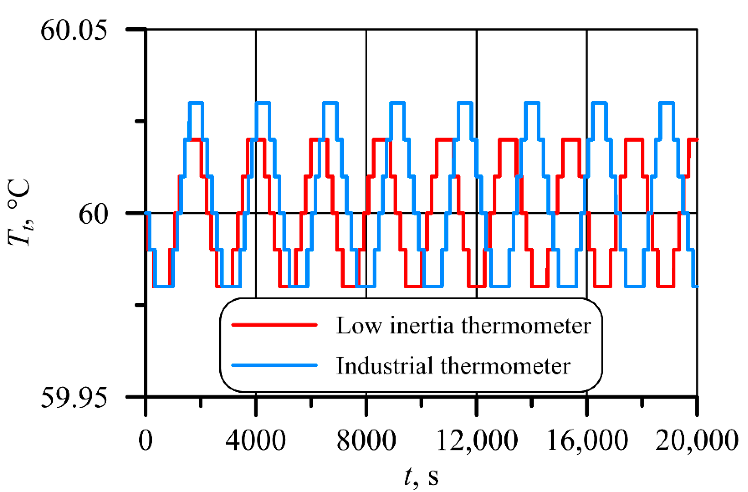
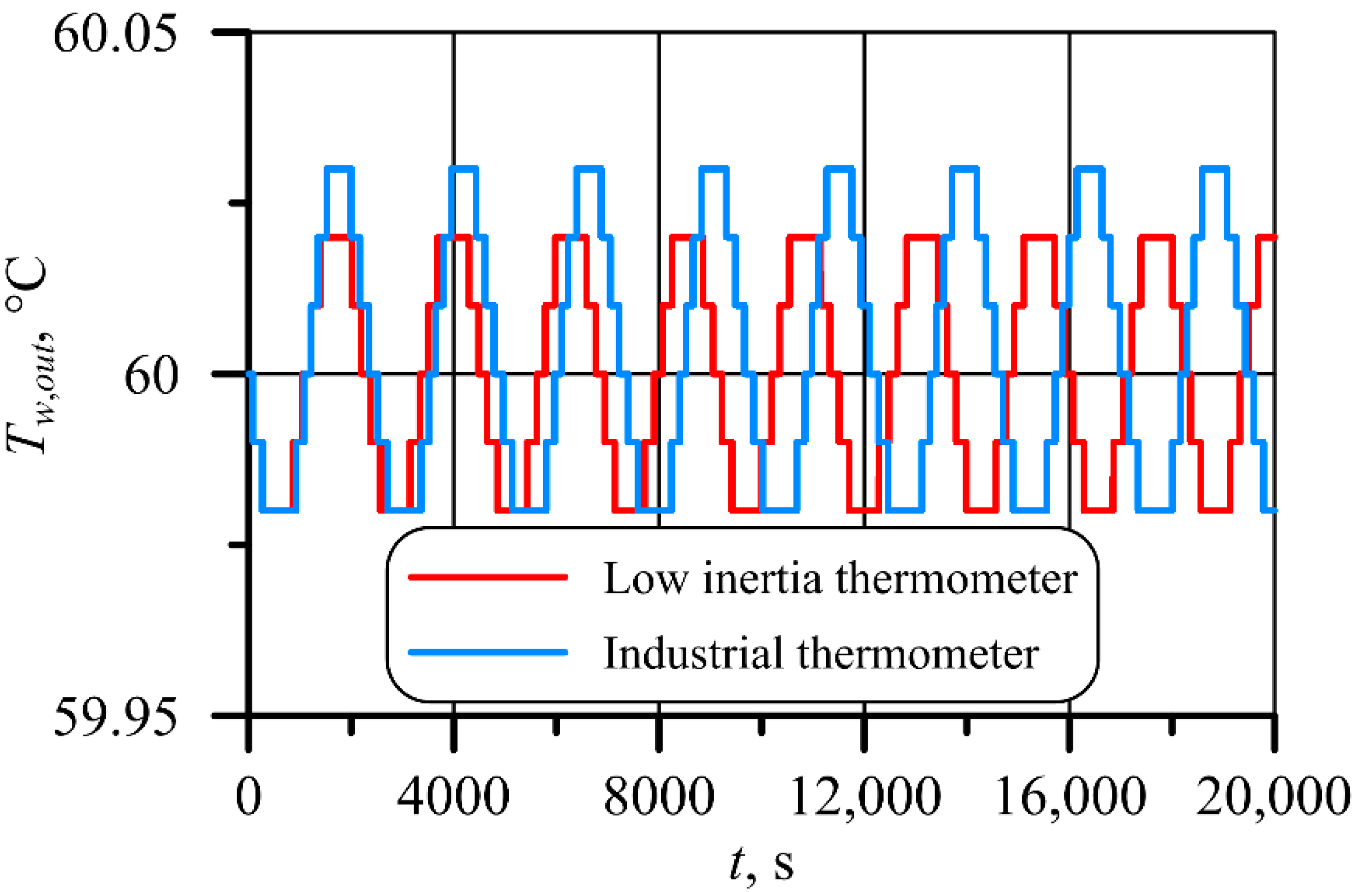
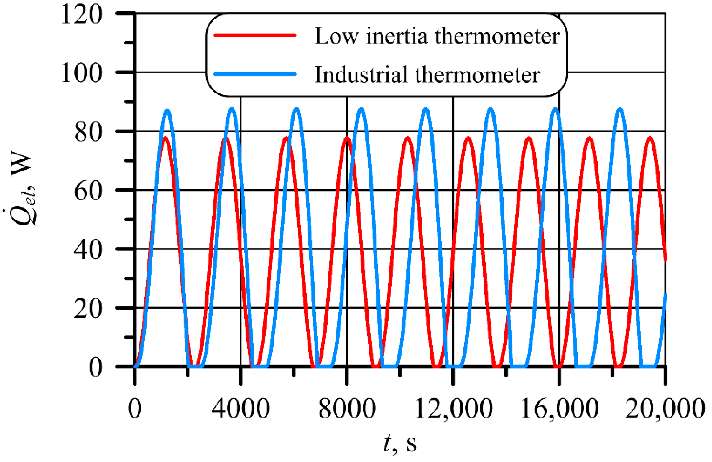
The task of the digital PID controller is to maintain the set temperature in the tank. It was shown that the new design thermometer, characterized by low inertia, contributes to faster achievement of the set temperature in the tank.

The use of a fast response thermometer reduces the electricity consumption for maintaining constant water temperature in the tank. Over one month and longer, these savings are noticeable. A digital PID control system has been developed, which operates online without large financial outlays. An important new element in this system is the use of a second-order inertial model to describe the dynamics of a complex thermometer. The second-order inertial model takes into account the delay of the thermometer reading in relation to changes in liquid temperature.

The main aim of the article was to compare the PID temperature control system using an industrial thermometer and a fast response thermometer developed by the authors. Ultimately, the low inertia thermometer will be used in temperature control systems for steam or gas with high temperature and pressure flowing at high velocity. Currently, massive thermometers are used [9,10], which prevent proper operation of the cascade PID regulation used to maintain the set temperature of superheated steam.

The novelty of the article is a numerical model of the thermometer tank system, which allows for the simulating of the operation of the PID control system. Simulations carried out with the use of a digital PID controller show that in the case of an object with a very high thermal inertia, the influence of the thermometer’s inertia on the quality of control is not great. Much better effects of PID controller operation can be obtained, e.g., in case of large steam superheaters in power boilers, because the superheater’s time constant is shorter and differences between industrial and new thermometer inertia are much bigger [9,10].

2. Mathematical Model of the Thermometer and Water Storage Tank

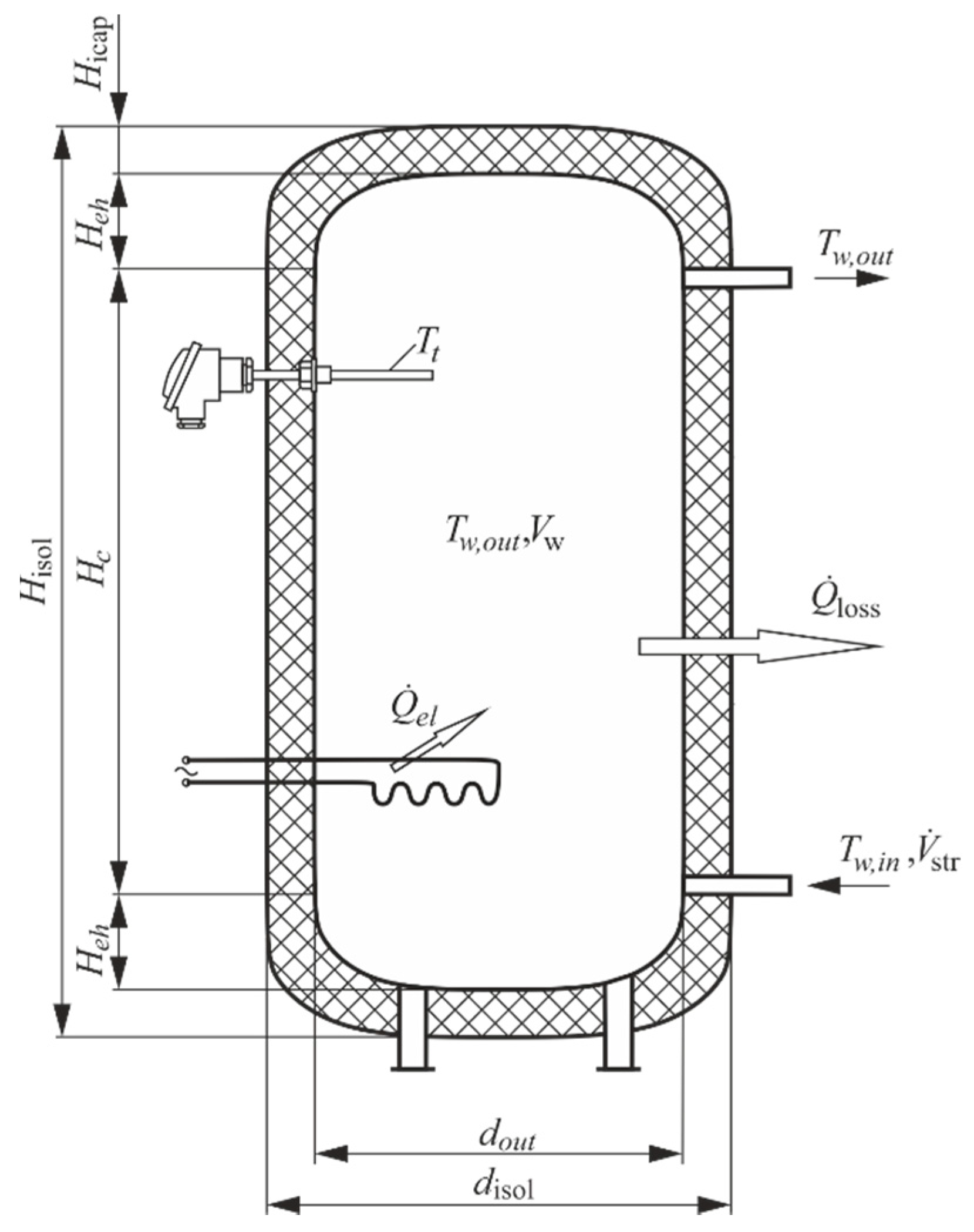
PID control systems are also widely used in the energy sector and many other industries. The operation of PID systems in temperature control of high pressure and temperature fluids is often faulty due to the high inertia of thermometers. The novelty of the paper is to develop a dynamic mathematical model of the system to analyze the operation of a PID control system with a conventional industrial thermometer and a newly designed low inertia thermometer. The digital PID control of temperature in the hot water tank will be shown. The heat storage tank is depicted in Figure 1.

The following assumptions were made in the construction of a mathematical model of a hot water tank with thermometers:

• the temperature of the water in the tank is uniform and depends only on time,
• the time-dependent temperature of the water and steel wall of the tank are identical,
• the tank was modelled as a body with lumped thermal capacity at the temperature T_w,out(t) (Figure 1),
• the heat transfer coefficients on the inner surface of the tank and the outer surface of the insulation are constant,
• an industrial thermometer, as well as a fast response thermometer, were modeled as inertial objects of the second order.

The energy conservation equation for the hot water tank has the following form

$$\left(V_w{\rho }_w{c}_w+m_m{c}_m\right)\frac{d{T}_{w,out}}{dt}={\dot{V}}_{str}{\rho }_w{c}_w{T}_{w,in}-{\dot{V}}_{str}{\rho }_w{c}_w{T}_{w,out}+{\dot{Q}}_{el}-{\dot{Q}}_{loss}$$

(1)

where ρ_w—denotes water density, kg/m³, c_w—water specific isobaric heat capacity, J/(kg·K), m_m—the mass of the storage tank, kg, c_m—stainless steel specific heat capacity, J/(kg·K), T_w,in—inlet water temperature, °C, T_w,out—outlet and storage tank water temperature, °C, ${\dot{Q}}_{el}$—heat flow rate transferred from an electric heater to water, W, and ${\dot{Q}}_{loss}$—heat losses to the environment, W.

By converting the last equation for the time derivative of the water temperature, one obtains

$$\frac{d{T}_{w,out}}{dt}=\frac{{\dot{V}}_{str}{\rho }_w{c}_w}{\left(V_w{\rho }_w{c}_w+m_m{c}_m\right)}\left(T_{w,in}-T_{w,out}\right)+\frac{{\dot{Q}}_{el}-{\dot{Q}}_{loss}}{\left(V_w{\rho }_w{c}_w+m_m{c}_m\right)}$$

(2)

Equation (2) gives the rate of change of the water temperature. The heat flow to the environment (heat loss to the surroundings) is calculated as follows

$${\dot{Q}}_{loss}=U_{in}{A}_{in}\left(T_{w,out}-T_{env}\right)$$

(3)

where A_in is the area of the storage tank inner surface, m², and U_in is the overall heat transfer coefficient referred to the inner surface of the tank

$$\frac{1}{U_{in}}=\frac{1}{h_{in}}+\frac{2A_{in}}{A_{in}+A_{out}}\frac{{\delta }_m}{k_m}+\frac{2A_{in}}{A_{out}+A_{isol}}\frac{{\delta }_{isol}}{k_{isol}}+\frac{A_{in}}{A_{isol}}\frac{1}{h_{out}}$$

(4)

The heat flux ${\dot{q}}_{in}$ at the inner surface of the tank is given by

$${\dot{q}}_{in}=\frac{{\dot{Q}}_{loss}}{A_{in}}=U_{in}\Delta T=\frac{\mathsf{\Delta }T}{{\displaystyle \sum R_{thermal}}}=\frac{T_{w,out}-T_{env}}{R_{in}+R_{wall}+R_{isol}+R_{out}}$$

(5)

where

$$R_{in}=\frac{1}{h_{in}},\hspace{1em}{R}_{wall}=\frac{2A_{in}}{A_{in}+A_{out}}\frac{{\delta }_m}{k_m},\hspace{1em}{R}_{isol}=\frac{2A_{in}}{A_{out}+A_{isol}}\frac{{\delta }_{isol}}{k_{isol}},\hspace{1em}{R}_{out}=\frac{A_{in}}{A_{isol}}\frac{1}{h_{out}}$$

(6)

The symbols R_in, R_wall, R_isol, and R_out in Equations (5) and (6) denote, respectively, inner convective thermal resistance, the conductive thermal resistance of the tank wall, the conductive thermal resistance of the insulation, and outer convective thermal resistance. The thermal circuit for heat flow from hot water through a metal tank wall and thermal insulation to the environment is illustrated in Figure 2.

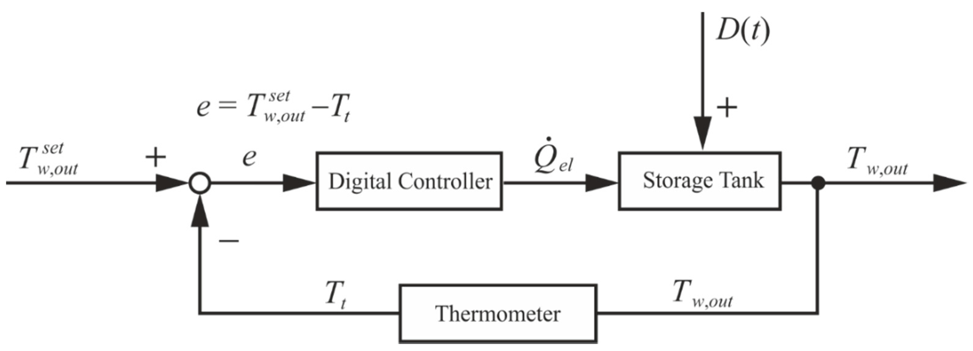
An industrial thermometer was used to control the temperature in the water tank. Due to its complex construction and massive housing, the thermometer was modeled as a second-order inertial object. The second-order ordinary differential equation was used to describe its transient behavior

$${\tau }_1{\tau }_2\frac{d^2{T}_t\left(t\right)}{d{t}^2}+\left({\tau }_1+{\tau }_2\right)\frac{d{T}_t\left(t\right)}{dt}+T_t\left(t\right)=T_{w,out}\left(t\right)$$

(7)

where τ₁ and τ₂ denotes the thermometer time constants. The symbols T_t and T_w,out stand for the temperature indicated by the thermometer and water temperature, respectively.

The second-order differential Equation (7) was replaced by a system of two first-order differential equations

$$\frac{d{T}_t}{dt}=V$$

(8)

$$\frac{dV}{dt}=\frac{1}{{\tau }_1{\tau }_2}\left(T_{w,out}-T_t\right)-\frac{{\tau }_1+{\tau }_2}{{\tau }_1{\tau }_2}V$$

(9)

The set of three ordinary differential Equations (2), (8) and (9) is subject to the following initial conditions

$${T_{w,out}|}_{t=0}=T_0$$

(10)

$${T_t|}_{t=0}=T_0$$

(11)

$${\frac{d{T}_t}{dt}|}_{t=0}=V_0$$

(12)

where: T₀—the initial water and thermometer temperature, V₀—initial value of the thermometer temperature rate.

The mathematical model of the storage tank and the thermometer consisting of Equation (2) for the tank and two Equations (8) and (9) for the thermometer was solved by the Runge–Kutta fourth-order method. For numerical solving of ordinary differential equations, various methods can be used, such as one-step methods, for example, the explicit and implicit Euler methods with the first order of accuracy, or the Runge–Kutta method, and the multi-step methods, for instance, the Milne or Adams–Moulton method [20]. The Euler methods are simple and can be used for non-linear initial value problems. On the other hand, they are less accurate. The approximation error is proportional to the step size. A good approximation is obtained with a very small step size leading to more considerable computation time. The Milne method is simple, but it is subject to an instability problem in certain cases. The Adams–Moulton method does not have the instability problem as the Milne method but requires a set of starting values calculated by some other technique. The fourth-order Runge–Kutta methods are widely used in computer solutions to differential equations. The classic Runge–Kutta methods have proven themselves of substantial value and power for a broad range of scientific and engineering problems. They are easy to implement, explicit, very stable, fast, and self-starting. The fourth-order Runge–Kutta method is computationally more efficient than the Euler and other methods because the steps can be many times greater for the same accuracy. The primary disadvantages of Runge–Kutta methods are that they require significantly more computer time than multi-step methods of comparable accuracy [21].

The developed mathematical model of the water reservoir system including the thermometer simulated the transient behavior of the real system and was used in the digital PID control system.

3. PID Controller

PID regulators are the most commonly used regulators in industrial practice [22,23]. In this paper, the temperature of the water in the storage tank is regulated using a digital PID controller (Figure 3).

The PID controller is designed to keep the temperature of the water in the tank constant. The electrical power of the heater u = ${\dot{Q}}_{el}$ is selected in successive time steps so that the difference between the set temperature $T_{w,out}^{set}$ and the temperature of the thermometer T_t, i.e., $e=T_{w,out}^{set}-T_t$ was equal to zero.

The PID regulator equation has the following form [23]:

$$u\left(t\right)=\overline{u}+K_p\left[e\left(t\right)+\frac{1}{{\tau }_i}{\displaystyle \int e\left(t\right)dt}+{\tau }_d\frac{de\left(t\right)}{dt}\right]$$

(13)

Equation (13) can be written as

$$u\left(t\right)=\overline{u}+K_p\left[e\left(t\right)+K_i{\displaystyle \underset{0}{\overset{t}{\int }}e\left(t\right)dt}+K_d\frac{de\left(t\right)}{dt}\right]$$

(14)

where: u(t)—the output from the controller, t—time, s, $\overline{u}$—average output from the controller, K_p—the proportional gain of the PID controller, e(t)—the difference between the preset and actual measured value, τ_i—integration time, s, τ_d—differential time, s, K_i—the integral gain of the PID controller, s⁻¹, and K_d—the derivative gain of the PID controller, s.

Equation (14) can be rewritten in a discrete form. The integral in the regulator equation is calculated approximately using the rectangles method, and the derivative is replaced by the backward finite-difference. The use of the backward difference results in a simple formula for calculating the u_k value, without the need for iterative calculations. At the time point t_k, the value of the output signal u_k is

$$u_k=\overline{u}+K_p\left(e_k+K_i\Delta t{\displaystyle \sum _{i=1}^k{e}_i}+K_d\frac{e_k-e_{k-1}}{\Delta t}\right), k=1, 2, \dots$$

(15)

where: u_k = u(t_k), e_k = e(t_k), t_k = kΔt, k = 1,2, …

Subsequently, u_k−1 for the time t_k−1 can be expressed as

$$u_{k-1}=\overline{u}+K_p\left(e_{k-1}+K_i\Delta t{\displaystyle \sum _{i=1}^{k-1}{e}_i}+K_d\frac{e_{k-1}-e_{k-2}}{\Delta t}\right)$$

(16)

Subtracting Equation (16) from Equation (15) results in

$$u_k-u_{k-1}=K_p\left(e_k-e_{k-1}+K_i\Delta t\hspace{0.17em}{e}_k+K_d\frac{e_k-2e_{k-1}+e_{k-2}}{\Delta t}\right)$$

(17)

The transformation of Equation (17) leads to an equation used in further calculations

$$u_k=u_{k-1}+K_p\left(e_k-e_{k-1}+K_i\Delta t\hspace{0.17em}{e}_k+K_d\frac{e_k-2e_{k-1}+e_{k-2}}{\Delta t}\right), k=1, 2, \dots$$

(18)

Equation (18) is the basis for the operation of a digital PID controller.

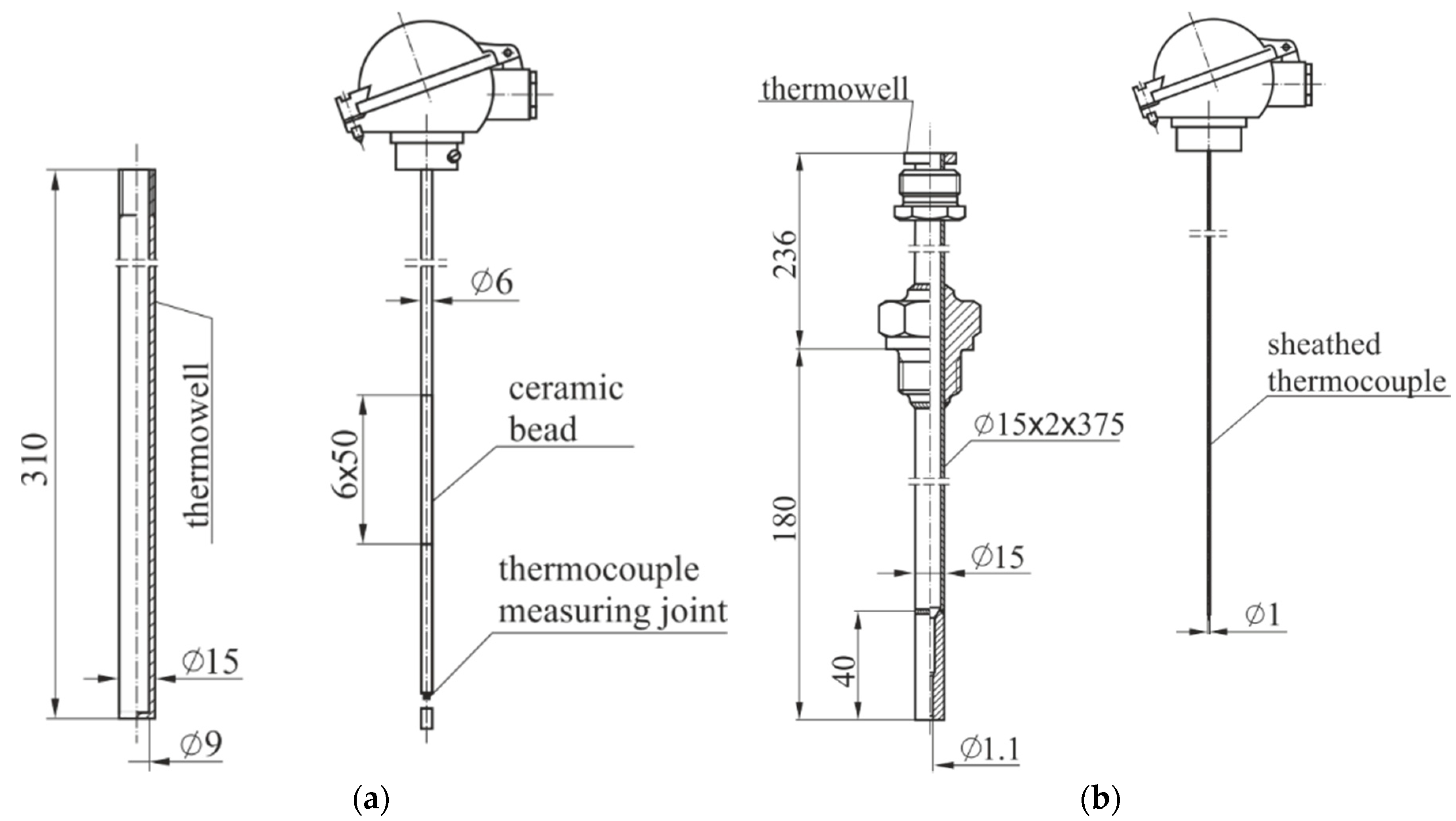
4. Determination of Time Constants of Thermometers Used to Measure Water Temperature

Two different thermometers that can be used to measure the water temperature in the tank were analyzed (Figure 4). A classic industrial thermometer is presented in Figure 4a. The sheathed thermocouple is isolated from the housing with ceramic cylinders. The space between the outer surface of ceramic cylinders and the inner surface of the housing is filled with a bulk porous material, which provides additional thermal resistance. For this reason, an industrial thermometer of classic design has high thermal inertia characterized by a delay of the thermometer indications in relation to the changes of the liquid temperature.

Due to the delayed response of the thermometer, a second-order mathematical model with two time constants was used. The thermometer shown in Figure 4b has much better dynamic properties, with the inner jacket thermocouple well attached to the inner casing. The quality of water temperature control in the hot water storage tank was evaluated using a classic industrial thermometer and a new design thermometer. In both cases, there was a K-type sheathed thermocouple inside the thermowell. Reductions in the time constant of the new thermometer are achieved by means of a steel casing with a small diameter hole inside which the thermocouple is precisely fitted. The diameter of the thermocouple sheath was 1 mm. The casing, together with the thermocouple, was treated as a solid steel cylinder in the axis of which time changes in temperature are known. The dynamic properties of the thermometer in Figure 4b will also be represented by two time constants.

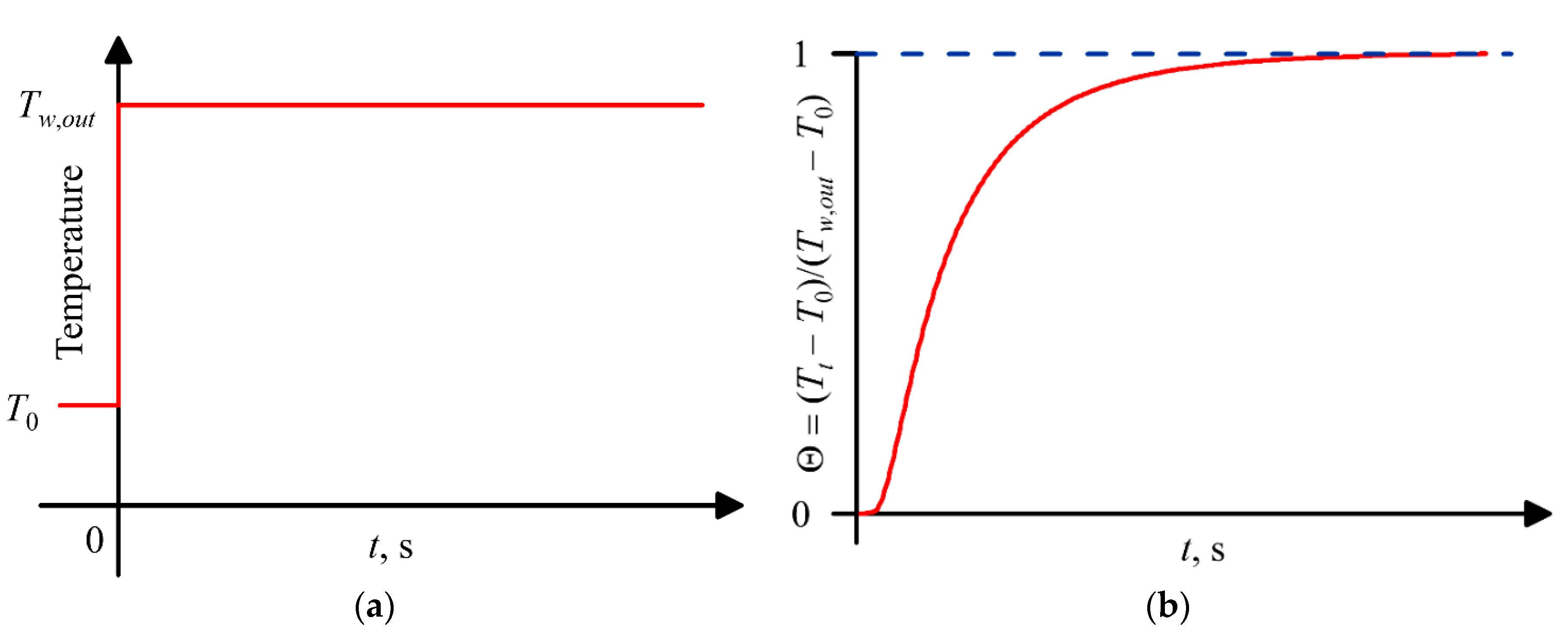
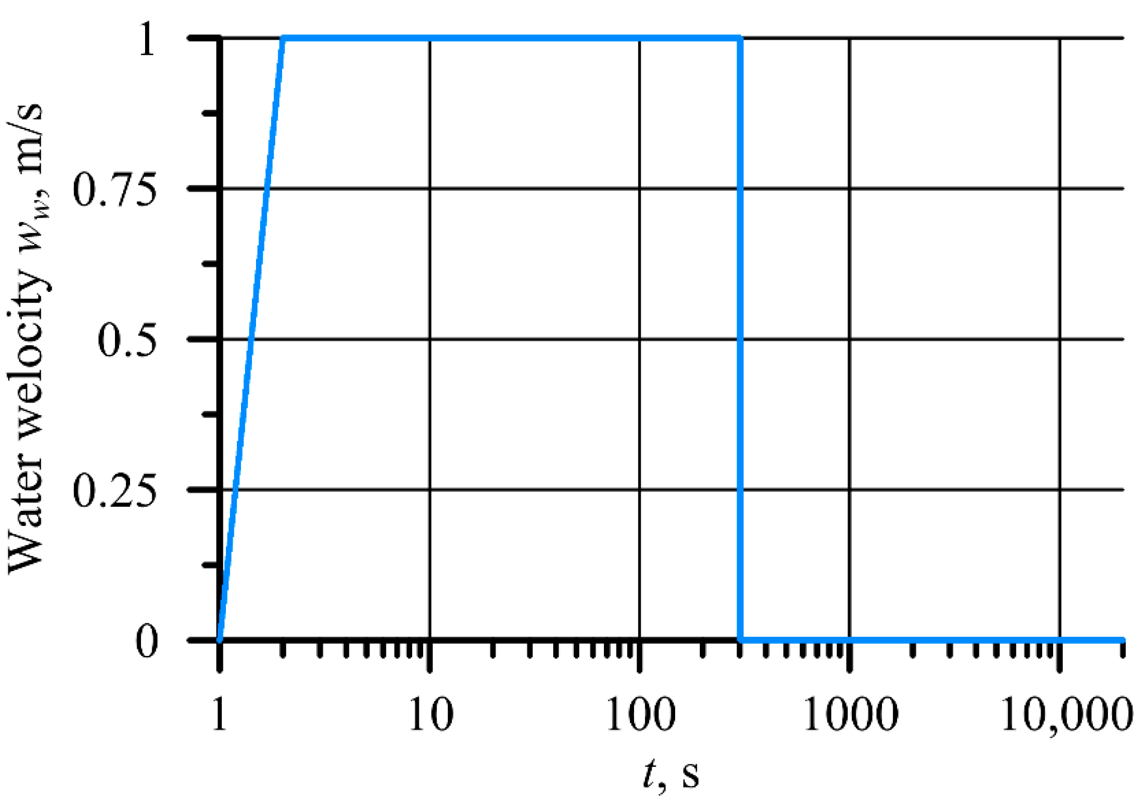
For the experimental determination of the time constants τ₁ and τ₂, Equation (7) was solved with a stepwise change in water temperature (Figure 5a). This solution has the following form

$$\Theta =\frac{T_t-T_0}{T_{w,out}-T_0}=1+\frac{{\tau }_1}{{\tau }_2-{\tau }_1}\exp \left(-\frac{t}{{\tau }_1}\right)-\frac{{\tau }_2}{{\tau }_2-{\tau }_1}\exp \left(-\frac{t}{{\tau }_2}\right)$$

(19)

A diagram of the thermometer response to unit jump (Heaviside function) in liquid temperature is shown in Figure 5b. A sudden change of the ambient temperature was realized by sudden insertion of the thermometer with the initial temperature T₀ into hot water of T_w,out temperature.

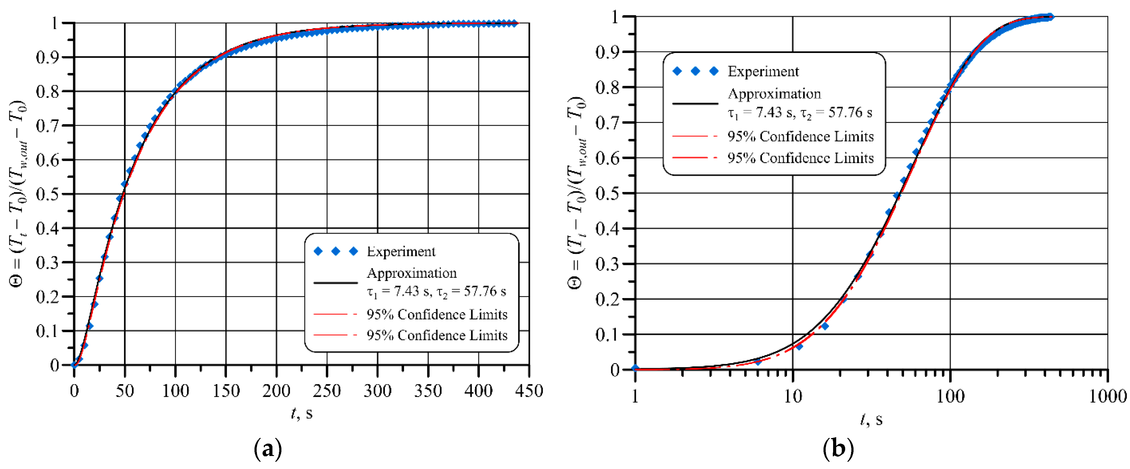
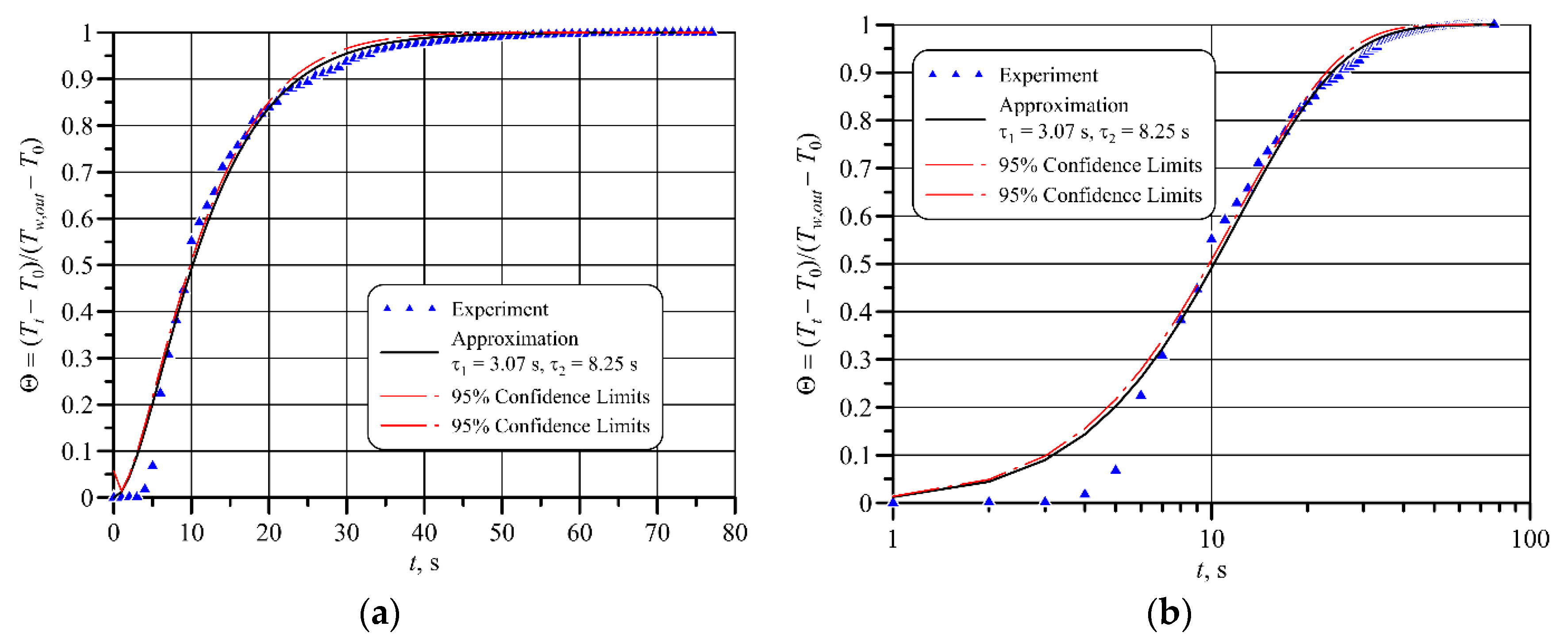
The temperature of the thermometer was measured in a few hundred points. Sampling time was 1 s. Thermometer temperatures T_t (t_i), i = 1, 2, ..., n_t measured at time points were approximated by Equation (19) using the least-squares method [24]. The values of time constants τ₁ and τ₂, at which the sum of squares of temperature differences between the temperature indicated by the thermometer and calculated using the Equation (19) reaches the minimum, were determined by the Levenberg–Marquardt method

$$S={{\displaystyle \sum _{i=1}^{n_t}\left\{{\Theta }_{i,ex}-\left[1+\frac{{\tau }_1}{{\tau }_2-{\tau }_1}\exp \left(-\frac{t_i}{{\tau }_1}\right)-\frac{{\tau }_2}{{\tau }_2-{\tau }_1}\exp \left(-\frac{t_i}{{\tau }_2}\right)\right]\right\}}}^2\to \min$$

(20)

where the measured dimensionless temperature of the thermometer is given by

$${\Theta }_{i,ex}=\frac{T_{t,i}-T_0}{T_{w,out}-T_0}$$

(21)

The following time constants were obtained

• industrial thermometer: τ₁ = 7.43 s, τ₂ = 57.76 s,
• fast-response thermometer: τ₁ = 3.07 s, τ₂ = 8.256 s.

The measurement data and time response of the industrial thermometer are shown in Figure 6. The logarithmic time coordinate used in Figure 6b and Figure 7b allows us to show the delay of the thermometer readings at the beginning of the thermometer heating after it is suddenly put in the water. The adopted second-order thermometer model ensures good compatibility with experimental data. Figure 7 illustrates illustrates the time response of the fast-response thermometer. To assess the response rate of both thermometers, the time has been determined, after which the dynamic error in temperature measurement is 1%. The dynamic error of water temperature measurement was calculated using the expression

$$e_T=\frac{T_t-T_{w,out}}{T_{w,out}-T_0}\cdot 100\%$$

(22)

In Figure 6a both the delay of the thermometer reading and the differences between the measurement data and the fit curve are invisible. The use of the logarithmic time-axis (Figure 6b) makes them visible. The time t_x after which the dynamic measurement error reaches the required value e_Tx is determined from the following non-linear algebraic equation

$$e_{Tx}=100\left[\frac{{\tau }_1}{{\tau }_2-{\tau }_1}\exp \left(-\frac{t_x}{{\tau }_1}\right)-\frac{{\tau }_2}{{\tau }_2-{\tau }_1}\exp \left(-\frac{t_x}{{\tau }_2}\right)\right]$$

(23)

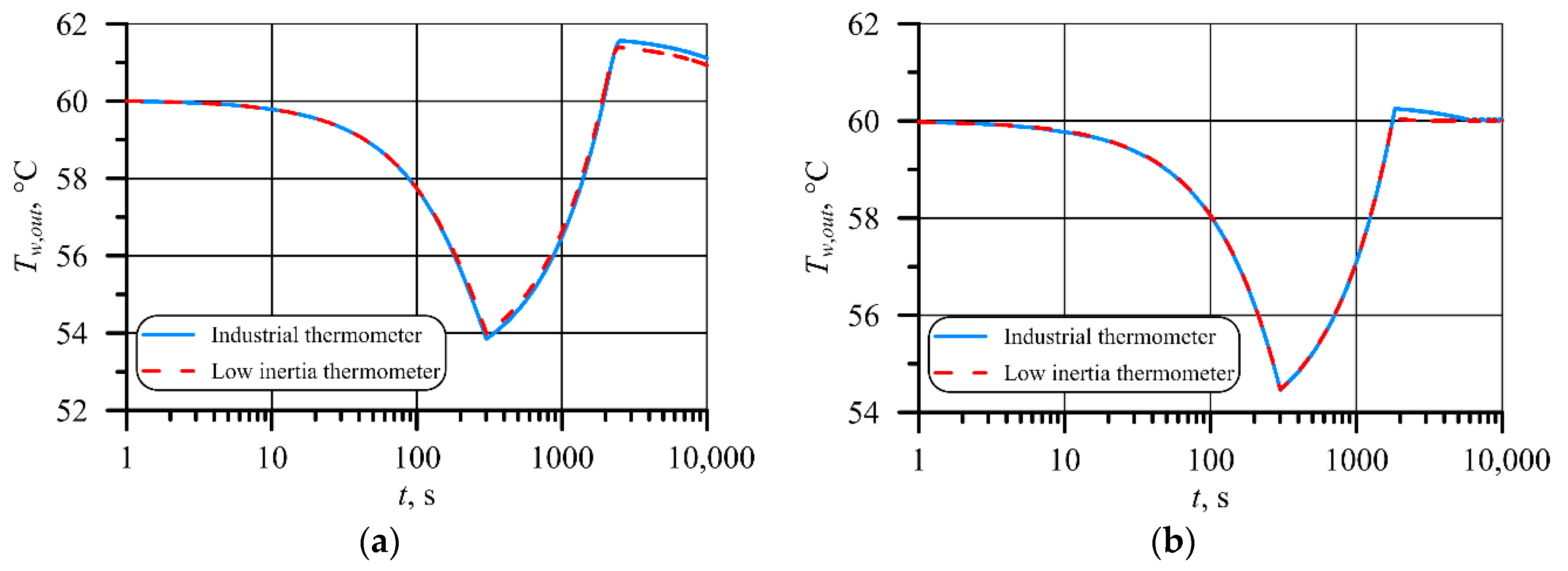
Assuming the value of dynamic temperature measurement error e_Tx = −1% in Equation (23), the required measurement time t_x is obtained, which for an industrial thermometer is 274 s and for a fast-response thermometer 42 s.

It is, therefore, to be expected that the digital PID control system will work faster and more accurately with a fast-response thermometer.

5. Examples of Application of a Digital PID Controller to Maintain a Constant Temperature in the Water Tank

The hot water tank was chosen as a test facility due to, among other things, a simple mathematical model describing transient changes in water temperature. Moreover, in the second-order thermometer model, which is analyzed in the article, it was necessary to determine two time constants experimentally. These constants were determined for hot water for the industrial thermometer and fast response thermometer. The digital PID control system for maintaining the set temperature of water in the tank allowed us to use experimentally verified mathematical models of massive thermometers. A certain disadvantage of the system is its high thermal inertia due to a large amount of water stored in the tank. In such a tank, even thermometers with high thermal inertia work properly. Differences in the quality of water temperature control using a digital PID controller and tested thermometers will be more visible in devices with low thermal inertia, such as, e.g., steam superheaters in power boilers or steam or gas pipelines in which a medium with high temperature and pressure flows.

Two examples of the application of the digital PID controller will be presented. The first example shows a developed control system for changing the volume flow rate of water entering the storage tank. In the second case, the operation of the controller over a long period will be analyzed. The hot water tank has neither been supplied with water nor taken from the storage tank. The electric resistance heater was switched on due to heat losses from water to the environment through the insulated tank wall. For the purpose of the control system, a mathematical model of a volume water heater (heat storage tank) was developed, the diagram of which is shown in Figure 1. The hot water tank was made as a cylindrical tank closed at both ends with elliptical bottoms. The inner diameter of the tank is d_in = 0.445 m, the wall thickness δ_m = 0.0045 m, and the height of the cylindrical part of the tank H_c and the heights of the elliptical head H_eh are 0.818 m and 0.140 m, respectively. The tank is entirely covered with 0.061 m thick thermal insulation made of polyurethane foam with thermal conductivity k_isol = 0.03 W/(m·K). An electric resistance heater with a nominal power of 2500 W was used to heat water in the tank. The temperature of water in the tank was controlled by an industrial thermometer and a fast response thermometer.

5.1. Example I

Water with a temperature of T_w,_in = 15 °C was supplied to the tank, which flowed at a velocity of w_w = 1 m/s. After time t = 300 s the water supply was closed. The changes in water velocity in the feed line is depicted in Figure 8. In the first stage, hot water with a temperature of 60 °C was taken from the tank, and the water loss in the tank was continuously refilled with fresh water with a much lower temperature of 15 °C.

The system of differential Equations (2), (8), and (9) was used to determine the temperature changes of the water and thermometer during the heater operation. The system was solved by the Runge–Kutta method of the fourth order. The power of the electrical heater set by the regulator is depicted in Figure 9. The calculated temperature changes of the thermometers are illustrated in Figure 10, and the water temperature in Figure 11.

Figure 10a and Figure 11a show the temperatures of thermometers and water for the following parameters: the proportional gain of the PID controller K_p = 5.0 W/K, the integral gain K_i = 1 s⁻¹, and the derivative gain K_d = 2 s, which were selected at random without using any algorithm to determine their optimum values. Figure 10b and Figure 11b show industrial and low inertia thermometer temperatures for another set of parameters: K_p = 1640 W/K, the integral gain K_i = 100 s⁻¹, and the derivative gain K_d = 10 s, whose values were determined using trial-and-error tuning. Trial-and-error tuning is well described by Ingham et al. [25] and by Sung et al. [26]. By changing the parameters of the PID controller, the set water temperature is reached faster. After just 1770 s, the water temperature of 60 °C was reached, while in the first case, even after 10,000 s, the water temperature was still unstable. The performance of the PID regulator could be further improved by using more sophisticated PID regulator tuning methods such as the first or second Ziegler–Nichols rules [27], internal model control (IMC) tuning relations, tuning relations based on integral error criteria, or even others [28].

In the case of the fast response thermometer, the heater started to heat at full power of 2500 W after 223 s, and in the case of the industrial thermometer, the time to reach full power of the heater was longer and amounted to 268 s. The control system is more dynamic when using a fast response thermometer. The power of the heater in the adjustment system with the new thermometer starts to decrease after 1908 s, while for the industrial thermometer the time of the beginning of the power reduction was 2001 s.

Better dynamic properties of the fast response thermometer can be seen in Figure 11. When the water temperature drops, the new thermometer shows a lower temperature, both when the water is cooled down during the cold-water supply to the tank and when the electrical power is switched off after 1908 s. It can be seen that if the water temperature is over-regulated above the 60 °C set point, the thermometer temperature drops very slowly. After a time of 1908 s for a new thermometer, the heater is completely switched off, and the drop in the tank water temperature is only caused by heat loss to the environment.

As a result of supplying cold water at a temperature of 15 °C to the tank, the temperature of the water was quickly reduced to around 54 °C (Figure 11). After 300 s, the cold-water supply to the tank has ended.

5.2. Example II

In the second case, it was assumed that no water is taken from the tank. The PID controller settings were as follows: the proportional gain K_p = 5.0 W/K, the integral gain K_i = 1.0 s⁻¹, and the derivative gain K_d = 2.0 s. There is a loss of heat to the environment, which is calculated using Equation (3). The overall heat transfer coefficient of a multi-layer insulated wall U_in given by Equation (4) is related to the internal surface of the tank. Such a situation causes the digital PID controller to switch on the heater as soon as the water temperature decreases slightly and switches off after exceeding the set temperature equal 60 °C. This process is accompanied by the oscillating temperature changes of both types of industrial thermometers (Figure 12) and the water temperature in the tank (Figure 13). As can be seen from Figure 12 and Figure 13, the lower amplitude medium temperature oscillations occur when a modern low inertia thermometer with a smaller time constant is used for temperature measuring.

The range of temperature changes indicated by an industrial thermometer (Figure 12 and Figure 13) is higher than that of a fast response thermometer. Such behavior of thermometers is due to the larger τ₁ and τ₂ time constants for the industrial thermometer compared to the fast response thermometer. The lower amplitudes for both thermometers are identical because the minimum heater power that the regulator can set is 0, i.e., the regulator cannot set the negative power of the heaters.

Although the differences in water temperature oscillations for the fast response and conventional thermometer are marginal, this results in noticeable differences in the electricity used to heat it. Figure 14 illustrates the changes in heater power over time.

Figure 14 illustrates that differences in the power consumed to heat water with a new and conventional thermometer are noticeable. The calculated monthly energy consumption for maintaining a constant tank water temperature was 27.86 kWh when a thermometer with the small time constant was used in the PID control system, and 43.16 kWh when an industrial thermometer was applied. The use of an industrial thermometer with a high time constant will contribute to the increase of electric energy consumption in domestic hot water production.

6. Conclusions

A digital PID control system for maintaining the prescribed temperature in the domestic hot water tank is presented. A conventional thermometer and a special design fast response thermometer were used to measure water temperature. The digital PID system works correctly, even if the initial water temperature is significantly different from the set one. A numerical–mathematical model of the system consisting of a hot water tank and thermometer was developed. The thermometers were modeled as inertial objects of the second order, thanks to which, the delay of thermometer indications could be taken into account. A control system in which a low inertia thermometer is used to measure the water temperature works faster compared to a system in which the water temperature is measured with a conventional thermometer. By using a thermometer with a small time constant, significant savings in hot water preparation costs are achieved. An additional aim of the study was to carry out tests using massive thermometers, which are used to measure the temperature of a liquid under high pressure and flowing at a high velocity. Due to the large heat capacity of the hot water storage tank, the water temperature changes are slow, so there are no significant differences in the operation of the industrial thermometer and the one proposed in this article. In the case of objects with smaller time constants, such as boiler steam superheaters or other heat exchangers, the quality of liquid temperature control at the exchanger outlet with the proposed digital PID controller will be much higher. This is due to the lower thermal inertia of the mentioned heat exchangers.

References

1. Michalski, L.; Eckersdorf, K.; Kucharski, J.; McGhee, J. Temperature Measurement, 2nd ed.; Wiley: Hoboken, NJ, USA, 2001. [Google Scholar]
2. Childs, P. Practical Temperature Measurement; Butterworth-Heinemann: Oxford, UK, 2001. [Google Scholar]
3. McMillan, G.K. Advanced Temperature Measurement and Control, 2nd ed.; International Society of Automation: Research Triangle Park, NC, USA, 2010. [Google Scholar]
4. ASME PTC 19.3 TW-2016 (Revision of ASME PTC 19.3 TW-2010). In Thermowells; An American National Standard; The American Society of Mechanical Engineers: New York, NY, USA, 2016.
5. Jaremkiewicz, M.; Taler, D.; Sobota, T. Measurement of transient fluid temperature. Int. J. Therm. Sci. 2015, 87, 241–250. [Google Scholar] [CrossRef]
6. Jaremkiewicz, M.; Taler, D.; Sobota, T. Measuring transient temperature of the medium in power engineering machines and installations. Appl. Therm. Eng. 2009, 29, 3374–3379. [Google Scholar] [CrossRef] [Green Version]
7. Jaremkiewicz, M. Accurate measurement of unsteady-state fluid temperature. Heat Mass Transf. 2017, 53, 887–897. [Google Scholar] [CrossRef] [Green Version]
8. Jaremkiewicz, M.; Taler, J. Measurement of transient fluid temperature in a pipeline. Heat Transfer Eng. 2018, 39, 1227–1234. [Google Scholar] [CrossRef]
9. Jaremkiewicz, M.; Taler, D.; Dzierwa, P.; Taler, J. Determination of transient fluid temperature and thermal stresses in pressure thick-walled elements using a new design thermometer. Energies 2019, 12, 222. [Google Scholar] [CrossRef] [Green Version]
10. Jaremkiewicz, M.; Dzierwa, P.; Taler, D.; Taler, J. Monitoring of transient thermal stresses in pressure components of steam boilers using an innovative technique for measuring the fluid temperature. Energy 2019, 175, 139–150. [Google Scholar] [CrossRef]
11. Baerts, C.; van Gerwen, P. Method for Decreasing the Response Time of a Temperature Sensor. European Patent EP1069416 (A1), 17 January 2001. [Google Scholar]
12. Dietmann, S.; Wienand, K. Fast response temperature probe especially for measuring temperature in range minus forty to plus one thousand degrees centigrade. German Patent DE4424384 (A1), 18 January 1996. [Google Scholar]
13. Monroe, J.G.; Aspin, Z.S.; Fairley, J.D.; Thompson, S.M. Analysis and comparison of internal and external temperature measurements of a tubular oscillating heat pipe. Exp. Therm. Fluid Sci. 2017, 84, 165–178. [Google Scholar] [CrossRef] [Green Version]
14. Wang, E.; Cheng, P.; Li, J.; Cheng, Q.; Zhou, X.; Jiang, H. High-sensitivity temperature and magnetic sensor based on magnetic fluid and liquid ethanol filled micro-structured optical fiber. Opt. Fiber Technol. 2020, 55, 1–6. [Google Scholar] [CrossRef]
15. Seo, B.; Hwang, H.; Kang, S.; Cha, Y.; Choi, W. Flexible-detachable dual-output sensors of fluid temperature and dynamics based on structural design of thermoelectric materials. Nano Energy 2018, 50, 733–743. [Google Scholar] [CrossRef]
16. Baek, S.; Radebaugh, R.; Bradley, P.E. A new method for heat transfer coefficient measurements of single-phase fluids during laminar flow in microchannels. Int. J. Heat Mass Transf. 2020, 157, 1–11. [Google Scholar] [CrossRef]
17. Rouizi, Y.; Al Hadad, W.; Maillet, D.; Jannot, Y. Experimental assessment of the fluid bulk temperature profile in a mini channel through inversion of external surface temperature measurements. Int. J. Heat Mass Transf. 2015, 83, 522–535. [Google Scholar] [CrossRef]
18. Acosta, C.A.; Yanes, D.; Bhalla, A.; Guo, R.; Finol, E.A.; Frank, J.I. Numerical and experimental study of the glass-transition temperature of a non-Newtonian fluid in a dynamic scraped surface heat exchanger. Int. J. Heat Mass Transf. 2020, 152, 1–8. [Google Scholar] [CrossRef]
19. Castilla, G.M.; Larsson, A.; Lundberg, L.; Johnsson, F.; Pallarès, D. A novel experimental method for determining lateral mixing of solids in fluidized beds—Quantification of the splash-zone contribution. Powder Technol. 2020, 370, 96–103. [Google Scholar] [CrossRef]
20. Burden, R.L.; Faires, J.D.; Burden, A.M. Numerical Analysis, 9th ed.; Brooks Cole Cengage Learning: Boston, MA, USA, 2011; pp. 259–356. [Google Scholar]
21. Gerald, C.F.; Wheatley, P.O. Applied Numerical Analysis, 7th ed.; Pearson: Boston, MA, USA, 2004; pp. 329–404. [Google Scholar]
22. Díaz-Rodríguez, I.D.; Han, H.; Bhattacharyya, S.P. Analytical Design of PID Controllers; Springer International Publishing: Cham, Switzerland, 2019. [Google Scholar]
23. Wang, L. PID Control System Design and Automatic Tuning Using Matlab/Simulink; Wiley: Hoboken, NJ, USA, 2020. [Google Scholar]
24. Press, W.H.; Teukolsky, S.A.; Vetterling, W.T.; Flannery, B.P. Numerical Recipes: The Art of Scientific Computing, 3rd ed.; Cambridge University Press: Cambridge, UK, 2007; pp. 779–839. [Google Scholar]
25. Ingham, J.; Dunn, I.J.; Heinzle, E.; Přenosil, J.E.; Snape, J.B. Chemical Engineering Dynamics: An Introduction to Modelling and Computer Simulation, 3rd ed.; Wiley-VCH Verlag: Weinheim, Germany, 2007; pp. 51–92. [Google Scholar]
26. Sung, S.W.; Lee, J.; Lee, I.-B. Process Identification and PID Control; Wiley: Singapore, 2009; pp. 151–168. [Google Scholar]
27. Ogata, K. System Dynamics, 4th ed.; Pearson Prentice Hall: Upper Saddle River, NJ, USA, 2004; pp. 566–607. [Google Scholar]
28. Seborg, D.E.; Edgar, T.F.; Mellichamp, D.A.; Doyle, F.J., III. Process Dynamics and Control, 3rd ed.; Wiley: Hoboken, NJ, USA, 2011; pp. 217–232. [Google Scholar]
Figure 1. Hot water storage tank; Heh—the height of tank elliptical head, Hc—the height of cylindrical part of the container, Hiso—the height of tank thermal insulation, dout—outer diameter of the water storage tank, disol—outer diameter of thermal insulation, Vw—tank capacity, V ˙ s t r —water volume flow rate, m3/s.
Energies 13 04039 g001
Figure 2. The thermal circuit for heat flow from hot water through a metal tank wall and thermal insulation to the environment; q ˙ i n , q ˙ o u t —heat flux ant the inner surface of the tank wall and outer surface of the insulation, Tw,out—water temperature at the tank, Twall,in, Twall,out—the temperature of the inner and outer surface of the tank wall, Tisol,out—the temperature of the outer surface of the insulation, Tenv—environment temperature.
Energies 13 04039 g002
Figure 3. Block diagram of PID control system to maintain constant hot water temperature in the tank; T w , o u t s e t —the set temperature of the water in the tank, Tw,out—the temperature of the water in the tank and its outlet, Tt—thermometer temperature, Q ˙ e l —the power of the electric heater, D(t)—disturbances, e—the difference between the preset and actual measured value.
Energies 13 04039 g003
Figure 4. Thermometers used to measure the water temperature: (a) classic industrial thermometer, (b) innovative in-house design of the thermometer with small times constant.
Energies 13 04039 g004
Figure 5. Stepwise increase in the temperature of the fluid (a) and the thermometer transient response (b).
Energies 13 04039 g005
Figure 6. The time response of the industrial thermometer; (a) linear time coordinate, (b) logarithmic time coordinate.
Energies 13 04039 g006
Figure 7. The time response of the fast-response thermometer; (a) linear time coordinate, (b) logarithmic time coordinate.
Energies 13 04039 g007
Figure 8. Water velocity in the tank feed tube.
Energies 13 04039 g008
Figure 9. Electric power of the heater as a function of time.
Energies 13 04039 g009
Figure 10. Temperature variations of the industrial thermometer and fast response thermometer obtained for the following PID controller settings: (a) Kp = 5.0 W/K, the integral gain Ki = 1 s−1, and the derivative gain Kd = 2 s, (b) Kp = 1640 W/K, the integral gain Ki = 100 s−1, and the derivative gain Kd = 10 s.
Energies 13 04039 g010
Figure 11. Changes in water temperature in the water volume heater obtained for the following PID controller settings: (a) Kp = 5.0 W/K, the integral gain Ki = 1 s−1, and the derivative gain Kd = 2 s, (b) Kp = 1640 W/K, the integral gain Ki = 100 s−1, and the derivative gain Kd = 10 s.
Energies 13 04039 g011
Figure 12. Temperature variations of the low inertia and industrial thermometer as a function of time.
Energies 13 04039 g012
Figure 13. Temperature variations of the water temperature for low inertia and industrial thermometer as a function of time.
Energies 13 04039 g013
Figure 14. Electric heater power oscillations during PID control process.
Energies 13 04039 g014