Experimental Calibration and Validation of a Simulation Model for Fault Detection of HVAC Systems and Application to a Case Study

Abstract

Automated fault detection and diagnostics (FDD) could provide a cornerstone for predictive maintenance of heating, ventilation and air-conditioning (HVAC) systems based on the development of simulation models able to accurately compare the faulty operation with respect to nominal conditions. In this paper, several experiments have been carried out for assessing the performance of the HVAC unit (nominal cooling/heating capacity of 5.0/5.0 kW) controlling the thermo-hygrometric comfort inside a 4.0 × 4.0 × 3.6 m test room at the Department of Architecture and Industrial Design of the University of Campania Luigi Vanvitelli (Italy); then, a detailed dynamic simulation model has been developed and validated by contrasting the predictions with the measured data. The model has also been used to analyze the dynamic variations of key parameters associated to faulty operation in comparison to normal performance, in order to identify simplified rules for detection of any non-optimal states of HVAC devices. Finally, the simulated performance of the HVAC unit has also been investigated while serving a typical Italian building office with and without the occurrence of typical faults with the main aim of assessing the impact of the faults on thermo-hygrometric comfort conditions as well as electric energy consumption.

1. Introduction

HVAC (heating, ventilation and air-conditioning) systems including air-handling units (AHUs) for space heating, space cooling and ventilation of buildings represent one of the most significant sources of the world’s energy demand [1,2]. In more detail, the residential and tertiary sectors are responsible for nearly 40% of energy use [3] and globally implemented energy efficiency measures in the building sector could deliver CO₂ emissions savings as high as 5.8 billion tons by 2050 [3].

Due to lack of proper maintenance, failure of components or incorrect installation, HVAC units are frequently run in faulty conditions where a fault is intended as an unpermitted deviation of at least one characteristic property of the system from the acceptable, usual, standard condition; a study conducted on more than 55,000 HVAC systems, showed that 90% of them runs with one or multiple faults [4]. Faults could result in inefficient usage of energy and/or uncomfortable environment, unless corrective action is taken. Yu et al. [5] highlighted that (i) typical faults of HVAC units are responsible for 25–50% of energy waste in buildings located in the United Kingdom and (ii) this inefficiency could be strongly decreased below 15% thanks to early detection and identification of faulty operation [5]. Yan et al. [6] estimated that the identification and diagnosis of faults in HVAC units can lead to potential savings of about 30%.

Companies follow different maintenance programs in order to guarantee the reliability of systems and reduce the costs; generally, a reactive or a preventive maintenance is adopted. In the case of reactive maintenance, a system is used up to its limits and the repairs are performed only after the system failure; this kind of approach is not convenient with reference to complex systems mainly due to the fact that repairing the damaged parts after failure could (i) be extremely expensive and (ii) cause safety issues. For this reason, it could be useful to prevent the failures by performing regular checks on the equipment by means of preventive maintenance; in this case, the systems are inspected and maintained at fixed time intervals, independent of their actual condition. However, one of the main challenges of this approach is to determine when the maintenance has to be performed; it has to be conservative in order to prevent safety issues as well as reduce the costs of failures, but scheduling the maintenance very early could mean wasting system life that is still usable. The aforementioned critical points associated to both reactive and preventive maintenance programs highlight how “predicting” the failures of components could be extremely important in minimizing the related costs, optimizing the performance as well as avoiding safety issues.

Fault detection and diagnosis (FDD) [5,7,8,9,10] methods can monitor the operation of HVAC components as well as detect and predict the presence of the defects (deviations from normal or expected operation) causing a faulty operation. Ideally, FDD systems could also resolve (diagnose) the type of problem and/or identify its location, giving instructions for undertaking corrective actions. Efficient FDD methods could detect faults before the building occupants notice the effects and they would reduce the repair and maintenance costs of the plants. In addition, these tools could provide manufacturers with information about the design and sales of devices with the aim of identifying where enhancements are required. Moreover, improving the operation of HVAC systems could significantly reduce energy consumption and related emissions. Finally, integrating FDD systems into modern HVAC plants could improve the system efficiency as well as the indoor thermo-hygrometric conditions.

FDD methods are based on the use of accurate instruments measuring key parameters, the variation of which in comparison to a “nominal/healthy” trend is assumed as a symptom of defects; once the test quantity reaches some predetermined levels that reflect the seriousness of the defect requiring corrective actions to take place, the test quantity is set into an alarm state (symptom) and reasoning is started to find the cause of the “alarm-symptom–fault” chain [10,11,12]. In order to apply FDD methods to HVAC units or components, it is necessary to compare real behavior of the systems to the “nominal/healthy” operation without faults that can be modeled by means of a simulation software and/or artificial intelligence techniques. Simulation tools represent a useful approach not only in the design phase, but also in combination with FFD methods thanks to the fact that they could have the required accuracy to predict thermal/cooling loads, energy consumption and quality of indoor environment of buildings, thus allowing for the detection of any non-optimal states of performance by comparing the simulation results with the normal data.

One of the main disadvantages of the FDD approach is that it could require a continuous monitoring with specifically devoted instrumentation and, therefore, the aforementioned benefits alone could fail in justifying the cost of implementing FDD methods [5,12]. As a consequence, in order to obtain a wider utilization of FDD systems, the benefits of this approach throughout the value chain have to be assessed in greater detail. Moreover, the extra investment cost associated with the application of FDD systems should be shared by different parties (electric-grid operators, manufacturers, dealers, installers, service companies, customers) and economic incentives should be put in place to support and speed up their diffusion [5,12]. The prediction of faulty operation is also problematic since some types of faults cannot be easily and practically introduced, and the artificial implementation of faulty conditions may enhance the energy costs or the discomfort of occupants in the built environment; an additional issue is represented by the fact that a strong anomaly detection capability is significantly dependent on the accuracy of measurement sensors. Finally, it should be underlined that a robust data analytics-based FDD tool should be able to automatically prevent the generation of false alarms (for example due to high uncertainty of the instrumentation) that could negatively affect the methods [5,12]. Therefore, additional studies have to be carried out in order to better highlight and evaluate the potential applications and benefits/drawbacks associated with FDD techniques.

FDD techniques have been used for many years in aerospace, nuclear and industrial sectors, and their use in building operation and control applications is becoming more widespread [5,13,14,15,16,17,18]. Several methods and procedures aiming at optimizing the application of FDD tools have been developed in the Annex 25 of the International Energy Agency’s (IEA) Energy Conservation in Buildings and Community System (ECBCS) [13] and then applied to existing buildings in the IEA ECBCS Annex 34 [14]. Furthermore, since 2010 studies on FDD systems steadily increased. Several reviews of FDD studies focusing on AHUs are already available in the literature [5,15,16,17,18]. The literature review demonstrated that a number of recent studies have made significant contributions to the advancement of FDD methods in the building sector, how active the FDD research field is, as well as the high contribution that data analytics methodologies bring. However, the outcomes of these reviews highlight that the application of FDD methods is still in its early stage and there are significant research gaps to be further investigated. In particular, Kim and Katipamula [16] highlighted that:

• much more research is needed with reference to the identification of threshold values to be used for the detection of faults in the rule-based FDD techniques in order to avoid the generation of false alarms or the mis-identification of faults;
• the estimation of severity of faults and their energy impact has been poorly assessed; therefore, building operators lack the knowledge to decide whether or not to address and/or repair the faults;
• additional investigations should be performed with the aim of adapting the FDD methods to the variations in the configuration of HVAC units.

In addition, Katipamula and Brambley [17,18] indicated that the following points require additional attention:

• a few papers have been published to date on prognostics for HVAC systems; therefore, a significant lack of information based on which decisions can be made regarding the transition from reactive/preventive maintenance as practiced today to future applications of predictive maintenance is recognized;
• there is a need to more clearly assess the potential drawbacks and benefits associated to FDD applications, identify benchmarks for acceptable costs and provide market information about FDD methods in order to better demonstrate the value of these technologies;
• additional research is needed in order to further develop the selection and specialization of FDD methods to the constraints of the built environment as well as a more extensive testing of FDD methods to different systems and components adopted in buildings.

An innovative multi-sensorial laboratory, called the SENS-i Lab, has been set-up at the Department of Architecture and Industrial Design of the University of Campania Luigi Vanvitelli (Italy). The laboratory is equipped with an AHU (nominal cooling/heating capacity of 5.0/5.0 kW) aiming to control the thermo-hygrometric comfort inside a 4.0 × 4.0 × 3.6 m test room; the AHU is fully instrumented in order to monitor and control its operation. In this paper, several experiments have been carried out for assessing the performance of the AHU upon varying the boundary conditions; then, a detailed dynamic simulation model has been developed by means of the software TRNSYS [19] and validated by contrasting the predictions with the measured data. Then, the model has been used to analyze and investigate the dynamic variations of key parameters associated to faulty operations in comparison to “normal” performance, in order to identify simplified rules for detection of any non-optimal states of AHU. Finally, the performance of the AHU has also been investigated while serving a typical Italian building office with and without the occurrence of typical faults of AHUs with the main aim of assessing the impact of faults on comfort conditions as well as electric energy consumption. This study aims at covering some of the most important research gaps in the FDD research field and its main objectives can be summarized as follows: (i) suggest threshold values or simplified rules to identify typical HVAC faults in order to avoid the generation of false alarms or the mis-identification of faults; (ii) assess the potential drawbacks and benefits associated to FDD applications in order to better identify the value for these technologies; (iii) estimate the severity of typical faults and their energy impacts in order to help the building operators in understanding whether or not to address and/or repair the faults.

2. Description of the Laboratory and Heating, Ventilation and Air-Conditioning (HVAC) System

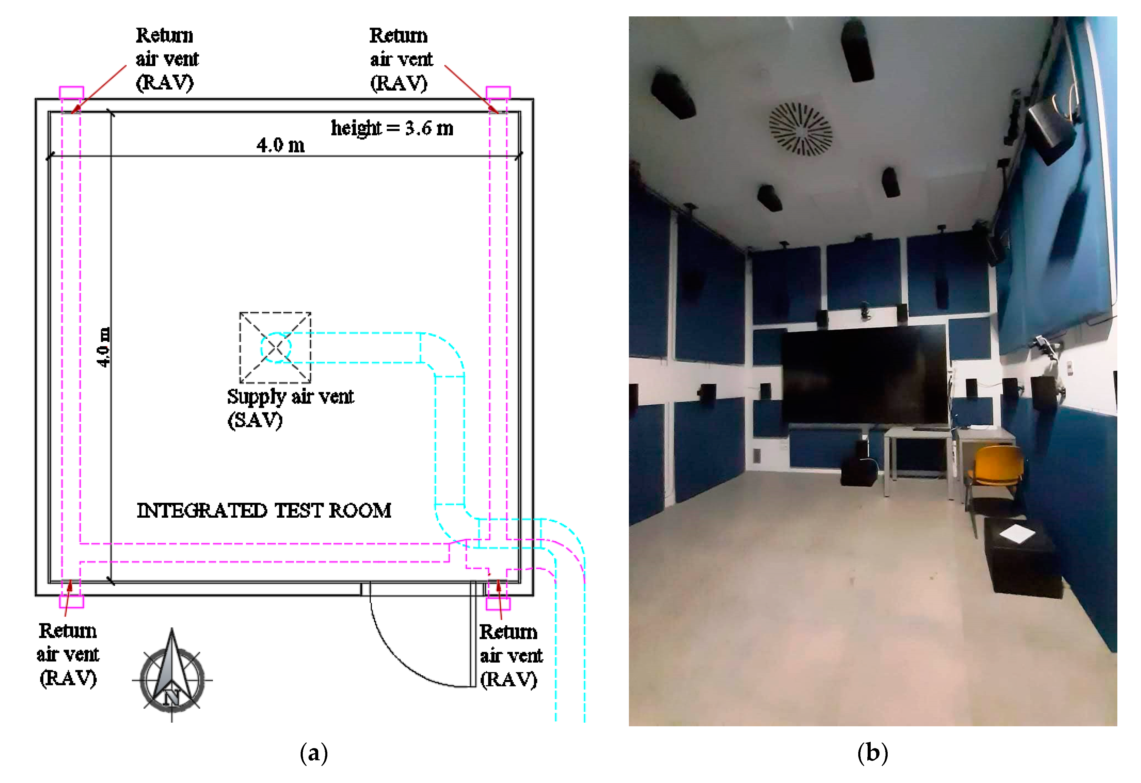
The SENS i-Lab is an innovative, multi-sensorial and multi-purpose laboratory, located at the Department of Architecture and Industrial Design of the University of Campania Luigi Vanvitelli (Aversa, Italy, latitude: 40°58′21″ N, longitude: 14°12′26″ E). The laboratory consists of an Integrated Test Room, allowing in vivo or in virtual, subjective tests to be carried out where the human experience of urban/rural or industrial environments, architectures and products, can be measured. The lab is served by an HVAC system including an air-handling unit able to control the indoor air temperature, relative humidity, velocity and quality inside the Integrated Test Room The room is characterized by a floor area of 16.0 m² with a height of 3.6 m; it is composed of four internal vertical walls, a horizontal ceiling as well as a horizontal floor; two of the vertical walls as well as the floor are integrated with radiant panels for heating/cooling purposes; a door is installed on the south-oriented wall. It is located inside a large open space of the department, so that it is not directly affected by the external climatic conditions. Figure 1 depicts the floor plan of the Integrated Test Room together with an internal view, while

Table 1. Test room envelope characteristics of the Integrated Test Room.

Element of Test Room Envelope	Layer Material (from Outside to Inside)	Thickness (m)	Thermal Conductivity (W/mK)	Conductive Thermal Resistance (m2K/W)		Area (m2)
Horizontal ceiling	Plasterboard	0.0125	0.250	0.050	2.023	16.00
	Rock wool	0.0800	0.042	1.905
	Polyurethane panel	0.0150	0.220	0.068
Horizontal floor	Subfloor	0.1000	1.350	0.074	3.107	16.00
	Tiles	0.0500	2.100	0.024
	Polystyrene panel	0.0800	0.035	2.286
	Galvanized steel slab	0.0020	52.000	0.000
	Tiles	0.0100	1.050	0.010
Vertical walls with radiant panels (West and East oriented)	Plasterboard	0.0125	0.250	0.050	2.005	14.40
	Rock wool	0.0800	0.042	1.905
Vertical walls without radiant panels (South and North oriented)	Plasterboard	0.0125	0.250	0.050	1.998	14.4
	Rock wool	0.0800	0.042	1.905
	Fibre-cement panel	0.0150	0.350	0.043
Door (South oriented)	Soft wood	0.0500	0.140	0.357	0.357	1.68

describes the number and characteristics of layers composing the envelope of the Integrated Test Room.

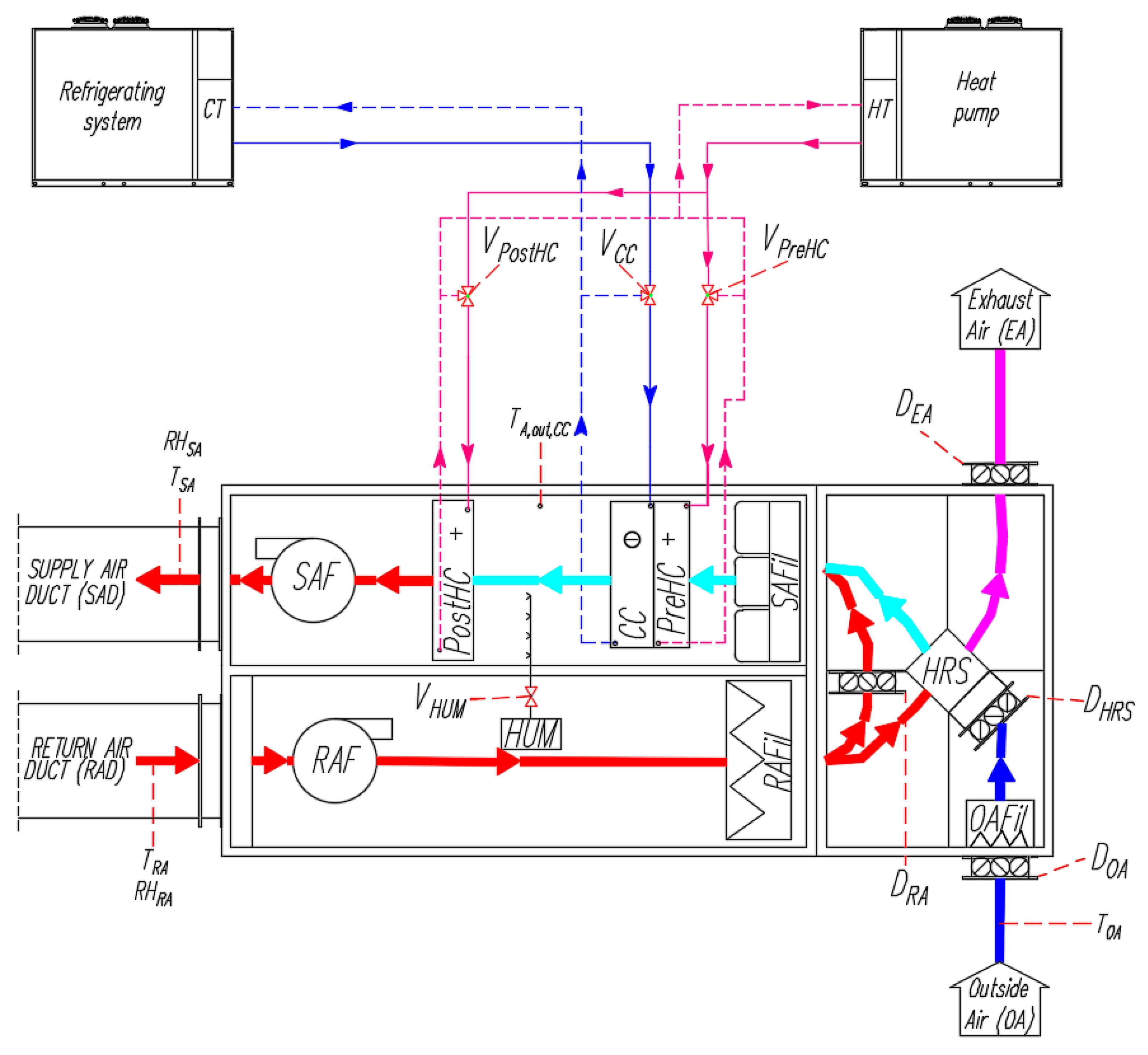
Figure 2 reports the schematic of the AHU serving the Integrated Test Room.

The AHU is composed of the following main components: supply air fan (SAF), return air fan (RAF), pre-heating coil (PreHC), cooling coil (CC), steam humidifier (HUM), post-heating coil (PostHC), cross flow static heat recovery system (HRS), single-stage vapor-compression air-to-water electric refrigerating unit (supplying the CC), single-stage vapor-compression air-to-water electric heat pump (supplying both the PreHC and PostHC), valves (V_PreHC, V_PostHC, V_CC, V_HUM) regulating the heat carrier fluid flow rate entering, respectively, the PreHC, PostHC, CC and HUM, outside air damper (D_OA), return air damper (D_RA), exhaust air damper (D_EA), damper of heat recovery system (D_HRS), outside air filter (OAFil), return air filter (RAFil), supply air filter (SAFil). Two 0.08 × 0.18 cm return air intake vents (RAV) are installed on the south-oriented wall and two 0.08x0.18 cm return air intake vents are installed on the north-oriented wall in order to extract air from the indoor space to be returned to the air-handling unit; a 0.60 × 0.60 cm square ceiling swirl diffuser is installed on the ceiling of the room and used as a supply air vent (SAV).

Table 2. Characteristics of main AHU components.

Supply (SAF)/Return (RAF) air fan	Type	Backward blades
	Nominal power of supply/return air fan	2.50/0.50
	Nominal supply/return air flow rate (m3/h)	600/600
	Nominal revolutions per minute of supply/return air fan (rpm)	2754/2221
	Maximum revolutions per minute of supply/return air fan (rpm)	3640/3080
Cross flow static heat recovery system (HRS)	Efficiency (%)/Recovery capacity (kW)	74.7/3.1
	Pressure drop on the external/exhaust air side (kPa)	0.047/0.048
Return (RAFil) and outside (OAFil) air filter	Filter type/Efficiency class	Fluted/G4
Supply air filter (SAFil)	Filter type/Efficiency class	Rigid pocket/G4
Return (RAD) and supply (SAD) air ducts	Diameter (m)	0.25
	Supply/Return length (m)	9.8/16.8
	Thermal resistance of the insulating material (m2K/W)	0.25
Supply air vent (SAV)	Nominal size (m)	0.60 × 0.60
	Maximum volume flow rate (m3/h)	1080
Pre-heating coil (PreHC)	Nominal heating capacity (kW)	4.1
	Nominal heat carrier fluid/air flow rate (m3/h)	0.710/600
	Nominal heat carrier fluid/air pressure drop (kPa)	12.43/0.00321
Cooling coil (CC)	Nominal cooling capacity (kW)	5.0
	Nominal heat carrier fluid/air flow rate (m3/h)	0.860/600
	Nominal heat carrier fluid/air pressure drop (kPa)	13.56/0.0178
Humidifier (HUM)	Steam capacity (kg/h)/Nominal power (kW)	5.0/3.7
Post-heating coil (PreHC)	Nominal heating capacity (kW)	5.0
	Nominal heat carrier fluid/air flow rate (m3/h)	0.860/600
	Nominal heat carrier fluid/air pressure drop (kPa)	20.35/0.0497
Vapor compression electric Heat Pump (HP)/Refrigerating System (RS) [20]	Nominal heating/cooling capacity (kW)	14.0/13.4
	Nominal input power (kW)	4.75/4.48
	Nominal fluid flow rate (m3/h)	2.41/2.31

describes the main characteristics of the main AHU components. The heat carrier fluid is a mixture of water and ethylene glycol (90/10% by volume). The hot heat carrier fluid supplying both the pre-heating coil as well as the post-heating coil is obtained thanks to the operation of the heat pump, while the refrigerating system is used to provide the cold heat carrier fluid flowing inside the cooling coil. The model ANL 050HQ [20] is used as a vapor compression electric heat pump (HP), while the model ANL 050Q [20] is adopted as a refrigerating system (RS). A 75 L cold thermal energy tank (CT) as well as a 75 L hot thermal energy storage (HT) are coupled with the refrigerating unit and the heat pump, respectively, in order to store the thermal/cooling energy of the heat carrier fluid.

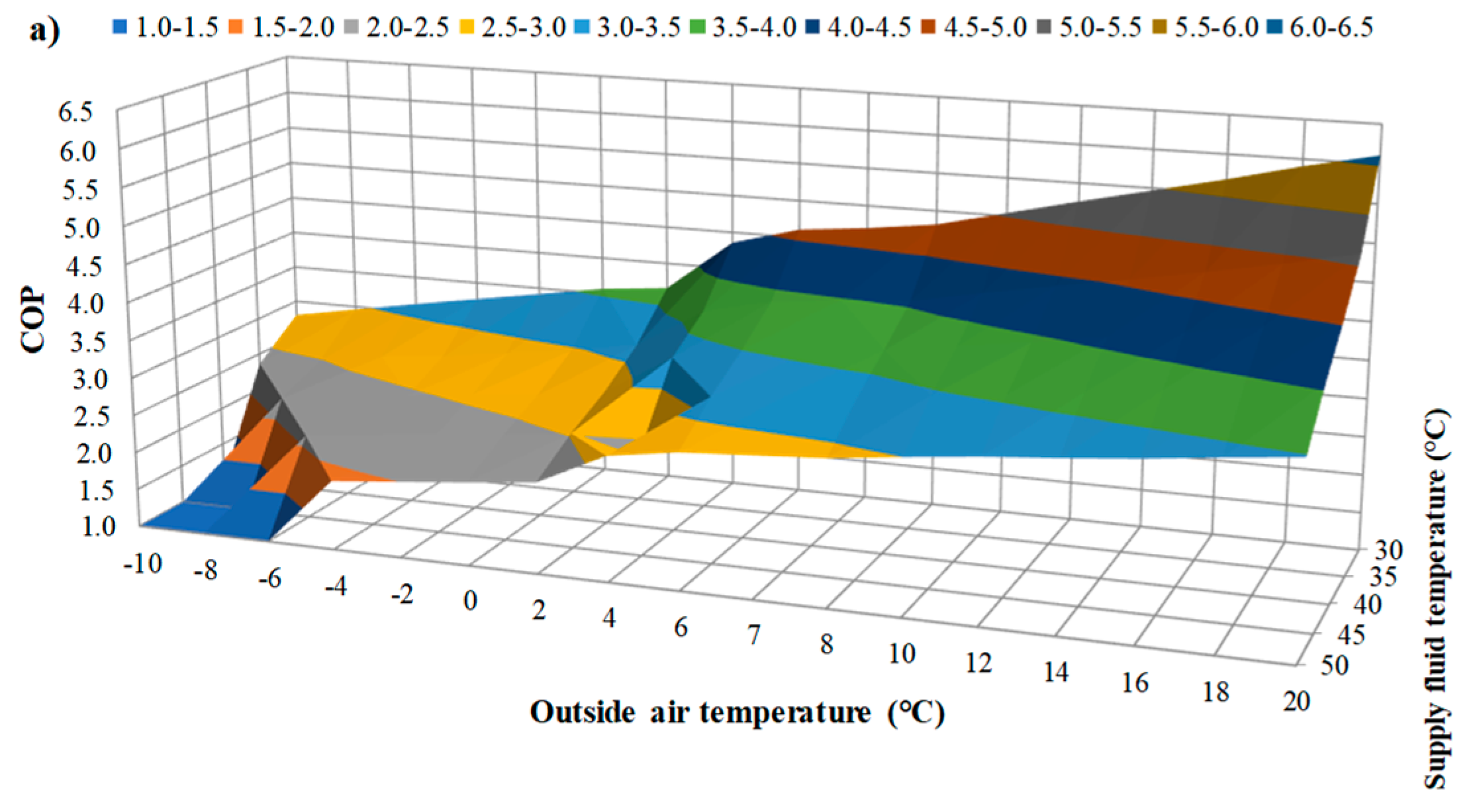
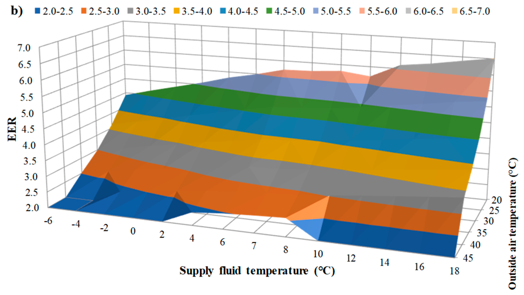
The coefficient of performance (COP, i.e., the ratio between thermal output and power input) of the air-to-water vapor compression heat pumps as well as the energy efficiency ratio (EER, i.e., the ratio between cooling output and power input) of the air-to-water vapor compression refrigerating systems strongly depend on the outside air temperature as well as the supply temperature of the heat carrier fluid. In particular, given the outside temperature, the COP of the heat pumps decreases upon increasing the supply temperature of the heat carrier fluid; on the other hand, given the supply temperature of the heat carrier fluid, the COP of the heat pumps increases at increasing the outside air temperature. The EER of the refrigeration units increases upon increasing the supply temperature of the heat carrier fluid for a given outside air temperature; on the other hand, the EER of the refrigeration units decreases upon increasing the outside air temperature for a given supply temperature of the heat carrier fluid. Figure 3a,b indicate the values of COP and EER (provided by the manufacturer [20]) of the heat pump (model ANL 050HQ [20]) and the refrigeration system (model ANL 050Q [20]), respectively, used in this study as a function of both outside air temperature and supply fluid temperature. In particular, a supply fluid temperature between 30 °C and 50 °C together with an outside air temperature in the range −10–20 °C are considered for the HP; a supply fluid temperature between 20 °C and 45 °C together with an outside air temperature in the range −6–18 °C are considered for the RS. According to the manufacturer’s data [20], the COP of the heat pump varies between 1.91 and 6.11, while the EER of the RS is in the range 2.40–6.52; in greater detail, the COP of the heat pump investigated in this paper ranges between 2.11 and 4.06 for a supply fluid temperature of 45 °C, while the EER of the refrigerating system considered in this study is in the range 2.53–5.73 for a supply fluid temperature of 7 °C.

The AHU is fully equipped in order to monitor, control and record the main operating parameters of the system. The main characteristics of the sensors are reported in

Table 3. Characteristics of the sensors used for the AHU monitoring.

Model	Monitored Parameter	Measuring Range	Accuracy
Siemens QFM2160 [21]	Return air temperature TRA	0–50 °C	±0.8 K
	Return air relative humidity RHRA	0–100%	±3%
Siemens QFM2160 [21]	Supply air temperature TSA	0–50 °C	±0.8 K
	Supply air relative humidity RHSA	0–100%	±3%
Siemens QAM2161.040 [22]	External air temperature TOA	−50–50 °C	±0.75 K
Siemens QAM2161.040 [22]	Air temperature TA,out,CC at outlet of the CC	−50–50 °C	±0.75 K
TSI 7575, 982 IAQ [23]	Air temperature around the room TBEA	−10–60 °C	±0.50 K
	Air relative humidity around the room RHBEA	5–95%	±3%

.

The end-users can manually set: the desired targets of both the indoor air temperature (T_SP,Room) and relative humidity (RH_SP,Room) to be achieved inside the test room, the deadbands DB_T and DB_RH for both T_SP,Room and RH_SP,Room, respectively, the velocity of both the return air fan (OL_RAF) and the supply air fan (OL_SAF), the opening percentages of the return air damper (OP_DRA), the outside air damper (OP_DOA), the exhaust air damper (OP_DEA) and the static heat-recovery system damper (OP_DHRS). The air flow rate moved by the supply air fan can be varied between 0 (OL_SAF = 0%) and 4800 m³/h (OL_SAF = 100%), while the air flow rate of the return air fan is in the range from 0 (OL_RAF = 0%) to 2050 m³/h (OL_RAF = 100%). The parameters OP_DRA, OP_DOA and OP_DEA can be varied in the range 0–100%, where 100% means that the dampers are fully open. The parameter OP_DHRS can be set to 100% (the heat recovery does not occur) or 0% (the heat recovery from return air flow takes place).

A specific control logic has been developed by the manufacturer in order to control the operation of the system and achieve the desired targets.

Table 4. Control strategies of the AHU.

Component of the AHU	ON	OFF
Humidifier (HUM)	RHRA ≤ (RHSP,Room − DBRH)	RHRA ≥ (RHSP,Room + DBRH)
Cooling coil (CC)	TRA ≥ (TSP,Room + DBT) OR RHRA ≥ (RHSP,Room + DBRH)	TRA ≤ (TSP,Room − DBT) AND RHRA ≤ (RHSP,Room − DBRH)
Post-heating coil (PostHC)	TRA ≤ (TSP,Room − DBT)	TRA ≥ (TSP,Room + DBT)
Vapor compression electric Heat Pump (HP)–model ANL 050HQ [20]	THT < (45 °C − 1 °C)	THT ≥ (45 °C + 1 °C)
Refrigerating System (RS)–model ANL 050Q [20]	TCT > (7 °C + 1 °C)	TCT ≤ (7 °C − 1 °C)

describes the conditions controlling the activation and deactivation of the main components of the AHU. Even if the AHU is equipped with a PreHC, this component is never used during normal operation (always de-activated).

The heating coil is devoted to controlling the temperature inside the test room; therefore, its operation is based on the difference between the target temperature inside the test room T_SP,Room (set by the end-users) and the current temperature of return air T_RA, with a given deadband DB_T.

The cooling coil is devoted to satisfying the requirements in terms of both temperature and relative humidity inside the test room; as a consequence, its activation depends on both the difference between target (T_SP,Room) and current (T_RA) temperatures of return air (with a given deadband DB_T) as well as the difference between target (RH_SP,Room) and current (RH_RA) relative humidity of return air (with a given deadband DB_RH).

The humidifier is devoted to enhancing the relative humidity inside the test room; its operation is based on the difference between the target of relative humidity RH_SP,Room inside the test room set by the end-users and the current relative humidity of return air RH_RA, with a given deadband DB_RH.

The operation of the humidifier as well as the flow rate of the heat carrier fluid entering the post-heating coil or the cooling coil can be continuously adjusted between 0% and 100% depending on the differences between the target and current values of parameters to be controlled. In particular, the heat carrier fluid flow rate flowing into the cooling coil or the post-heating coil can ben varied between 0 (OP_{V_CC}/OP_{V_PostHC} = 0%) and 0.860 m³/h (OP_{V_CC}/OP_{V_PostHC} = 100%), while the steam mass flow rate can be modulated from 0 (OP_{V_HUM} = 0%) up to 5 kg/h (OP_{V_HUM} = 100%).

The operation of both the refrigerating unit and the heat pump is controlled in order to maintain the desired temperatures inside the related tanks; in particular, the refrigeration device operates in order to maintain a temperature T_CT of 7 °C (with a deadband of 1 °C) inside the cold tank, while the heat pump is activated with the aim of achieving a temperature T_HT of 45 °C (with a deadband of 1 °C) inside the hot tank.

3. Experimental Tests

Firstly, the air velocity or volumetric flow rate of supply air, return air, outside air and exhaust air) in front of the air vents have been measured upon varying the operating conditions. The results of measurements are reported in

Table 5. Boundary conditions during the measurements of air velocity or volumetric flow rate.

OPSAF (%)	OPRAF (%)	OPDRA (%)	OPDOA (%)	OPDEA (%)	OPDHRS (%)	Supply Air Flow Rate (m3/h)	Return Air Velocity (m/s)	Outside Air Velocity (m/s)	Exhaust Air Velocity (m/s)
50	50	100	20	20	100	430	4.4	1.6	3.3
90	50	100	20	20	100	980	4.8	3.8	1.5
70	50	100	20	20	100	680	4.7	2.1	3.2
30	50	100	20	20	100	206	4.3	1.3	4.6
10	50	100	20	20	100	85	4.0	1.2	4.8
50	90	100	20	20	100	470	7.5	1.8	7.5
50	70	100	20	20	100	450	5.6	1.4	7.2
50	30	100	20	20	100	420	2.5	1.8	1.3
50	10	100	20	20	100	400	0.9	1.2	1.2
50	50	80	20	20	100	436	4.5	0.8	4.0
50	50	60	20	20	100	456	4.5	0.9	4.1
50	50	40	20	20	100	450	4.3	0.9	5.0
50	50	20	20	20	100	418	3.9	1.2	6.6
50	50	100	40	20	100	447	4.2	0.9	4.0
50	50	100	60	20	100	450	4.3	0.9	3.9
50	50	100	80	20	100	455	4.2	1.0	4.0
50	50	100	100	20	100	462	4.3	1.2	3.9
50	50	100	20	40	100	457	4.4	1.3	0.6
50	50	100	20	60	100	461	4.3	1.4	0.6
50	50	100	20	80	100	465	4.3	0.9	0.6
50	50	100	20	100	100	464	4.3	0.8	0.6
50	50	100	20	20	0	462	4.4	0.9	3.7

as a function of OP_SAF, OP_RAF, OP_DRA, OP_DOA, OP_DEA OP_DHRS. The air volumetric flow rate measurements have been performed by using the TSI ProHood Air Capture Hood model PH731 [24], characterized by a measuring range from 42 to 4250 m³/h together with an accuracy ±12 m³/h, whereas the air velocity measurements have been performed by using the hot wire anemometer KIMO AMI 301 [25], characterized by a measuring range from 0 to 30 m/s together with an accuracy of ±3% of readings.

Four experiments have been carried out to investigate the HVAC behavior during steady-state and transient operations.

Table 6. Boundary conditions of experimental tests.

Test Number	1	2	3	4	5	6	7
TSP,Room (°C)	22 → 24 → 26	26 → 24 → 22	22	28	22	22	22
TRoom_initial (°C)	19.8	28.1	22.0	28.1	23.1	23.0	23.1
RHSP,Room (%)	50.0	50.0	60 → 70	55 → 45	50	50	50
RHRoom_initial (%)	52.5	51.1	51.4	64.8	61.2	50.6	53.5
OLRAF (%)	50	50	50	50	50	50	100
OLSAF (%)	50	50	50	50	50	50	100
DRA (%)	100	100	100	100	0	50	100
DOA (%)	20	20	20	20	100	50	20
DEA (%)	20	20	20	20	100	50	20
Duration (h)	6.82	5.97	0.70	0.95	1.23	1.00	0.52

describes the operating conditions of the tests in terms of target indoor air temperature T_SP,Room, target indoor air relative humidity RH_SP,Room, initial indoor air temperature T_{Room_initial} and indoor relative humidity RH_{Room_initial} in the test room, OL_RAF, OL_SAF, D_RA, D_OA, D_EA and duration. The experiments were carried out by measuring the parameters indicated in Table 3 every minute and maintaining constant the following conditions: DB_T = 1 °C, DB_RH = 5%, and OP_DHRS = 100%. During all tests the following parameters have been maintained constant: OL_RAF = 50% and OL_SAF = 50%; during the tests n. 1, 2, 3 and 4 the following parameters have been maintained constant: OP_DRA = 100%, OP_DOA = 20% and OP_DEA = 20%; during the tests n. 5 and 6 the opening percentages of the return air damper, the outside air damper and the exhaust air damper have been modified with respect to the tests n. 1, 2, 3 and 4.

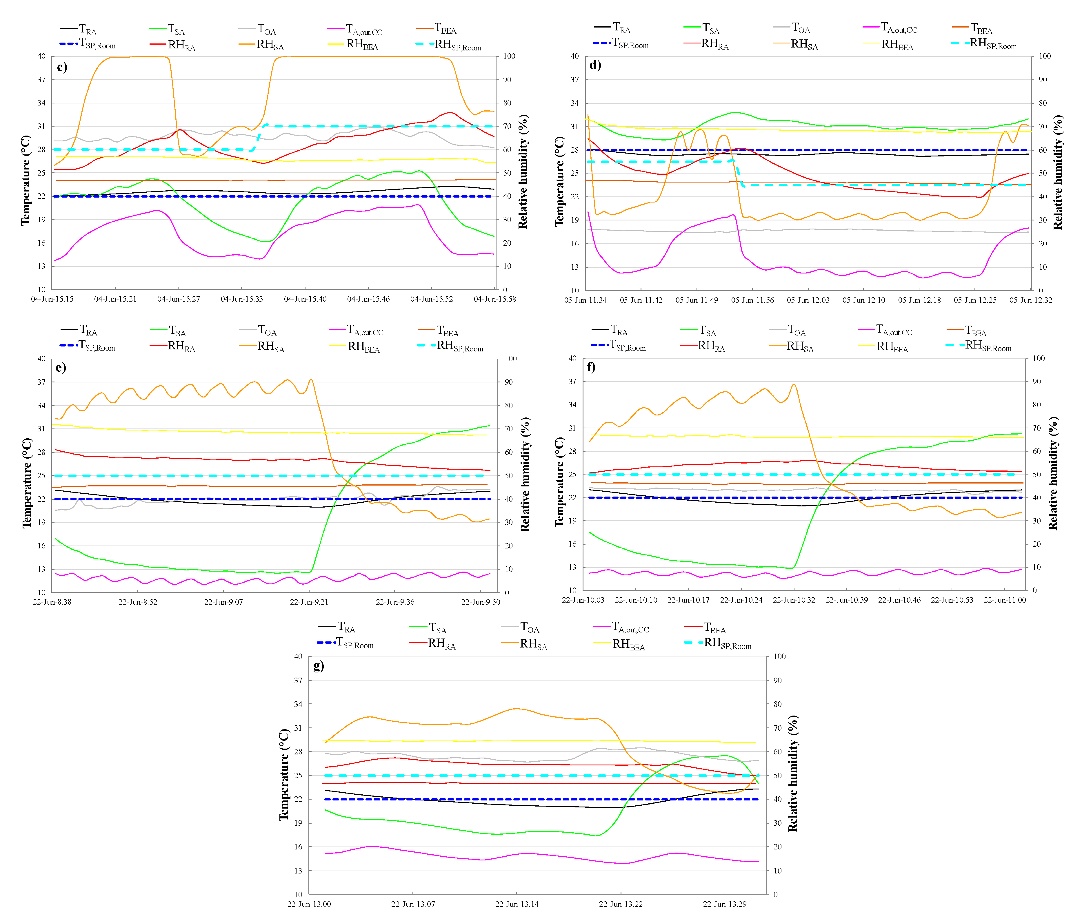
During the test n.1 the target for indoor air relative humidity is fixed at 50%, while the target for indoor air temperature is gradually increased from 22 °C up to 26 °C; during the test n. 2 the target for indoor air relative humidity is maintained at 50%, while the target for indoor air temperature is gradually reduced from 26 °C up to 22 °C; during the test n. 3 the target for indoor air temperature is fixed at 22 °C, while the target for indoor air relative humidity is gradually increased from 60% up to 70%; during the test n. 4 the target for indoor air temperature is maintained at 28 °C, while the target for indoor air relative humidity is gradually reduced from 55% up to 45%. During the tests 5, 6 and 7 the target of indoor air temperature is set to 22 °C, while 50% is the target in terms of relative humidity inside the test room. Figure 4a–g report the experimental values of T_RA, T_SA, T_OA, T_A,out,CC, T_BEA, RH_RA, RH_SA, RH_BEA measured during the tests described in Table 6 as a function of the time, together with the values of T_SP,Room and RH_SP,Room.

The experimental data highlighted that the HVAC system is able to maintain the desired indoor air temperature and relative humidity inside the test room. In fact, the percentages of time during which the indoor air temperature is within the given deadband (1 °C) around the given target with respect to the entire duration of each test have been calculated; they are equal to 70.32%, 78.27%, 81.40%, 100%, 89.66%, 93.33% and 80.65% for the tests 1, 2, 3, 4, 5, 6 and 7, respectively. In addition, the percentages of time during which the indoor air relative humidity is within the given deadband (5%) around the given target with respect to the entire duration of each test have been calculated; they are equal to 91.57%, 92.20%, 65.12%, 79.31%, 94.83%, 78.33% and 70.97% during the tests 1, 2, 3, 4, 5, 6 and 7, respectively. The results of calculation highlight that the aforementioned percentages are quite high, demonstrating a good capability of the HVAC unit to accurately control the thermo-hygrometric indoor conditions. The above-mentioned percentages are lower than 100% due to the periods during which the AHU operates under transient conditions. In particular, the transient operation typically occurs when the AHU is started-up and is approaching the steady-state conditions, or when it is shut down or disturbed from its non-transient regime; these disturbances could be caused by either variation of thermal/cooling loads or by feedback controls; during transient periods some variables can exhibit strong variation in short time and a significant temporally lagged response with respect to the control signals.

4. Simulation Models

Accurate numerical models have been adopted in this study in order to simulate the plant components with the aim of taking into account (i) the thermal behavior of the test room, (ii) the partial load operation of all components, (iii) the coupling between heating/cooling loads and simulation outputs of components, and (iv) the logics controlling the operation of the HVAC.

The software TRaNsient SYStems (TRNSYS) 17 [19] has been adopted in this study. In this program, plant components are simulated by means of mathematical models (called “Types”), which can be linked among themselves, validated based on experimental data.

Table 7. TRaNsient SYStems (TRNSYS) Types used in the simulation model.

Simulated Component	Type	Simulated Component	Type
Integrated Test Room	56	Cross flow static heat recovery system	667b
PostHC	753e	Moist air properties	33e
CC	508c	Air ducts	607
HUM	641	Fluid pipes	31
HP/RS	941	On/Off differential controllers	2
Hot and cold tanks	534	Proportional–Integral–Derivative (PID) controllers	23
Dampers	646/648	External climatic conditions	15
3-way valves	647/649	Fans	642

lists the main TRNSYS Types used in this paper for modeling the system components; they have been selected from the TRNSYS libraries and calibrated based on data provided by the manufacturers and/or results derived from the updated scientific literature.

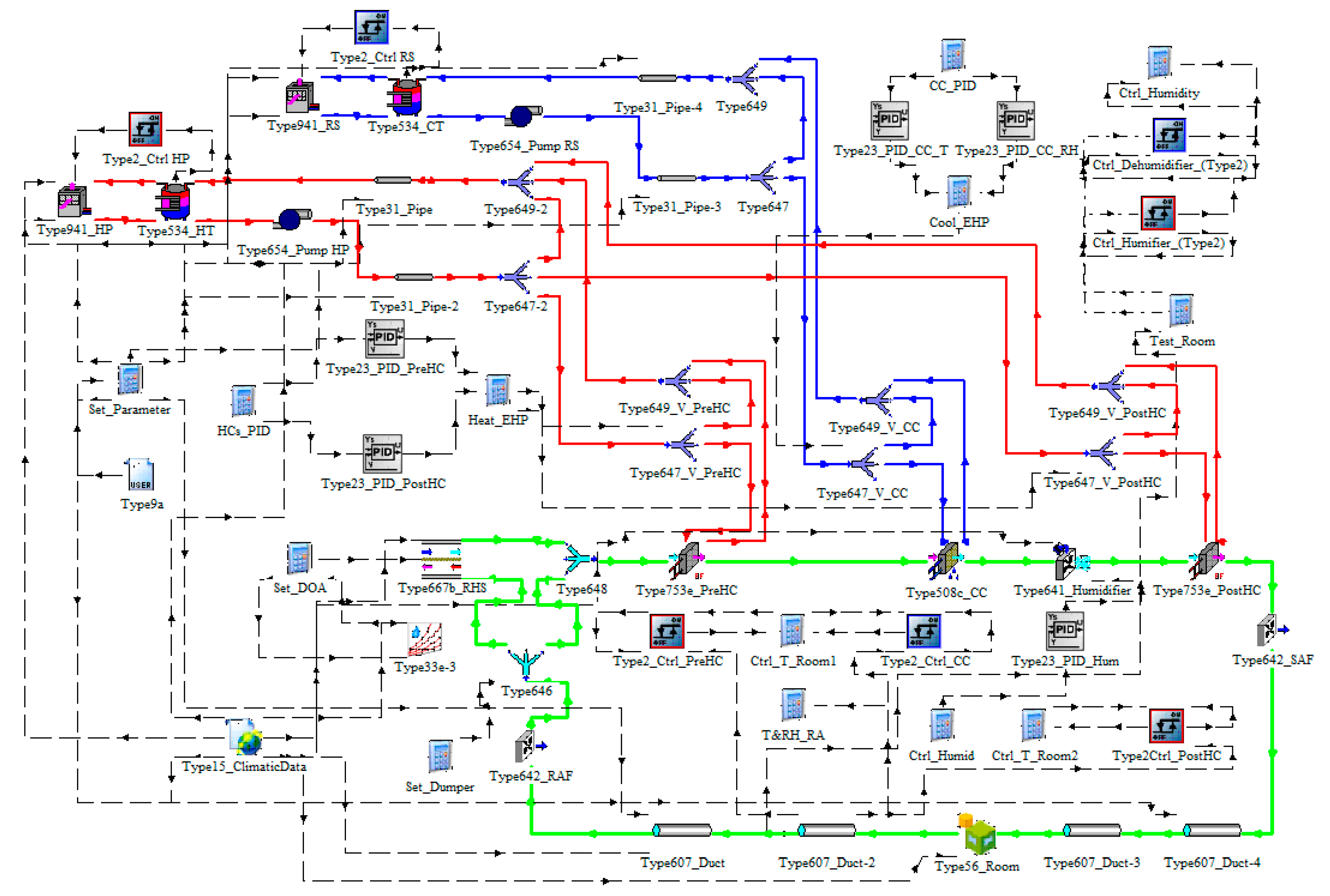
Figure 5 reports a screenshot of the model developed in TRNSYS environment, representing the main circuits by means of different colors. In particular, in this figure the circuit of the hot heat carrier fluid produced by the heat pump and supplying both the pre-heating coil and the post-heating coil has been indicated in red; the circuit of the cold heat carrier fluid produced by the refrigeration unit and supplying the cooling coil has been depicted in blue; finally, the circuit of the moist air through the AHU as well as the test room is highlighted in green. The other TRNSYS Types’ connections are characterized by dashed black lines.

The Type 56 has been considered to take into account the thermal behavior of the integrated test room.

The Type 941 has been adopted to model and simulate the performance of both the refrigeration system (model ANL 050Q [20]) and the heat pump (model ANL 050HQ [20]) serving the AHU of the test room; this model is able to calculate and provide as outputs the cooling power (refrigeration unit), the heating power (heat pump), the power absorbed by the compressor as well as the temperature of both heat carrier fluid and air. The calculation is based on user-supplied data files provided as inputs and containing manufacturer data related to both heating/cooling capacity and power as a function of the outside air temperature and supply fluid temperature. In this study, the performance data measured by the manufacturer [20] and reported in Figure 3a,b have been provided as inputs to the Type 941 in order to calculate the desired outputs.

Both the refrigeration unit as well as the heat pump are equipped with a 75 L thermal energy tank for storing the cold and hot heat carrier fluid, respectively. The Type 534 has been used in this study for modeling the storage. It allows to divide the tanks into fully-mixed sub-volumes; in particular, in this study, 10 isothermal temperature layers have been selected for both storages in order to accurately take into consideration the thermal stratification (the layer 1 is located at the top, while the layer 10 is positioned at the bottom). In particular, the temperature at level 2 of the cold tank has been considered for controlling the operation of the refrigeration unit, while the temperature at level 8 of the hot tank has been used for operating the heat pump.

The Types 753e and 508c have been used for modeling the operation of the post-heating coil and the cooling coil, respectively; in these types, the air is heated/cooled passing over a coil where a hotter/colder heat carrier fluid is flowing. These models use the “bypass fraction approach” to estimate the outlet conditions of both air and fluid; this means that a fraction of the air stream that bypasses the coil is specified (the remaining part of the air stream is completely unaltered by the thermal interaction with the coil); then the bypassed air stream is mixed with the conditioned air stream and these conditions are placed on the coil outlet node. According to the information provided by the manufacturers, a by-pass fraction of 15% has been assumed for the cooling coil, while it has been considered equal to 10% for the post-heating coil.

The humidifier has been simulated with the Type 641, where the outlet air state is defined based on an energy balance by neglecting the heat losses. According to the manufacturer data, a constant power consumption of 3.7 kW has been considered while the humidifier is activated.

Type 667b uses a “constant effectiveness–minimum capacitance” approach to model the air-to-air heat recovery device in which two air streams are passed near each other so that energy may be transferred between the streams. According to the manufacturer’s data, a sensible effectiveness of 79.5%, together with a latent effectiveness equal to 47.0%, have been adopted.

The Type 642 has been considered for modeling the fans, allowing motor heat losses and electric consumption to be taken into the related motor efficiency.

The Type 607 models the geometry of air ducts by considering the heat losses to the surroundings; a thermal resistance of 0.25 m²K/W has been considered for all air ducts in this study. The Type 31 allows the geometry of pipes to be modelled, taking into account the thermal behavior of fluid flow; in this paper, a heat loss coefficient equal to 4.0 W/m²K has been assumed for all pipes.

Types 646 and 648 have been used for modeling the dampers that split an inlet air flow into fractional outlet air flows and vice versa. Types 647 and 649 have been adopted for modeling the valves that split an inlet fluid flow into fractional outlet fluid flows and vice versa.

The control logics for operating the plant components are described in Table 4. They have been implemented by means of on/off differential controllers and Proportional–Integral–Derivative (PID) controllers.

The on/off differential controllers have been modeled by means of Type 2, generating a control function (1 or 0) that is defined depending on both (i) the difference between upper and lower deadband values as well as (ii) the input control function associated to the previous timestep. In this paper, Type 2 has been used to activate/deactivate the heat pump (HP) as well as the refrigerating system (RS) according to the difference between the target and the current level of temperatures inside the hot (level 8) and cold (level 2) tanks, respectively. Type 2 has also been used to activate/deactivate the PID controllers.

Type 23 has been considered for simulating the operation of the PID controllers; these components specify the control signal required to maintain the controlled variables at the target conditions, where the control signals are proportional to the tracking error, as well as to the integral and the derivative of that tracking error. In TRNSYS there are two Types that could be used for modelling the PID controllers: Type 23 and Type 22. In this study, Type 23 has been used instead of Type 22 mainly because of the facts that: (i) Type 22 can operate as an iterative controller only, while Type 23 can operate as a non-iterative or an iterative controller; (ii) the performance of Type 22 is sensitive to some simulation settings (order of components as well as convergence tolerances). The PID controllers operate the valves V_cc (supplying the cooling coil), V_PostHC (supplying the post-heating coil), and V_HUM (supplying the humidifier); the main characteristics of the PID controllers used in this study are described in

Table 8. Main parameters of PID controllers.

Controlled Component of the AHU	Gain Constant	Derivative Time (min)	Integral Time (min)
Humidifier (HUM)	0.03	1	0.1
Cooling coil (CC)	−0.05	1	0.1
Post-heating coil (PostHC)	0.1	1	0.1

.

Type 15, used for modeling the outside climatic conditions, allows to read data at regular time periods from an external weather data file (EnergyPlus) [26] corresponding to the city of Naples (Italy).

Type 33e uses as inputs the dry bulb temperature and relative humidity of moist air and return the other corresponding properties.

5. Model Validation

The model of the HVAC developed in the TRNSYS environment has been validated by contrasting the simulation results with the experimental data described in the previous section. The whole experimental database consists of 1034 points. The simulations have been performed by assuming the following inputs equal to the measured data: desired targets of indoor air temperature (T_SP,Room) and indoor air relative humidity (RH_SP,Room), velocity of return air fan (OL_RAF), supply air fan (OL_SAF), opening percentages of return air damper (OP_DRA), outside air damper (OP_DOA), exhaust air damper (OP_DEA), heat recovery system damper (OP_DHRS), external air temperature (T_OA), deadbands (DB_T and DB_RH) of targets of both indoor air temperature and relative humidity. The simulations have been carried out with a time-step equal to 1 min (according to the measurement frequency). 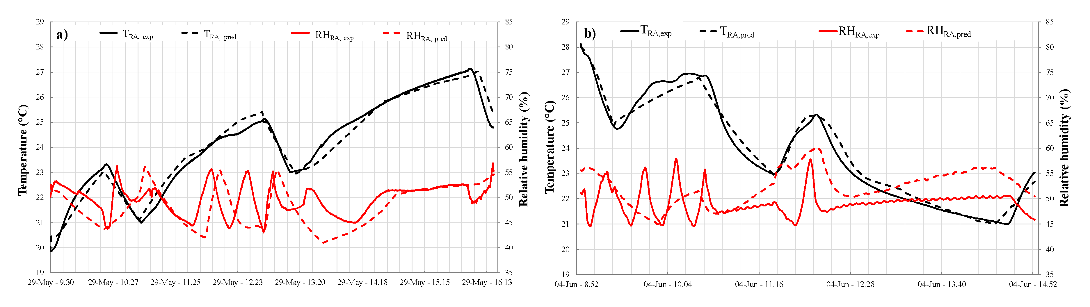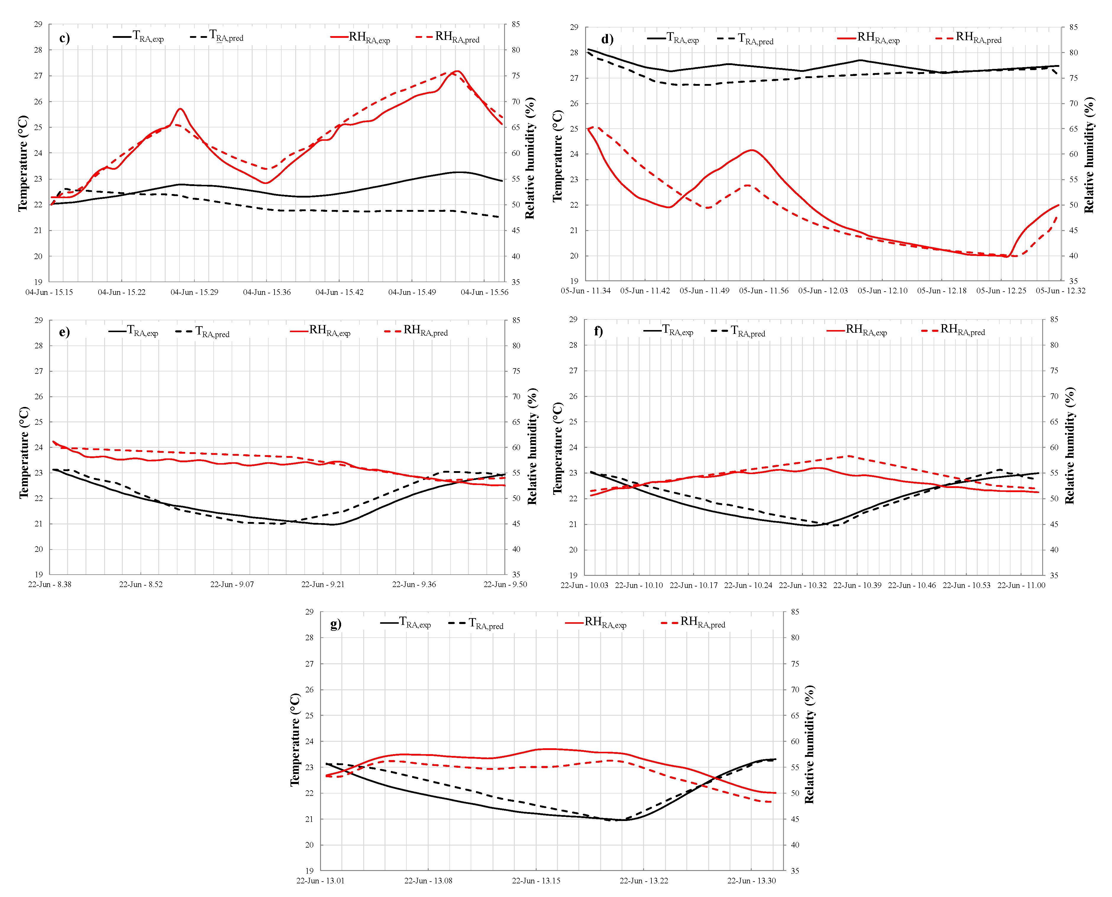Figure 6a–g compare the predicted and experimental outputs in terms of return air temperature (corresponding to the temperature inside the test room) and return air relative humidity (corresponding to the relative humidity inside the test room) for the tests 1, 2, 3, 4, 5, 6, 7 (described in Table 6 and Figure 4), respectively.

The experimental results have been compared with the simulation outputs to assess the accuracy of the calibration by using the following metrics quantifying the instantaneous differences: the average error $\overline{\mathsf{\epsilon }}$; the average absolute error $|\overline{\mathsf{\epsilon }}|$; the root mean square error ε_RMS. These parameters are defined as follows:

$${\mathsf{\epsilon }}_{\mathrm{i}}={\mathrm{g}}_{\mathrm{pred},\mathrm{i}}-{\mathrm{g}}_{\exp ,\mathrm{i}}$$

(1)

$$\overline{\mathsf{\epsilon }}={\displaystyle \sum _{\mathrm{i}=1}^{\mathrm{N}}}{\mathsf{\epsilon }}_{\mathrm{i}}/\mathrm{N}$$

(2)

$$|\overline{\mathsf{\epsilon }}|={\displaystyle \sum _{\mathrm{i}=1}^{\mathrm{N}}}|{\mathsf{\epsilon }}_{\mathrm{i}}|/\mathrm{N}$$

(3)

$${\mathsf{\epsilon }}_{\mathrm{RMS}}=\sqrt{{\sum }_{\mathrm{i}=1}^{\mathrm{N}}\frac{{({\mathsf{\epsilon }}_{\mathrm{i}}-\overline{\mathsf{\epsilon }})}^2}{\mathrm{N}}}$$

(4)

where g_pred,i and g_exp,i are, respectively, the predicted and measured values at time step i and N is the number of points.

Table 9. Errors between the model predictions and measurements.

Test	Number of Experimental Points	Parameter	$\overline{\mathsf{\epsilon }}$	$\mathbf{|}\overline{\mathsf{\epsilon }}\mathbf{|}$	${\mathsf{\epsilon }}_{\mathbf{RMS}}$
Test 1	409	TRA	−0.11 °C	0.32 °C	0.39 °C
		RHRA	−1.64%	3.07%	3.68%
Test 2	359	TRA	−0.07 °C	0.26 °C	0.30 °C
		RHRA	−3.12%	4.06%	3.84%
Test 3	43	TRA	0.62 °C	0.72 °C	0.58 °C
		RHRA	−0.95%	1.39%	1.39%
Test 4	58	TRA	0.32 °C	0.33 °C	0.23 °C
		RHRA	1.05%	3.11%	3.96%
Test 5	74	TRA	−0.16 °C	0.26 °C	0.25 °C
		RHRA	−0.92%	1.27%	1.18%
Test 6	60	TRA	−0.12 °C	0.25 °C	0.27 °C
		RHRA	−1.27%	1.41%	1.31%
Test 7	31	TRA	−0.23 °C	0.36 °C	0.37 °C
		RHRA	1.74%	1.94%	1.79%
Whole database	1034	TRA	−0.05 °C	0.31 °C	0.39 °C
		RHRA	−1.97%	3.26%	3.72%

summarizes the values of $\overline{\mathsf{\epsilon }}$, $|\overline{\mathsf{\epsilon }}|$ and ${\mathsf{\epsilon }}_{\mathrm{RMS}}$.

The maximum instantaneous errors ${\mathsf{\epsilon }}_{\mathrm{i}}$ are about 1.55 °C and about 11.82%, respectively, for T_RA and RH_RA; these deviations are mostly related to a few points occurring during transient operation caused by a change of the desired targets. The results reported in Table 9 highlight that, with reference to the whole database, the values of $\overline{\mathsf{\epsilon }}$, $|\overline{\mathsf{\epsilon }}|$ and ${\mathsf{\epsilon }}_{\mathrm{RMS}}$ are equal to −0.05 °C, 0.31 °C and 0.39 °C, respectively, for T_RA and equal to −1.97%, 3.26% and 3.72%, respectively, for RH_RA. The lowest values of ${\mathsf{\epsilon }}_{\mathrm{RMS}}$ in terms of T_RA and RH_RA correspond, respectively, to test 4 and test 5; the largest values of ${\mathsf{\epsilon }}_{\mathrm{RMS}}$ in terms of T_RA and RH_RA are associated, respectively, to tests 3 and 4. The deviations between measured and simulated data are fully coherent with the accuracy of the instruments, demonstrating that predicted outputs agree very well with experimental observations. Therefore, it can be stated that the model gives an accurate representation of the dynamic and steady-state HVAC performance and it can also be usefully adopted in combination with FFD methods for the detection of any non-optimal states of HVAC systems under predictive maintenance programs.

6. Faults Analysis and Results

In this section, the experimental performance (described in the Section 3) has been simulated by intentionally introducing 6 different typical soft faults into the operation of the HVAC; the simulations have been performed by running the calibrated and validated model described in the previous Section 5, while assuming the values of the following inputs equal to the experimental data measured during the tests performed on the AHU operating under normal condition: external air temperature T_OA, air temperature T_BEA and relative humidity RH_BEA around the room, target room temperature T_SP,Room and target room relative humidity RH_SP,Room, temperature deadband DB_T, relative humidity deadband DB_RH, velocity of the return air fan OL_RAF, velocity of the supply air fan OL_SAF, opening percentage of the exhaust air damper OP_DEA, opening percentage of the outside air damper OP_DOA, opening percentage of the return air damper OP_DRA and opening percentage of the heat-recovery system damper OP_DHRS. Then, the experimentally measured performances of the AHU operating without faults have been compared with those associated to the operation in the cases of faults occurrence. The comparison has been performed in order to (i) analyze the specific behaviors of key parameters associated to each fault, and (ii) assess the differences in terms of thermo-hygrometric comfort hours as well as electric energy consumption caused by the fault occurrence.

Even though each component of an AHU can be potentially corrupted by a fault, the most common faults can affect sensors (e.g., offset in the measurement), controlled devices (e.g., blockage or leakage of air damper or coil valves), equipment (e.g., coil fouling or reduced capacity, duct leakage, fan complete failure or deviation in the pressure drop or belt slippage) and controllers (e.g., unstable or frozen control signal for dampers, coils or fan) [27]. In particular, in this paper the following 6 typical soft faults, which are independent of each other, have been taken into account:

Fault 1):

positive offset of return air temperature sensor (+2 °C);

Fault 2):

negative offset of return air temperature sensor (−2 °C);

Fault 3):

positive offset of return air relative humidity sensor (+10%);

Fault 4):

negative offset of return air relative humidity sensor (−10%);

Fault 5):

return air damper is stuck (fully closed);

Fault 6):

outside air damper is stuck (fully closed).

Fault 1 means that the measured return air temperature is 2.0 °C higher than the true value; fault 2 means that the measured return air temperature is 2.0 °C lower than the right value; fault 3 means that the measured return air relative humidity is 10.0% higher than the true value; fault 4 means that the measured return air relative humidity is 10.0% lower than the true value; fault 5 means that the return air damper is stuck in the fully closed position; fault 6 means that the outside air damper is stuck in the fully closed position.

Figure 7, Figure 8, Figure 9, Figure 10, Figure 11 and Figure 12 report the differences between normal operation and faulty operation in terms of return air temperature T_RA, supply air temperature T_SA, return air relative humidity RH_RA and supply air relative humidity RH_SA as a function of the time. In particular, the following parameters are reported in Figure 7, Figure 8, Figure 9 and Figure 10:

$$\Delta {\mathrm{T}}_{\mathrm{RA}}={\mathrm{T}}_{\mathrm{RA},\mathrm{pred},\mathrm{w}/\mathrm{o}\_\mathrm{fault}}-{\mathrm{T}}_{\mathrm{RA},\mathrm{pred},\mathrm{fault}}$$

(5)

$$\Delta {\mathrm{T}}_{\mathrm{SA}}={\mathrm{T}}_{\mathrm{SA},\mathrm{pred},\mathrm{w}/\mathrm{o}\_\mathrm{fault}}-{\mathrm{T}}_{\mathrm{SA},\mathrm{pred},\mathrm{fault}}$$

(6)

$$\Delta {\mathrm{RH}}_{\mathrm{RA}}={\mathrm{RH}}_{\mathrm{RA},\mathrm{pred},\mathrm{w}/\mathrm{o}\_\mathrm{fault}}-{\mathrm{RH}}_{\mathrm{RA},\mathrm{pred},\mathrm{fault}}$$

(7)

$$\Delta {\mathrm{RH}}_{\mathrm{SA}}={\mathrm{RH}}_{\mathrm{SA},\mathrm{pred},\mathrm{w}/\mathrm{o}\_\mathrm{fault}}-{\mathrm{RH}}_{\mathrm{SA},\mathrm{pred},\mathrm{fault}}$$

(8)

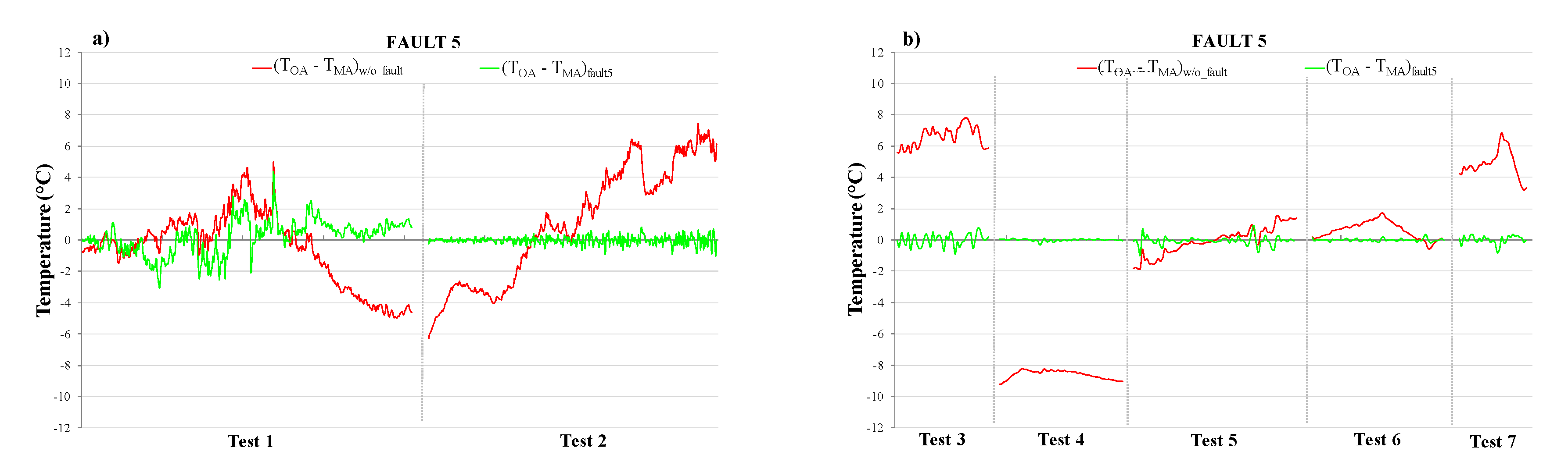
where T_{RA,pred,w/o_fault}, T_{SA,pred,w/o_fault}, RH_{RA,pred,w/o_fault}, RH_{SA,pred,w/o_fault}, are, respectively, the predicted values under normal operation, while T_{RA,pred,fault}, T_{SA,pred,fault}, RH_{RA,pred,fault}, RH_{SA,pred,fault} represent the predictive values in the case of fault occurrence. In Figure 11 the difference (T_OA,pred-T_MA,pred) between the predicted outside air temperature T_OA,pred and the predicted temperature of the air entering the supply air filter T_MA,pred, with and without the occurrence of faults 5, are reported. 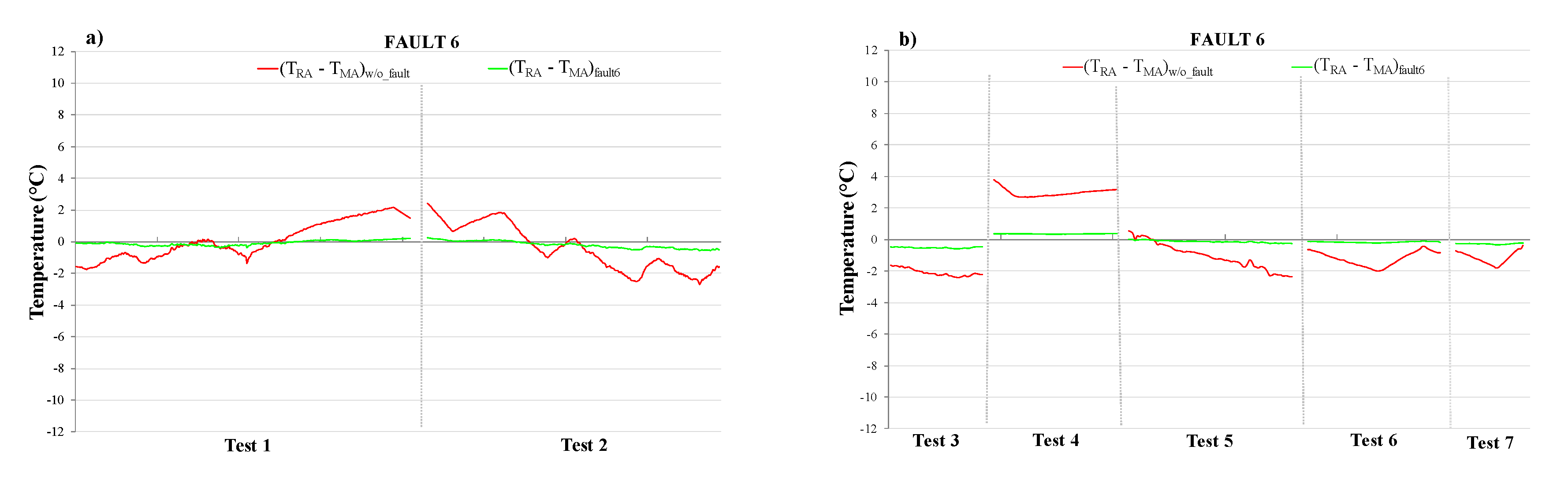Figure 12 shows the difference (T_RA,pred-T_MA,pred) between the predicted return air temperature T_RA,pred and the predicted temperature of the air entering the supply air filter T_MA,pred, with and without the occurrence of faults 6. Figure 7a, Figure 8a, Figure 9a, Figure 10a, Figure 11a and Figure 12a refer to the operating conditions of the experimental tests 1 and 2 (see Table 6), while Figure 7b, Figure 8b, Figure 9b, Figure 10b, Figure 11b and Figure 12b correspond to the boundary conditions of the experimental tests 3, 4, 5, 6 and 7 (see Table 6). Each figure reports the experimental trends obtained in the case of operation without faults in comparison with the trends of the same key parameters while only one of the aforementioned 6 faults is occurring. The target values of both the indoor air temperature T_SP,room and relative humidity RH_SP,room are also reported in the same figures.

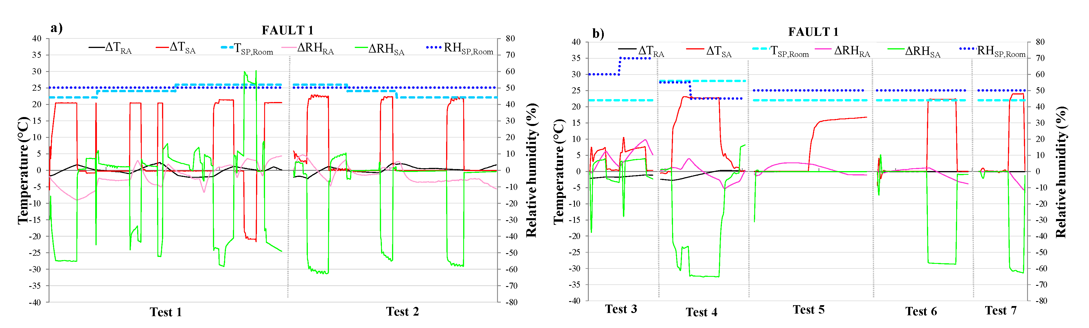
The trends of key parameters under fault 1 are reported in Figure 7a (tests 1 and 2) and Figure 7b (tests 3, 4, 5, 6 and 7). It can be noticed that, in the case of fault 1, the difference ΔT_SA is positive during about 61.5% of the whole simulation time (with T_{SA,pred,w/o_fault} up to about 24 °C larger than T_{SA,pred,fault1}), while the difference ΔRH_SA is negative during about 58.1% of the whole tests period (with RH_{SA,pred,w/o_fault} about 62% lower than RH_{SA,pred,fault1}). In the case of fault 1 occurrence, it can be also underlined that the controllers require a 19.1% and 10.8% longer operating time of cooling coil and humidifier, respectively, causing an increase (+8.5%) in terms of electric energy consumption associated to the operation of the refrigerating system as well as the preparation of steam flow. However, this case is also characterized by a 7.1% shorter operating time of post-heating coil (thanks to the fact that the measured T_RA is larger than the real one), reducing the electric energy consumed by the heat pump (−14.6%).

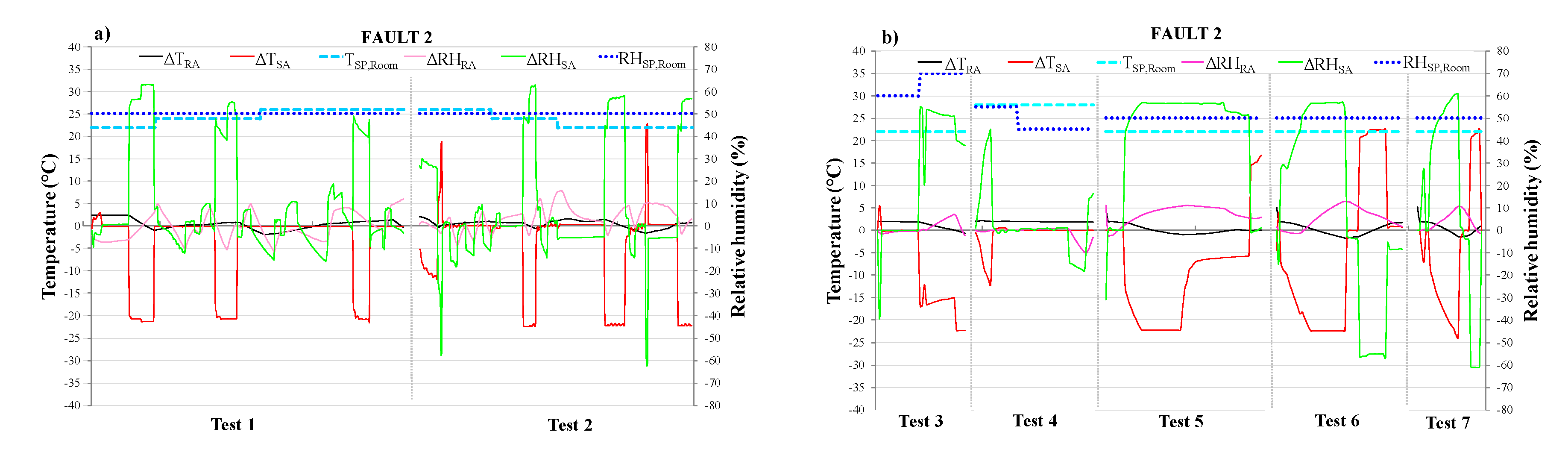
The trends associated to key parameters under fault 2 are indicated in Figure 8a (tests 1 and 2) and Figure 8b (tests 3, 4, 5, 6 and 7). The results highlight that, in the case of the fault 2, the difference ΔT_SA is negative during about 75.5% of the whole simulation time (with T_{SA,pred,w/o_fault} up to about 24 °C lower than T_{SA,pred,fault2}), while the difference ΔRH_SA is positive during about 55.0% of the whole tests duration (with RH_{SA,pred,w/o_fault} about 64% greater than RH_{SA,pred,fault2}). In the case of fault 2 occurrence, it can be also noticed that the controllers require a 14.3% longer operating time of post-heating coil, causing a greater electric energy consumption associated to the heat pump (+26.8%); however, in this case, the operating time of cooling coil and humidifier are reduced by about 18.9% and 32.6% (thanks to the fact that the measured T_RA is lower than the real one), lowering the related electricity consumption (−19.7%).

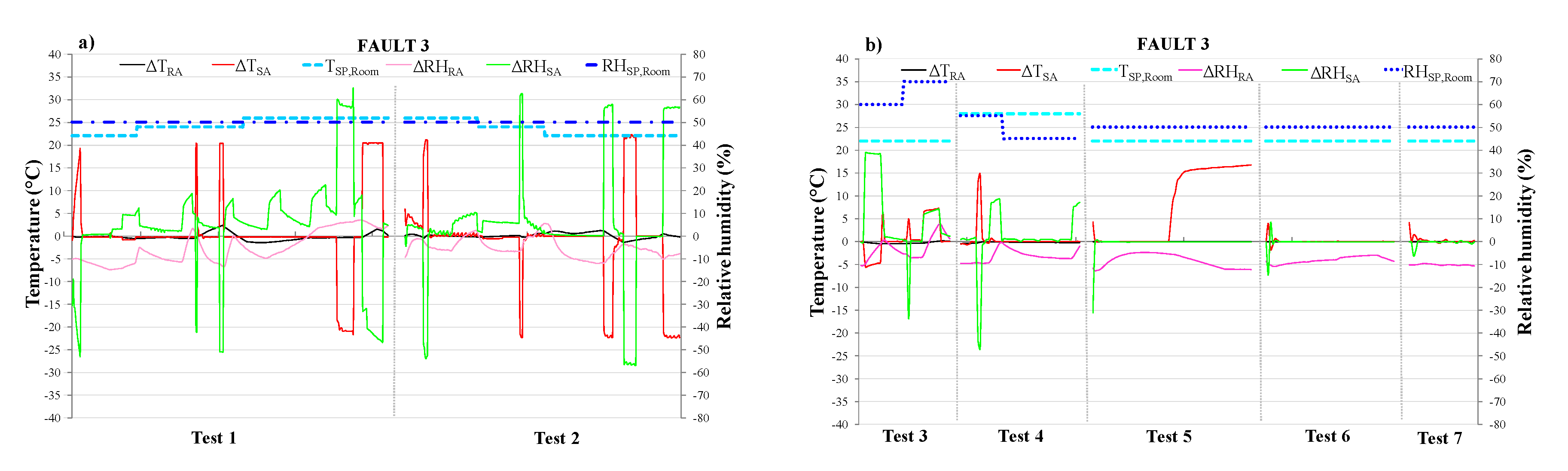
The trends of key parameters under fault 3 are highlighted in Figure 9a (tests 1 and 2) and Figure 9b (tests 3, 4, 5, 6 and 7). The simulations indicate that, in the case of fault 3, the difference ΔRH_RA is negative during about 83.0% of the whole simulation time (with RH_{RA,pred,w/o_fault} up to about 21% lower than RH_{RA,pred,fault3}), while the difference ΔRH_SA is positive during about 83.1% of the tests duration (with RH_{SA,pred,w/o_fault} up to about 64% greater than RH_{SA,pred,fault3}); in this case, the controllers require a 11.4% shorter operating time of humidifier, reducing the related electric energy consumption (−25%) (thanks to the fact that the measured RH_RA is higher than the real one); however, in this case the operating time of the cooling coil is 17.3% longer, causing a larger electricity demand of the refrigerating system (+5.2%).

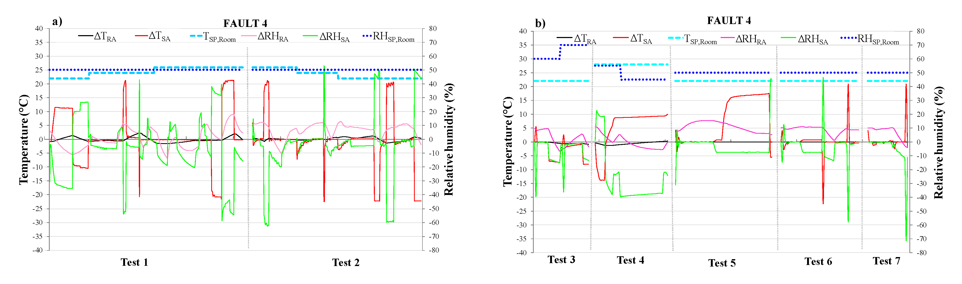
The trends associated to key parameters under the fault 4 are indicated in Figure 10a (tests 1 and 2) and Figure 10b (tests 3, 4, 5, 6 and 7). The simulation data underline that, in the case of the fault 4, the difference ΔRH_RA is positive during about 70.4% of the whole simulation time (with RH_{RA,pred,w/o_fault} up to about 18.1% greater than RH_{RA,pred,fault4}), while the difference ΔRH_SA is negative during about 81.0% of the tests duration (with RH_{SA,pred,w/o_fault} up to about 62.6% greater than RH_{SA,pred,fault4}); in this case, the controllers require a small variation of operating time of post-heating coil (about +6.8% of the whole simulation time), whereas there is a significant increase of about 35.2% in the operating time of the humidifier (causing a significant increment of the associated electric energy consumption (+48.3%)), together with a decrease of about 21.3% in the operating time of the cooling coil (causing a slight decrement of the associated electric energy consumption (−2.1%) thanks to the fact that the measured RH_RA is higher than the real one).

The trends associated to key parameters under fault 5 are reported in Figure 11a (tests 1 and 2) and Figure 11b (tests 3, 4, 5, 6 and 7). The results provided by the simulation model highlight that, in the case of the fault 5, the difference (T_OA,pred-T_MA,pred)_fault5 is close to zero; in particular, this difference is in the range −0.5–0.5 °C for about 69% of the whole simulation time (while the difference (T_OA,pred-T_MA,pred)_{w/o_fault} is in the same range for about 17.3% only of the tests duration_, reaching a maximum absolute value of about 9.2 °C). This fault causes a slightly longer operating time of cooling coil and humidifier, respectively, together with a slightly shorter operating time of the post-heating coil.

The trends associated to key parameters under fault 6 are indicated in Figure 12a (tests 1 and 2) and Figure 12b (tests 3, 4, 5, 6 and 7). The simulation data underline that, in the case of fault 6, the difference (T_RA,pred-T_MA,pred)_fault6 is always close to zero; in particular, this difference is in the range −0.5–0.5 °C for about 96% of the whole simulation time (while the difference (T_RA,pred-T_MA,pred)_{w/o_fault} is in the same range for about 19.1% only of the tests duration_, with the maximum absolute value equal to about 3.8 °C). This fault causes shorter electric energy consumption with respect to the normal operation; in particular, the controllers require a slightly shorter operating time of post-heating coil and humidifier, respectively, together with a slightly longer operating time of cooling coil.

The data reported in Figure 7, Figure 8, Figure 9, Figure 10, Figure 11 and Figure 12 show that performance differences between the operations with and without faults are often significantly consistent (mainly in the cases of faults 1 and 2); therefore, even if additional analyses and investigations have to be performed over a wider range of boundary conditions, it can be stated that specific rules could be potentially identified in order to detect/predict the presence of non-optimal states of the HVAC operation.

7. Case Study

A typical small-size office building located in the city of Naples (southern Italy, latitude: 40°51′22″ N, longitude: 14°14′47″ E) is assumed as case-study to be served by the air-handling unit described in the Section 2. The building, with a total area of 18 m² and a volume of 54 m³, is characterized by a flat roof with only one floor; there are two West and East oriented windows with a total area of 1.8 m² together with a thermal transmittance of 1.40 W/m²K. The characteristics of the building envelope are shown in

Table 10. Building envelope characteristics of the office.

Component of Office Building Envelope	Layer Material (from Outside to Inside)	Thickness (m)	Thermal Conductivity (W/mK)	Conductive Thermal Resistance (m2K/W)		Area (m2)
Horizontal ceiling	Bitumen	0.008	0.170	0.047	3.095	18.0
	Screed	0.050	0.085	0.588
	Reinforced concrete slab	0.050	0.850	0.059
	Hollow brick	0.200	0.247	0.810
	Expanded polystyrene	0.050	0.032	1.563
	Lime plaster	0.020	0.700	0.029
Horizontal floor	Concrete slab	0.200	0.150	1.333	2.732	18.0
	Concrete subfloor	0.100	0.730	0.137
	Expanded polystyrene	0.040	0.032	1.250
	Tiles	0.012	1.000	0.012
Vertical walls	Cement plaster	0.020	0.900	0.022	2.896	13.5–12.0
	Hollow brick	0.250	0.195	1.282
	Expanded polystyrene	0.050	0.032	1.563
	Lime plaster	0.020	0.700	0.029

, selected according to the threshold values imposed by Italian legislation requirements. The office is empty during the weekends, while in weekdays there is a constant number of 3 people working from 8:00 am to 6:00 pm. The working activity is characterized by an internal sensible and latent gain of 65 W/occupant and 55 W/occupant, respectively; the heat gains due to 3 PCs (420 W), a laser printer (110 W) and artificial lighting systems (3.75 W/m²) are taken into account. The target of indoor air temperature (T_SP,Room) is set to 20 °C (±1 °C) during the heating period (1 November–31 March) and 26 °C (±1 °C) during the cooling period (1 April–31 October); the target of relative humidity (RH_SP,Room) is always set to 50% (±5%) during the entire year. The AHU system can operate to achieve the targets only when at least one occupant being inside the office.

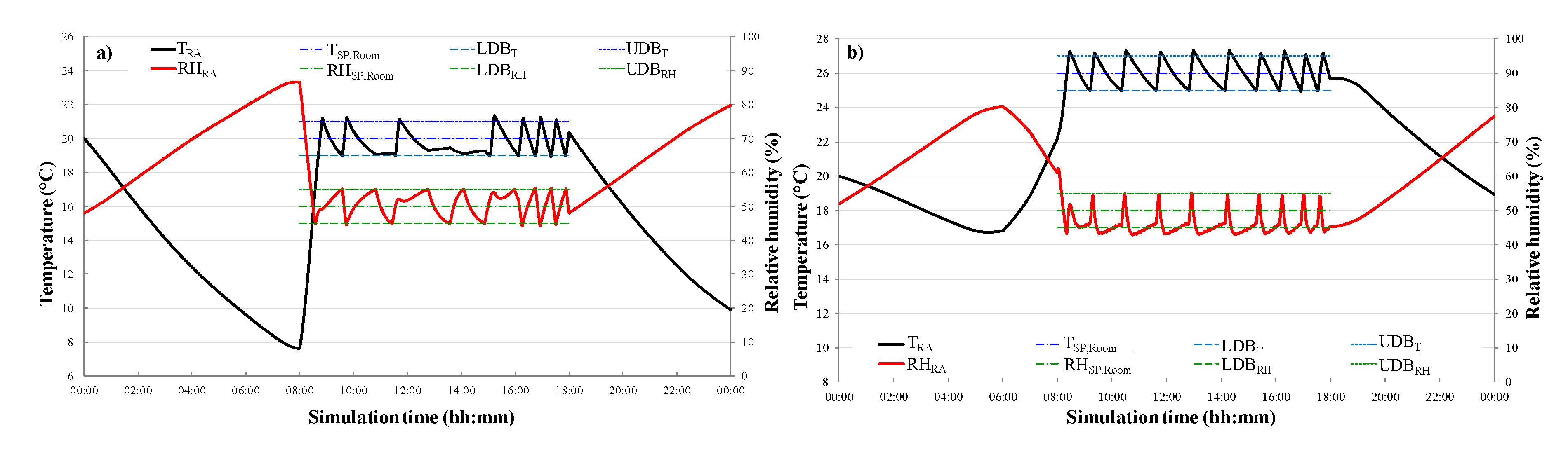
The performance of the system under normal operation (without faults) is firstly analyzed. In particular, Figure 13a,b show the daily profiles of return air temperature (T_RA) and return relative humidity (RH_RA), together with the lower (LDB) and upper (UDB) deadbands of return air temperature and relative humidity, for two selected days (1 February and 1 July) of the simulation period during heating and cooling seasons.

Table 11. Percentage of thermo-hygrometric comfort time and electric energy consumption during heating, cooling and whole year without faults.

Simulation Period	Thermal Comfort Time (%)	Hygrometric Comfort Time (%)	Electric Energy Consumption (kWh)
Heating period	84.7	80.4	6291.1
Cooling period	84.4	83.9	11496.0
Whole year	84.5	82.5	17787.1

highlights the thermal comfort time (i.e., the percentage of time during which the target of indoor air temperature is achieved), the hygrometric comfort time (i.e., the percentage of time during which the desired target of indoor air relative humidity is achieved), and the overall electric energy consumption due to the operation of the refrigerating system, the heap pump, the humidifier as well as the supply and return air fans.

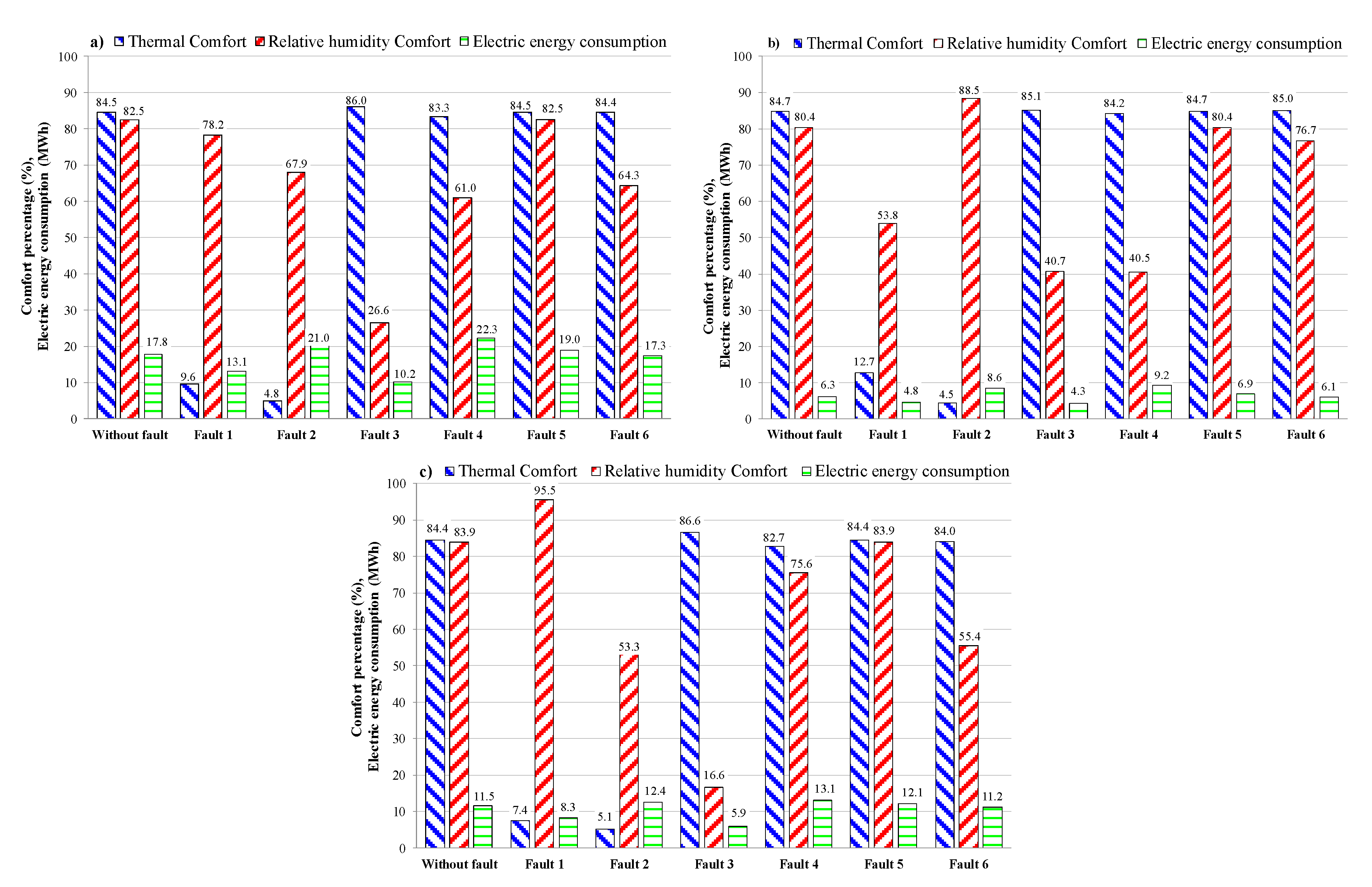
Figure 14 highlights the thermal comfort hours, the hygrometric comfort hours as well as the overall electric energy consumption, for both the case without faults and the cases when one the six aforementioned faults occurs in order to facilitate the comparison among the different scenarios. In particular, Figure 14a–c refer to the whole year, the heating period only and the cooling period only, respectively. These figures highlight that the thermal comfort hours and hygrometric comfort hours represent 84.5% and 82.5%, respectively, of the entire operation time of the AHU with reference to the scenario without faults. In comparison to the performance under normal operation:

• the thermal comfort time in the case of occurrence of the fault 1 is decreased by a large amount (from 84.5% down to 9.6% with reference to the entire year), together with a slight reduction of the annual hygrometric comfort time; whatever the period is, fault 1 is characterized by a lower (−26.5%) electricity demand thanks to the reduced operating time of post-heating coil and heat pump (due to the fact that the measured T_RA is larger than the real one);
• whatever the period, the occurrence of fault 2 significantly deteriorates the comfort of occupants taking into account that it greatly reduces the thermal comfort time (from 84.5% down to 4.8% with reference to the entire year) as well as the hygrometric comfort time (from 82.5% down to 67.9% with reference to the entire year); fault 2 causes a larger (+18.1%) electric energy consumption due to a longer operating time of post-heating coil (associated to the fact that the measured T_RA is lower than the real one);
• whatever the period, the occurrence of the faults 3 and 4 substantially decreases the hygrometric comfort time from 82.5% down to 26.6% and 61.0%, respectively, during the entire year (while the thermal comfort time remains almost constant); fault 3 is characterized by a lower (−42.5%) electric energy consumption thanks to a shorter operating time of humidifier (due to the fact that the measured RH_RA is larger than the real one); fault 4 causes a larger (+25.4%) electric demand due to a longer operating time of the humidifier (associated to the fact that the measured RH_RA is lower than the real one);
• whatever the period is, the thermal and hygrometric comfort hours remain almost constant in the case of fault 5 occurrence, while the overall electric energy consumption increases (+6.7%);
• whatever the period, the effect of fault 6 is almost negligible on thermal comfort time; the hygrometric comfort hours decrease, together with a slight reduction (−2.8%) in terms of overall electric energy consumption.
• The values reported in these figures highlight that, with respect to the normal operation, the occurrence of the aforementioned 6 faults could significantly affect the thermo-hygrometric comfort and/or the overall electric energy consumption; therefore, developing systems and procedures for predictive maintenance programs able to promptly detect and/or predict any non-optimal states of HVAC operation could substantially help in maintaining the desired indoor thermo-hygrometric conditions as well as lowering the inefficient usage of electricity associated with faulty operation.

8. Conclusions

The application of automated fault detection and diagnostics (FDD) under HVAC predictive maintenance programs requires the development of simulation models able to accurately compare the faulty operation with respect to nominal conditions. In this paper, a detailed dynamic simulation model of an existing HVAC system has been developed; the predictions of the model have been contrasted with the measured data, highlighting the capability of the model to represent the dynamic and steady-state HVAC performance (root mean square errors lower than 0.39 °C and 3.72%, respectively, in predicting the measured indoor air temperature and relative humidity) and, therefore, to be usefully applied in combination with FFD methods.

Six different typical soft faults have been intentionally introduced into the validated model and the operation of the HVAC system has been simulated; the analysis of dynamic trends of key parameters associated to faulty conditions in comparison to normal performance allowed confirmation that simplified rules could be identified to promptly detect and/or predict any non-optimal states of HVAC devices. In particular, the simulation results highlighted that:

-

in the case of positive offset of return air temperature sensor (+2 °C), the values of T_SA associated to the normal operation are larger than the values corresponding to the faulty operation during about 61.5% of the time;

-

in the case of negative offset of return air temperature sensor (−2 °C), the values of T_SA associated to the normal operation are lower than the values corresponding to the faulty conditions during about 75.5% of the time;

-

in the case of positive offset of return air relative humidity sensor (+10%), the values of RH_RA associated to the normal operation are greater than the values corresponding to the faulty operation during about 83.0% of the time;

-

in the case of negative offset of return air relative humidity sensor (−10%), the values of RH_RA associated to the normal operation are lower than the values corresponding to the faulty conditions during about 70.4% of the time;

-

in the case of the return air damper being stuck (fully closed), the difference (T_OA,pred-T_MA,pred) is in the range −0.5–0.5 °C for about 69% of the time;

-

in the case of the outside air damper being stuck (fully closed), the difference (T_RA,pred-T_MA,pred) is in the range −0.5–0.5 °C for about 96% of the time.

Finally, the impacts associated to the occurrence of the aforementioned faults have been assessed with reference to the case study of a typical Italian building office; the results underlined that faulty operation could significantly affect the thermo-hygrometric comfort of occupants as well as the overall electric energy consumption. In particular, the negative offset of the return air temperature sensor (−2 °C), the negative offset of the return air relative humidity sensor (−10%) and the stuck of the return air damper significantly enhance the electric energy consumption (from a minimum of 6.7% up to a maximum of 25.4%), while the positive offset of return air temperature sensor (+2 °C), the positive offset of return air relative humidity sensor (+10%) and the stuck of the outside air damper result in a reduction of electricity demand (from a minimum of −2.8% up to a maximum of −42.5%). The annual thermal comfort time is decreased by a large amount (from 84.5% down to 9.6%) in the case of positive offset of return air temperature sensor (+2 °C); the negative offset of return air temperature sensor (−2 °C) significantly reduces the annual thermal comfort time (from 84.5% down to 4.8%). The occurrence of positive and negative offset of return air relative humidity sensor greatly decreases the hygrometric comfort time from 82.5% down to 26.6% and 61.0%, respectively, during the entire year.

Therefore, developing HVAC predictive maintenance programs could substantially help in maintaining the desired indoor thermo-hygrometric conditions as well as lowering the inefficient usage of electricity associated to faulty operation.