Article

The Value of PV Power Forecast and the Paradox of the “Single Pricing” Scheme: The Italian Case Study

1
Department of Enterprise Engineering, University of Rome Tor Vergata, 00133 Rome, Italy
2
EURAC Research, Institute for Renewable Energy, Viale Druso, 1, 39100 Bolzano, Italy
3
Atmospheric Sciences Research Center, State University of New York, Albany, NY 12203, USA
4
CHOSE, University of Rome Tor Vergata, 00133 Rome, Italy
*
Author to whom correspondence should be addressed.
Energies 2020, 13(15), 3945; https://doi.org/10.3390/en13153945
Submission received: 1 July 2020 / Revised: 23 July 2020 / Accepted: 29 July 2020 / Published: 1 August 2020

Abstract

:
One of the major problem of photovoltaic grid integration is limiting the solar-induced imbalances since these can undermine the security and stability of the electrical system. Improving the forecast accuracy of photovoltaic generation is becoming essential to allow a massive solar penetration. In particular, improving the forecast accuracy of large solar farms’ generation is important both for the producers/traders to minimize the imbalance costs and for the transmission system operators to ensure stability. In this article, we provide a benchmark for the day-ahead forecast accuracy of utility scale photovoltaic (PV) plants in 1325 locations spanning the country of Italy. We then use these benchmarked forecasts and real energy prices to compute the economic value of the forecast accuracy and accuracy improvement in the context of the Italian energy market’s regulatory framework. Through this study, we further point out several important criticisms of the Italian “single pricing” system that brings paradoxical and counterproductive effects regarding the need to reduce the imbalance volumes. Finally, we propose a new market-pricing rule and innovative actions to overcome the undesired effects of the current dispatching regulations.

1. Introduction

In Italy, over 20 years, the electric mix has evolved from 20% to 35% worth of renewable energy (RE) generation and, in only 10 years, solar became the second most prevalent RE source after hydropower (Figure 1a). According to the 2030 climate and energy framework, adopted by the European Council in October 2014, the Italian National Energy Strategy (SEN) [1] and the Integrated National Plan for Energy and Climate (PNEC or PNIEC (both the acronyms can be found in literature)) [2] prescribe 55% of the electricity demand to come from RE sources and define how this target can be reached in Italy (Figure 1a). The growth of RE penetration (i.e., the fraction of annual demand covered by renewable sources) should be driven by wind and solar generation (Figure 1b). Wind generation has to increase from the current 17.2 TWh/year to 40 TWh/year, while solar production from 24.4 TWh/year to 74.5 TWh/year. In this way, by 2030, the photovoltaic (PV) penetration (which is already one of the highest in Europe [3] and the third in the world [4]) will increase from 8% to 22%, becoming the first Italian RE source.
Nevertheless, a large share of photovoltaic generation imposes new challenges for the national energy system. One of the major problems related to the PV grid integration is the increase in the imbalances between supply and demand due to the intrinsic solar intermittency and stochastic variability. Indeed, since PV generation is not programmable and, if distributed mainly locally in terms of production and consumption, the supply of programmable energy sources needed to fulfill the residual electric demand becomes much more difficult to predict. As a result, the growth of the PV penetration will increase dramatically with the solar-induced imbalances and a higher amount of flexible and dispatchable capacity (reserves) would have to be held to ensure the security and stability of the national grid.
Figure 2 shows an example of the impact of the forecast errors on the imbalance and the energy volumes that must be exchanged on the balancing energy market (BEM) to resolve this imbalance. In this case, a clear sky day was erroneously predicted so that the Italian transmission system operator (TSO) had to purchase a remarkable amount of energy on the BEM for upward regulation to compensate this underprediction.
For this reason, the PNEC explicitly states that, with the achievement of the 2030 RE objectives, “the high quantity of non-programmable renewable sources will force to keep available a significant portion of thermoelectric generation capacity, in order to guarantee the necessary reserve margins for the safe operation of the system”.
The Italian transmission system operator (Terna Spa) is the largest TSO in Europe. It is responsible for the security and the stability of the whole 72,900 km of the national transmission grid. Currently, only large photovoltaic producers that manage plants with a capacity greater than or equal to 10 MW have to deliver their day-ahead power forecast to Terna and, according to the “single pricing” rule, are subject to penalties for the imbalance between their real and scheduled generation. In contrast, Terna manages the remaining distributed PV (customer-sited) plants in an aggregate manner and the imbalance costs are borne to ratepayers. Even if, nowadays, the majority of solar generation comes from the distributed PV fleet, the improvement of the forecast accuracy for large solar farms is important for two main reasons:
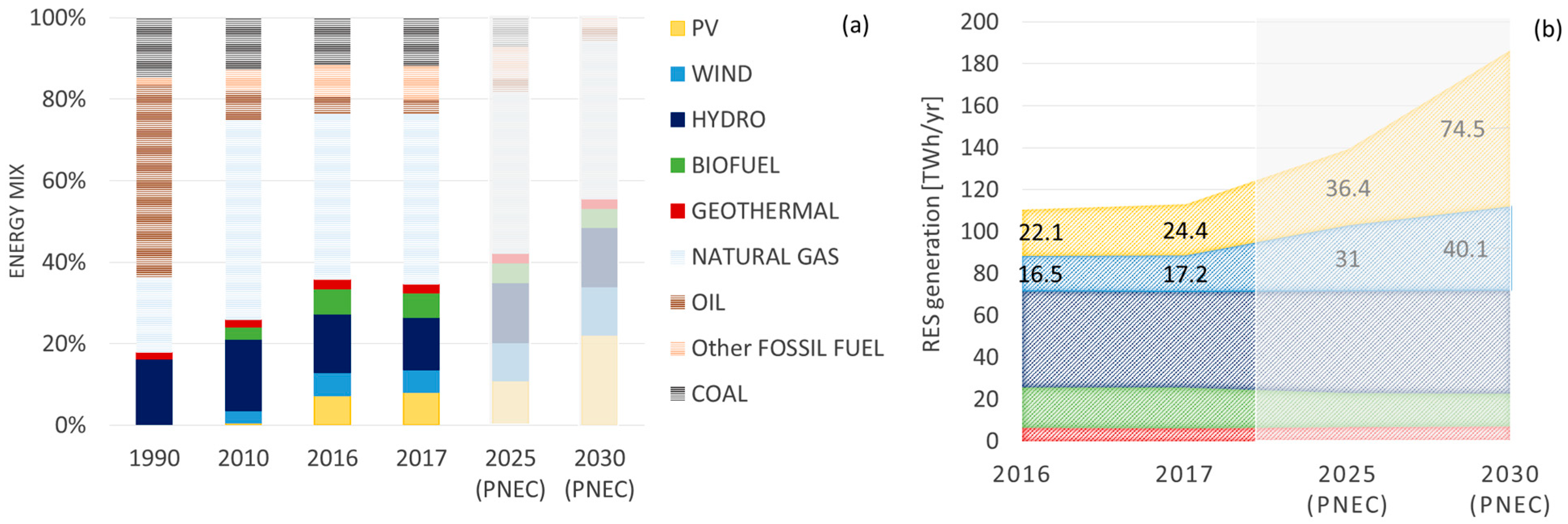
  • The objective of the PNIEC by 2030 will inevitably require an increase in the capacity of utility scale PV plants with respect to the distributed one and in fact, we now have tenders to cover this part although at the moment only wind projects are presented to problems in getting building permits for PV plants.
  • To predict the day-ahead supply and reserves, Terna needs to forecast the whole Italian PV generation. The forecast model is strongly based on the large plant generation scheduling: “Terna receives the forecast from several external suppliers, subject to a pre-qualification process and continuous performance monitoring, who make their own forecasts … Before the execution of each sub-stage of the planning phase, the individual forecasts are then processed, together with the final photovoltaic production … by a statistical algorithm of “meta-forecasting”, which provides the best combination of the different forecasts, in order to minimize the overall forecast error” [7].
Therefore, in order to achieve the 2030 solar generation target, it is necessary not only to implement policies to promote a rapid increase in photovoltaic installations (centralized and distributed) but also to ensure an appropriate balancing regulatory framework that economically rewards the most accurate forecasting of large photovoltaic parks’ generation.
The first aim of this work is to benchmark the forecast accuracy of the generations of large PV farms, their related imbalance values and the value of the accuracy improvement in 1325 locations all over Italy. The second aim is to assess the effectiveness of the current energy market framework to boost large solar producers/traders to increase the performance of their forecast and hence to reduce their solar-induced imbalances. Therefore, this study is important, not only for the owners of solar farms to understand the value of accurate solar predictions, but also for the Italian TSO and policy makers (Italian Authority for Energy/Minister of Economic Development) to understand the limits of the current energy market regulation framework.
The paper is organized as following:
  • In Section 2, we report the novelty of work with respect to the existing literature
  • In Section 3, we summarize the main features of the Italian energy market and of the solar imbalance regulation framework
  • In Section 4, we present the satellite and numerical weather prediction data employed to estimate and forecast the generation of utility scale PV plants all over Italy
  • In Section 5, we describe the methodology used to carry out our study
  • In Section 6, we report the main accuracy and economic metrics used to assess the forecast performance and its related imbalance economic value for large solar producers/traders
  • In Section 7, we discuss the results emerging from our investigation. We show the forecast accuracy of the photovoltaic generation of utility scale solar plants on 1325 locations in Italy and we compute the imbalance values of their forecasts. These values are compared with those obtained with a baseline forecast to evaluate the economic advantage of the forecast accuracy improvements
  • In Section 8, we suggest a possible market regulation revision
  • In Section 9, conclusions are reported

2. Existing Literature and Novelty of the Work

In the last years several works have centered on assessing the value of PV power forecasting and forecast accuracy improvement both from the point of view of transmission and distribution system operators (regional fleet forecasts) and from the producers’/traders’ point of view (single plant forecasts).
Zhang et al. [8] studied the economic benefits of improving the forecast accuracy of the regional solar generation for the Independent System Operator-New England (ISO-NE) and for the California-ISO (CAISO). They found that, according to the local balancing energy markets (BEMs), with more accurate forecasts, the two different ISOs can achieve a 25% reduction in reserve costs. Brancucci et al. [9] computed the economic impacts of solar generation on the grid management costs for the ISO-NE. From the analysis of operational electricity generation, electricity generation from the fast start and lower efficiency power plants, ramping of all generators, start and shutdown costs, and solar power curtailment cost, the authors derive the values of forecast accuracy improvement at different penetration levels. Wu et al. [10] quantify the additional reserve costs induced by solar/wind variability and uncertainty, in the case of the Arizona Public Service Company utility in the southwestern United States. Joos et al. [11] suggest possible reforms of the German and UK balancing regulation systems to reduce wind and solar integration costs. Pierro et al. in [12,13] evaluate the energy and economic benefit for a local distribution system operator in the north of Italy in improving their TSO transmission scheduling and reducing the reserves by the use of accurate probabilistic PV generation forecasts. In [14], Pierro et al. extend these studies to the Italian national scale, proposing an innovative strategy to reduce the imbalance and its related costs. The authors, first, assess the value of improving the PV power prediction accuracy by the use of “state of the art” forecast models and the enlargement of the forecast-controlled area. Afterward, they propose the use of a new kind of solar system, called “flexible” PV plants, able to provide dispatching services for solar-induced imbalance regulations by proactive curtailment and battery storage additional power. These studies [12,13,14] were conducted considering the current and future solar penetration at regional and national levels. Perez et al. [15,16] showed how flexible plants can be used at first to provide a “perfect forecast”, removing the prediction uncertainty and then providing a full dispatchable, firm PV generation 24/365, removing solar intermittency for several US states. The costs of turning all the PV fleets into flexible systems depend essentially on the size of the battery energy storage systems and if they are economically affordable in the near future. Fonseca et al. [17] studied the reduction in PV curtailment that can be achieved in Japan by the use of a perfect PV power forecast obtained by solar plants equipped with battery energy storage systems (BESS) instead of a traditional day-ahead PV power forecast derived by numerical weather prediction (NWP) products. Nevertheless, the authors used a purely theoretical perfect forecast (using actual production data in lieu of forecasts) without computing the BESS capacity (needed to reach a perfect prediction) and its related costs.
At single site level, Kaur et al. in [18] quantified the forecast value for the owner of a one MW PV farm in the Western Interconnection dispatch energy mark. De Giorgi et al. [19] and Bignucolo et al. [20] quantified the imbalance costs or revenues that can be achieved by the owners of a 960 kWp PV and 3.6 MW wind farms under the Italian “single pricing” scheme. Nevertheless, in [19], De Giorgi et al. assumed the energy markets prices to be constant during the year; therefore, the resulting economic evaluation is rather limited. In [20], Bignucolo et al. focused their attention more on the benefit of using battery energy storage systems to reduce the wind imbalance and maximize the revenues on the dispatching market. It is worth noting that, in [15], Perez et al. also evaluate the value of a “perfect forecast” achievable by the proactive curtailment and battery energy storage at the PV site level in climatically distinct individual US locations. Furthermore, the authors analyzed the differences between the standard accuracy metric and a new operational metric that quantifies the lowest cost of operationally, achieving “perfect forecasts”.
Antonanzas et al. [21] analyzed the imbalance economic valorization and the values of forecast improvement of a 1.86 MWp PV plant derived from the “dual pricing” rule on the Iberian balancing energy market. The authors used different PV power forecast methods, and as in [15], they pointed out the discrepancies between the standard accuracy metrics and economic metrics for choosing the best prediction method.
Finally, a comparison between the “single pricing” and the “dual pricing” mechanisms in the Italian market zone of Sicily, can be found in [22]. Even if many simplified assumptions are assumed and a simple forecast model is used, the relative comparison between the imbalance costs achievable by the two market rules can be considered an interesting result.
First, unlike the works [8,17], the present study is aiming to quantify the forecast accuracy and its economic value for PV producers/traders that manage utility scale PV farms. However, the reported results are important both for the Italian TSO and for the Italian Authority for Energy/Minister of Economic Development in charge of the energy market regulation framework. Moreover, differently from [15,20], we consider the imbalance only of traditional solar farms that do not make use of any battery energy storage.
The first novelty of this work is to provide an accurate benchmark of the day-ahead PV power imbalance (forecast accuracy) and of its related cost on the energy market all over Italy with a resolution of 12 × 12 km. As far as the authors know, this kind of study is novel and does not exist for any country in Europe.
While in [22] the impact of “single” and “dual” pricing mechanisms on the PV imbalance costs are analyzed, in this paper we consider only the current “single” pricing market rule. In contrast, our results are much more reliable since we use an accurate forecast method and real hourly market prices of the period 2014–2016.
Among the cited works, the one of Antonanzas et al. [21] presents more similarities to our investigation. In [21], the authors assess the values of different forecast methods while we test just one PV prediction model. In contrast, they performed their study at a single location and for a small period (half a year), while we conducted the analysis on 1325 different locations for three different years (2014–2016). Therefore, our results not only are more statistically meaningful, but also point out more critical features of the current market’s regulatory framework: the second major contribution of the study.

3. Spot Market Structure and Imbalance Regulatory Framework for Production Units in Italy

3.1. Spot Market Structure

To ensure the security of the Italian electricity system, the 20 Italian regions have been aggregated into six areas defined by the physical energy transit limits of the national transition grid [23]: North (NORD); Center-North (CNOR); Center-South (CSUD); South (SUD); Sicily (SICI) and Sardinia (SARD (Figure 3). These areas each feature a spot energy market in which most of the energy needed to fulfill the national demand is exchanged.
The spot market is organized into three main energy submarkets: the day-ahead market (DAM), intra-day market (IDM) and balancing energy market (BEM). The BEM is divided into two: the market of the dispatching services (MSD ex-ante) and the real time balancing market (BM). Each submarket is characterized by different functions, gate open/closure time, the number of sections, and different energy price formation rules.
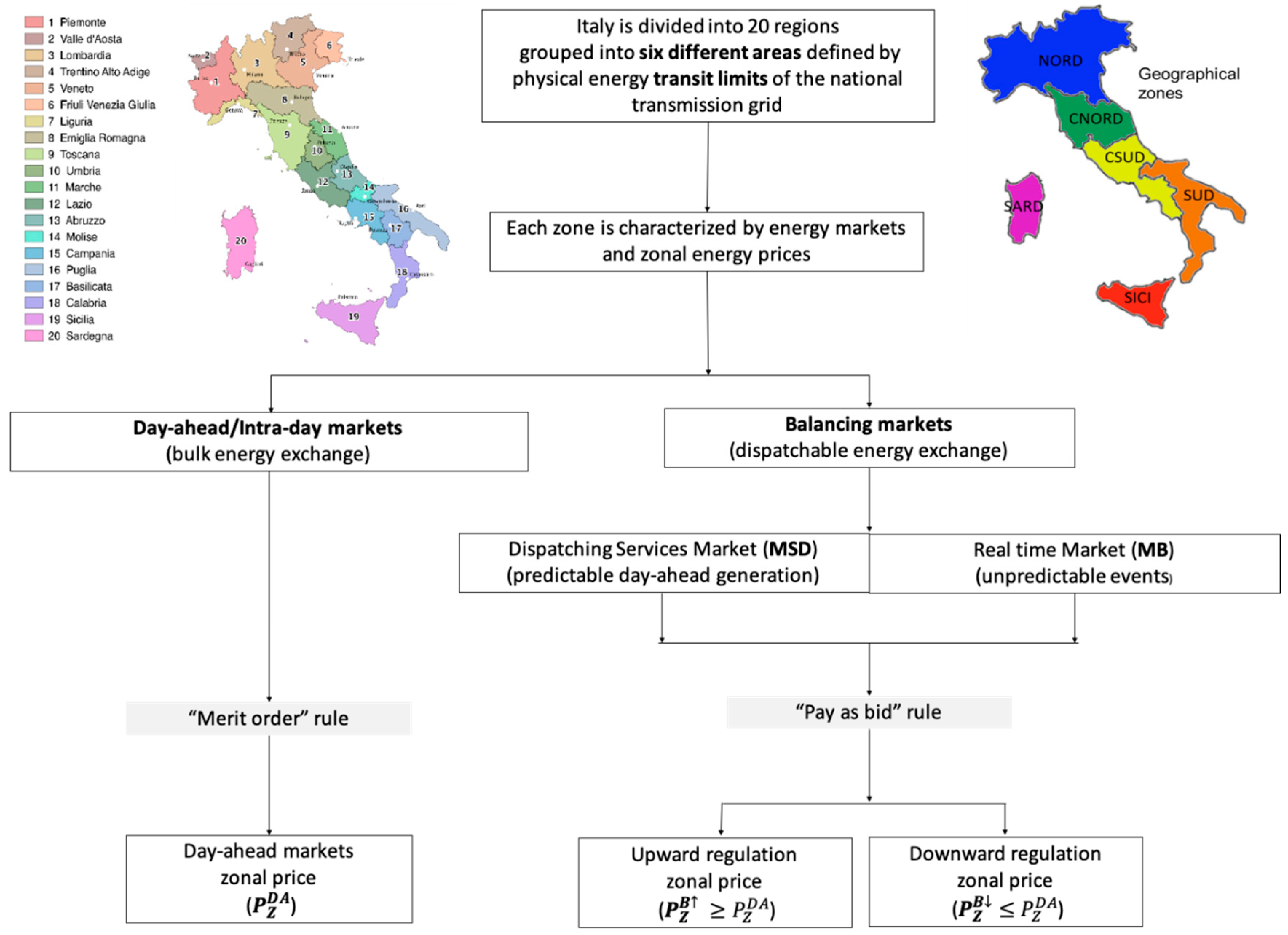
  • The DAM is the place of negotiation for the bulk supply/purchase electricity bids for each hour of the delivery day. All electrical operators can participate in the DAM. The bids are accepted by the Italian Energy Services Manager (GME) according to the “Merit Order” rule that will define the energy price, i.e., the equilibrium price between supply/purchase bids. If accepted, the energy of the supply bid is remunerated at the zonal price (P_Z^DAM) while the energy of the purchased bid at the single national price (PUN). The PUN is the average zonal price weighted over the relative amount of exchanged energy. Accepted bids determine the preliminary scheduling for the energy supply and withdrawal of each grid connection point for the day of delivery. The zonal prices depend on the transit capacity limits between the market zones according to the Italian TSO (Terna) requirement [24].
  • The IDM is the place of negotiation for the supply/purchase electricity exchange for each hour of the current day, with the purpose of adjusting the injection/withdrawal scheduling defined by the DAM.
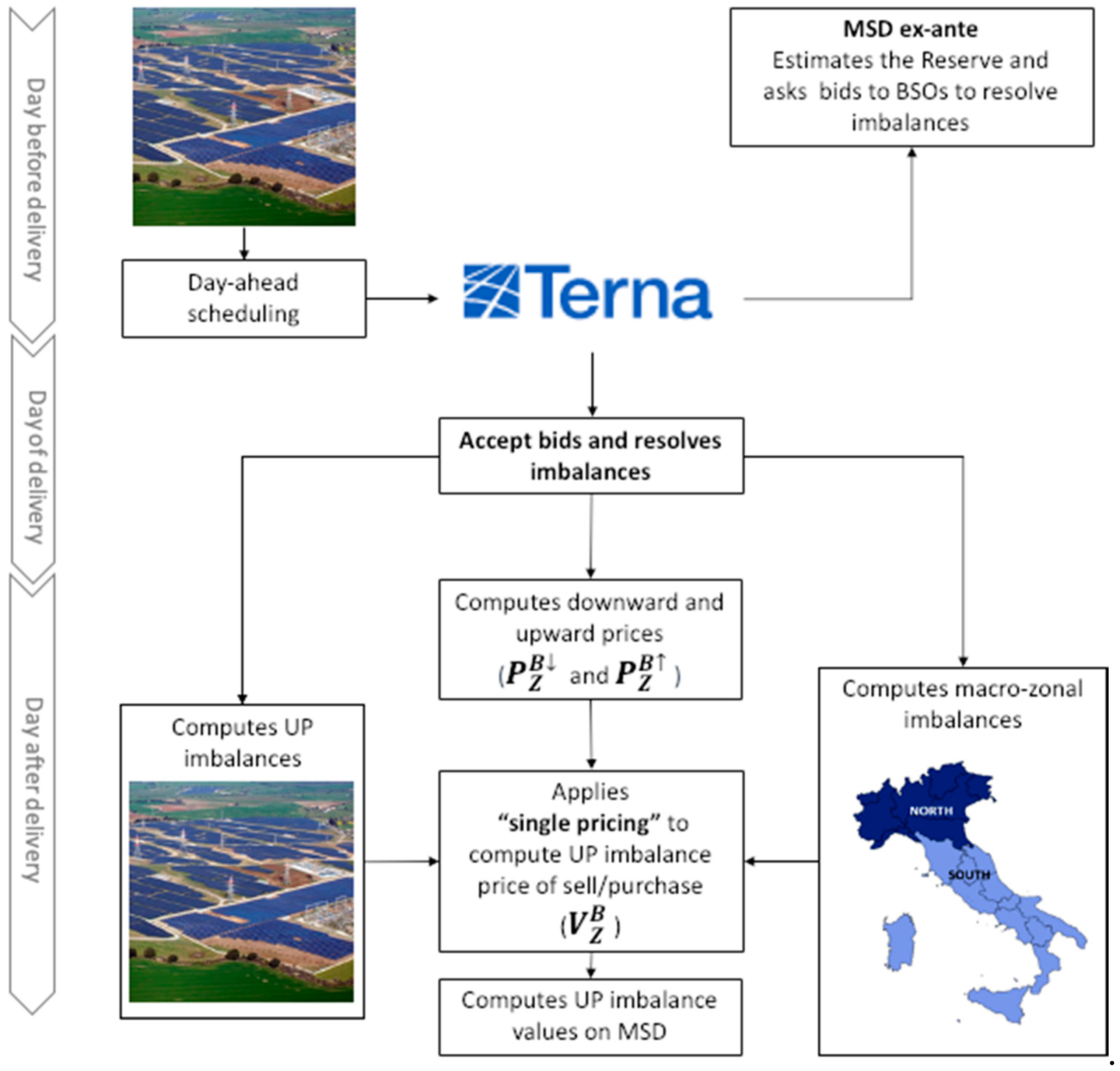
  • The BEM is the place for the negotiation of bids for the supply/purchase of dispatching services, used by Terna for the resolution of intra-zonal congestions, for the supply of the reserves and for the balancing in real time between demand/supply. The BEM is divided into two: the market of the dispatching service (MSD ex-ante) and the real time balancing market (MB). On the MSD ex-ante, Terna defines the reserves margin and acquires/sells the energy needed to compensate the day-ahead imbalance and to resolve congestions. On MB, Terna acquires/sells in real time (by sending dispatching orders) and the energy is needed to correct the imbalance due to unpredictable events or errors in the reserve estimation
On the BEM, Terna acquires/sell dispatchable energy following the “Pay as Bid” role, i.e., bids are accepted based on simple economic merit. On the balancing energy market, two different prices appear: an upward regulation price ( P Z B ) in case of there being less of the supply than predicted (negative zonal imbalance) and a downward regulation price ( P Z B ) in case of having more of the supply than predicted (positive zonal imbalance). The first price is equal to or higher than the DAM price with no upper limit, while the second is equal to or lower than the DAM price with zero as the lower limit. These energy prices are the average zonal prices of the accepted bids weighted with the corresponding exchanged energy and they are defined ex-post the day after the day of balancing energy delivering [24].

3.2. Production Unit Imbalance and Economic Valorization on MSD

According to the regulatory framework 281/2012/R/efr, 525/2014/R/EEL, 419/2017/R/eel of the Italian Authority for Electricity and Gas and the dispatch guidelines of Terna [25], the production units (UP) are divided into: relevant or non-relevant. The relevant UP are single plants or aggregated plants of the same type in a given zone (virtual production units) with a total capacity greater than 10 MW.
Only “relevant” UPs have to deliver to the TSO the day-ahead generation scheduling and will incur in penalties for the imbalances with respect to their scheduled profile. The generation imbalance is defined as:
E i m b M S D ( U P , h ) = E g e n e r a t i o n c u r r e n t ( U P , h ) E g e n e r a t i o n f o r e c a s t ( U P , h )
where E g e n e r a t i o n c u r r e n t and E g e n e r a t i o n f o r e c a s t are the real and day-ahead scheduled generation of the UP at the delivery hour ( h ).
Therefore, a UP negative imbalance means underproduction with respect to the scheduling, while positive imbalance means overproduction.
To define the energy price of the relevant UP imbalance, Terna divided Italy into two macro-zones (Table 1). The first is the North market zone and the second is the remaining part of Italy.
The price of the generation imbalance of the relevant UPs depends on the sign of the regional imbalance of the macro-zone in which the UP is located: a negative zonal imbalance means less supply than needed while a positive zonal imbalance occurs when the supply exceeds the demand. The macro-zones sign is computed by Terna ex-post (after the supply) so that the price of the “relevant” UPs imbalance is also known ex-post.
A subset of the relevant production units is enabled to participate on the dispatching market depending on the flexibility and programmability of their power generation (balancing system operators (BSO)) [25]. In particular, variable renewable power plants, such as wind and solar plants, are not allowed to provide dispatching services. The imbalance price for these variable energy plants is defined by the “single pricing” rule, i.e., the price on the BEM depends only on the sign of macro-zonal imbalance (Table 1). This rule has been designed to take into account the effect of the imbalance of the single “relevant” UP on the overall imbalance of the macro-zone (in which the UP is located).
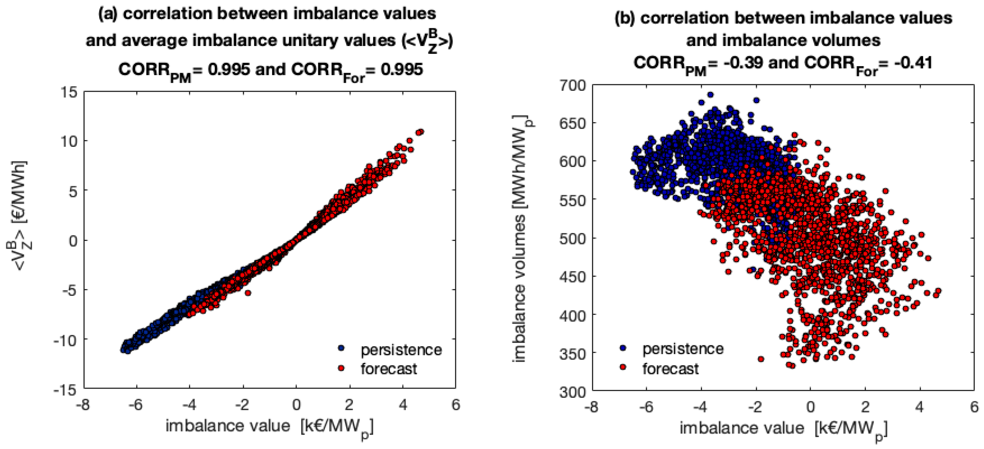
  • If the signs of the imbalance are the same, the day-ahead generation scheduling errors of the “relevant” solar farm contribute to an increase in the imbalance of the macro-zone. In this case, the imbalance value will be negative, i.e., a cost for the producer.
  • If the imbalance signs are different, the scheduling errors contribute to reduce the macro-zone imbalance and the imbalance value will be positive, i.e., a revenue for the producer.
Figure 4 shows the main statistical values (mean, one and two std and out-layers) of the DAM and MSD prices during 2014–2016 together with the imbalance price resulting from the “single pricing” rule. It is worth noting that the mean imbalance price is similar to the mean day-ahead price but the range of variability is much wider, reaching values up to 1000 EUR/MWh for the critical upward regulation hour.
Figure 5 summarizes the whole process to compute the UP imbalance values.
It is important to specify that the imbalance cost borne by “relevant” UPs allowed to provide ancillary services (BSO) is defined by the “dual pricing” market scheme in which the imbalance price depends on both the zonal and UP imbalance signs (dual), this scheme is well explained in [21,26]. In contrast with the “single pricing”, this rule cannot produce revenues for balancing system operators.

4. Satellite and Numerical Weather Prediction Data

The satellite and numerical weather prediction data have been provided by the forecast provider Ideam Srl. A brief description of these data is reported below.

4.1. Satellite Derived Data

The satellite derived irradiance (GHI) used for power estimation comes from the geostationary radiative fluxes products, under Météo-France’s responsibility. It was obtained by the OSI SAF SSI algorithm applied to the satellite images provided by METEOSAT-9 (MSG-3) at 0° longitude, covering 60 S–60 N and 60 W–60 E, at 0.05° latitude–longitude. The data have an hourly granularity and a spatial resolution of 12 km × 12 km—amounting to 1325 grid points for the entire country.
A particularity of the Météo-France data is to report the GHI equal at zero at a sun elevation lower than 10°. Thus, to reduce this error the data were post-processed with a cubic extrapolation of the clear sky index for low sun elevation angles. Each of the 1325 time series covers the period 2014–2017 (Figure 6b).

4.2. Numerical Weather Prediction Forecast Data

The GHI and Tair prediction, used as the forecast model’s input, were generated by the Weather Research and Forecasting model (WRF-ARW 3.8) [27] with an initialization at 12 UTC, analyzing the 24 h forecasts starting from the following 00 UTC:
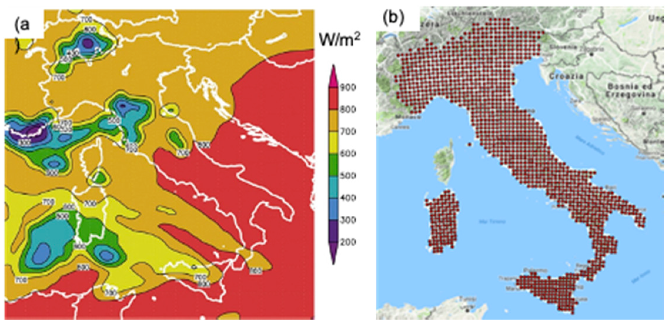
  • The initial contour data for model initialization comes from the GFS model output with a spatial resolution of 12 km × 12 km (Figure 6)
  • Radiation scheme: “Rapid Radiative Transfer Model”
  • Forecast horizon: 24 h/temporal output resolution: 1 h/spatial resolution 12 km × 12 km covering all the country (1325 points)
  • Each of the 1325 daily hindcasts time series covered the period 2014–2017
Importantly, we observed that the WRF irradiance predictions exhibited considerable bias errors. Indeed, in most of the radiation schemes used by the WRF model, the GHI is sensibly reduced only if one or more vertical model levels present the water vapor content at the saturation level. In cases where the forecasted relative humidity of the entire column is very close to, but not at, the saturation point, the modeled GHI reduction is very weak. This ignores the fact that, in real atmospheres, there is almost certainly condensation of the water vapor at some height, with a consequent GHI reduction at the surface [28]. Moreover, other factors limit the capabilities of the radiation scheme. For instance, in our case, aerosols and gas concentrations are set by tables that only take into account the time of year and location. Consequently, the variation of diffuse and direct components due to these aspects is rigid and predefined. For these reasons, we had to correct the irradiance prediction obtained by the WRF with an original model output statistic method based on deterministic and neural network model chains similar to the one we had previously developed and described in [29]. However, the description of this method is out of the scope of this work.

5. Materials and Methods

In order to benchmark the economic value of the solar energy trading on the MSD ex-ante and day ahead (DA) energy markets, and to verify the effectiveness of the current market regulation in encouraging PV producers to reduce their imbalances, we adopted the following methodology (Figure 7):
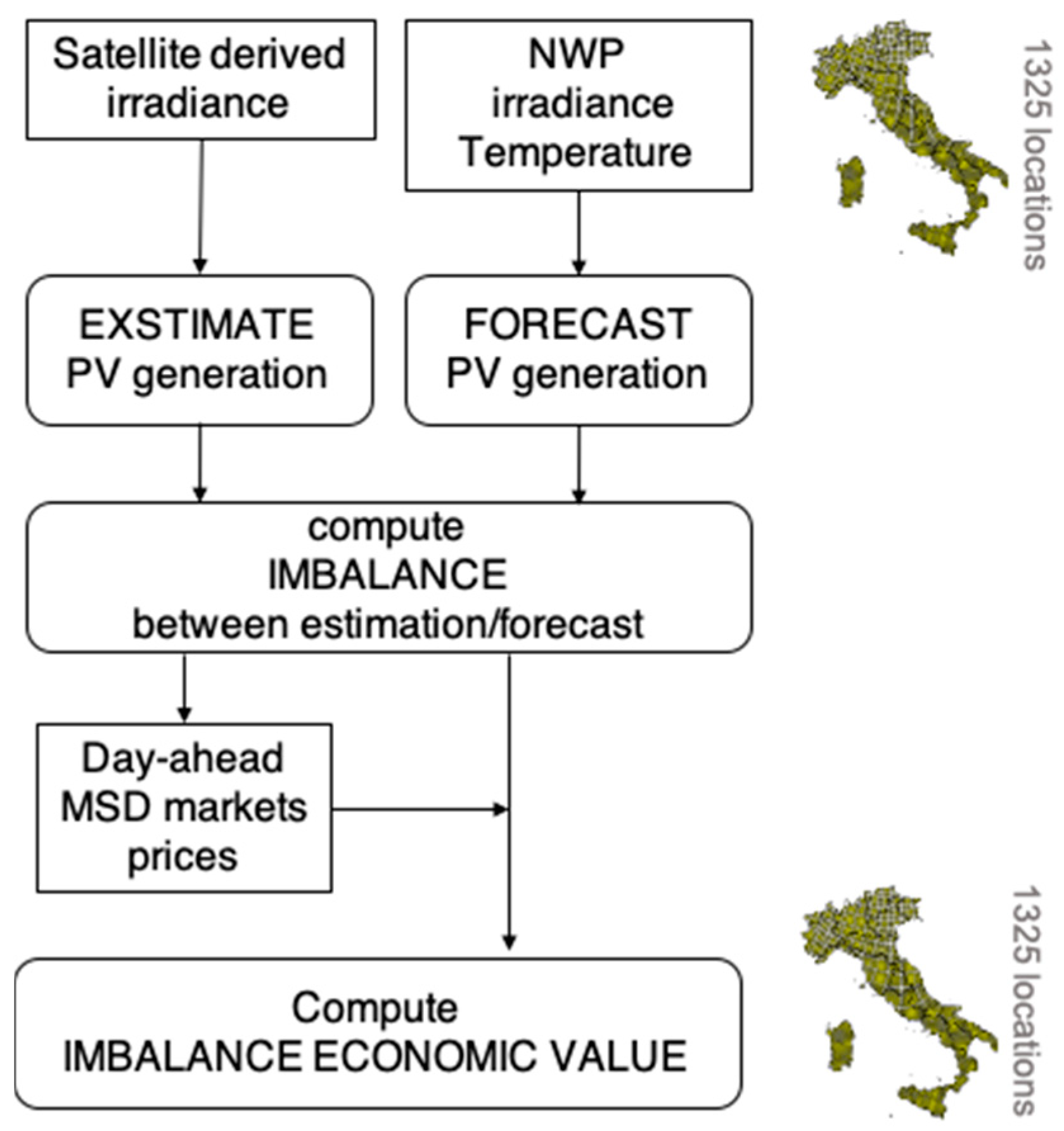
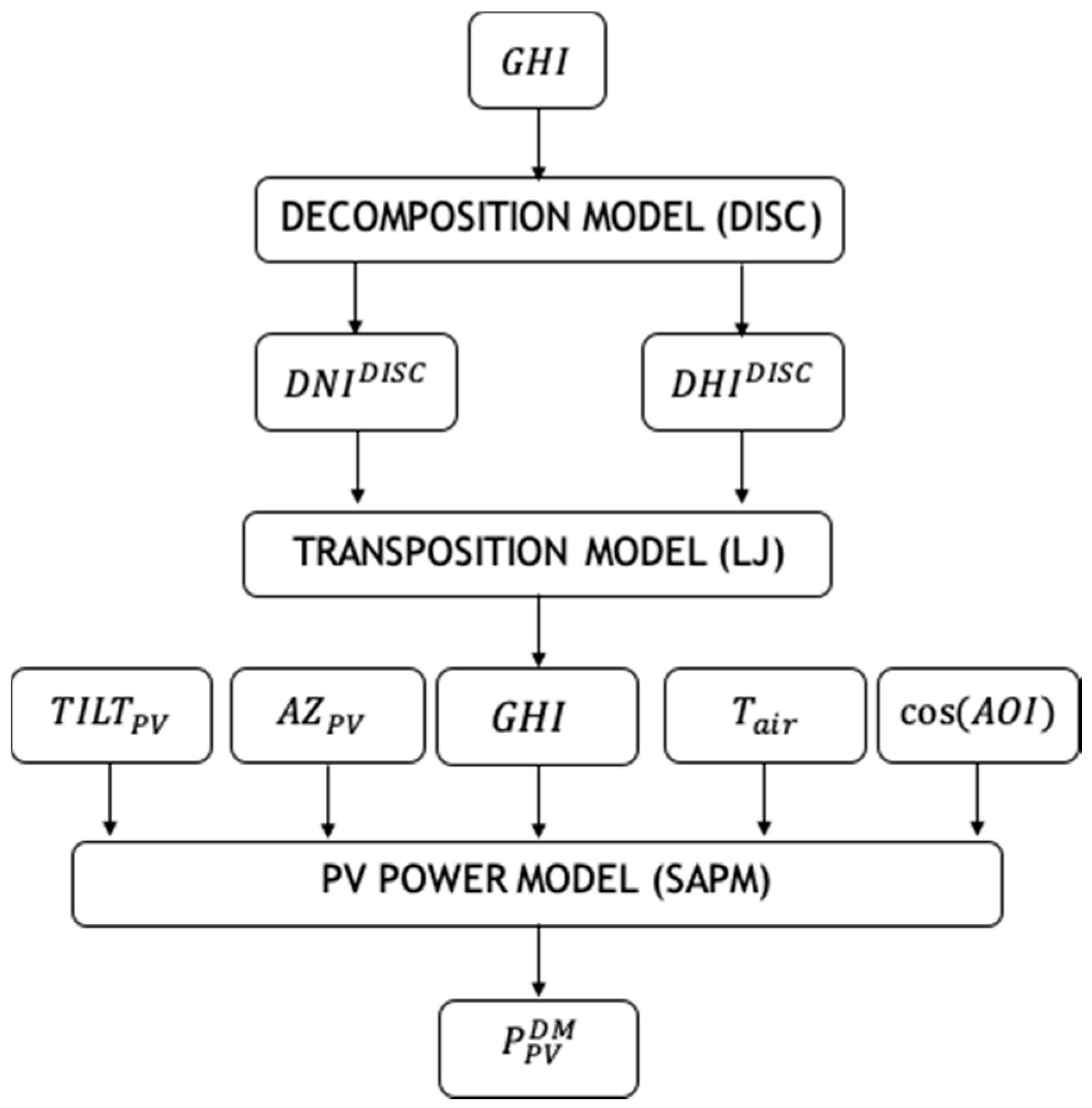
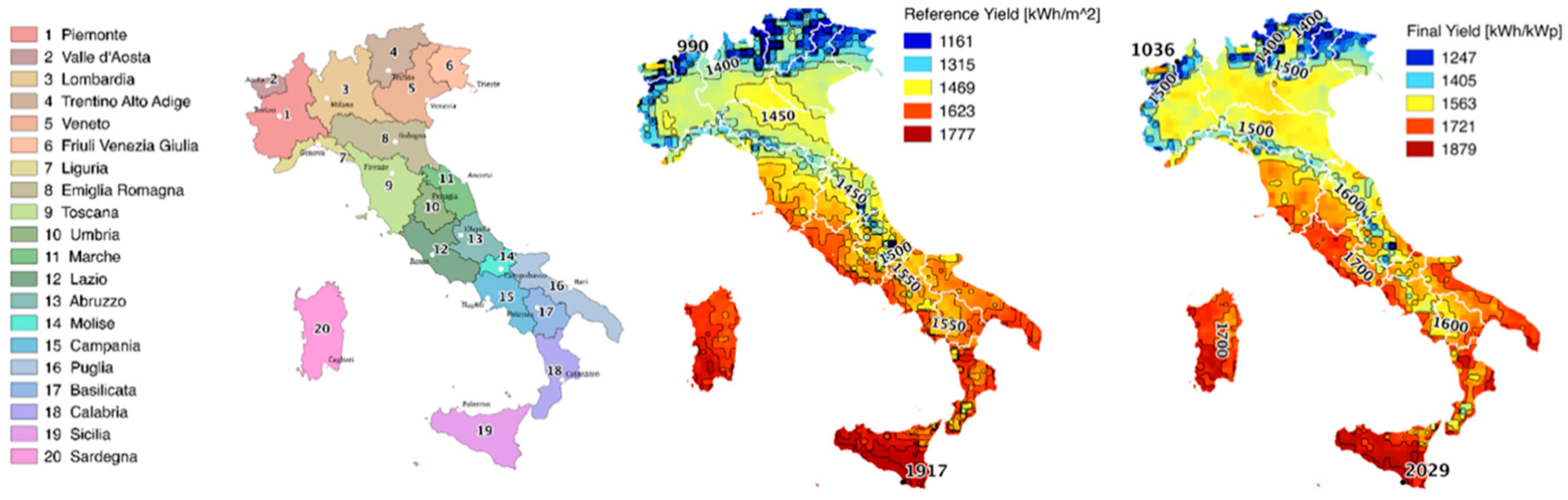
  • We mapped the satellite and the NWP irradiance into the generation of nominal PV plants placed on an optimal plane of array (30° tilted and south oriented) by a deterministic PV power method described in Section 4.1. The nominal PV production was simulated for each of the 1325 grid points covering Italy using four years of hourly data: 2014–2017 (see Figure 6b). The PV geometry was chosen taking into account that the “relevant” solar farms (PV systems with a capacity ≥10 MWp) are all optimally tilted and oriented.
  • We computed the energy imbalance between the current satellite derived PV generation and the day-ahead scheduled production for each point.
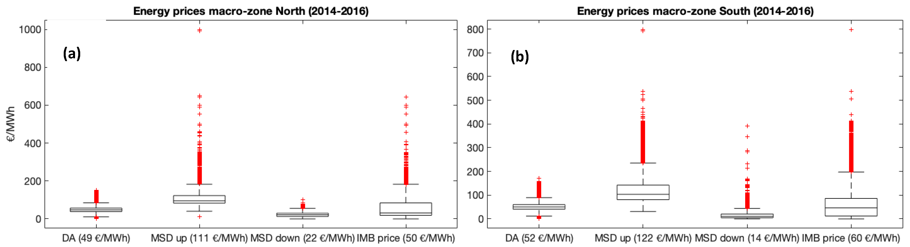
  • We evaluated the PV forecast economic value for each single “relevant” solar producer, by the DA and MSD ex-ante energy prices and the macro-zone imbalance signs related to the years 2014–2016. These energy price data were archived by Terna Spa, and are of public domain and downloadable from the TSO website [30].
To estimate and predict the PV generation of “relevant” solar farms, we used a deterministic “physical-based” method consisting of a chain of three semi-empirical models (Figure 8): (1) a decomposition model to retrieve the direct normal irradiance (DNI) and the diffuse irradiance (DHI) from the GHI data; (2) a transposition model to retrieve the global irradiance on the plane of array, i.e., the tilted irradiance (GTI); (3) a power estimation model to map the incident irradiance into PV generation.
The decomposition and the transposition models are the direct insolation simulation code (DISC) [31,32,33] and Liu–Jordan isotropic model (LJ) [34]. Both these semi-empirical methods are widely used since they need few number of inputs features. The first derives the DNI using only the global horizontal and the zenith angle [35], while the second needs only the DNI, DHI, and albedo to retrieve the GTI. The power estimation method is the Sandia Array Performance Model (SAPM) developed by King et al. at the Sandia laboratory [36]. This is one of the most accurate PV simulation models since it takes into account all the main effects that affect the PV performance in real operating conditions so that it can be used also for module performance characterization [37,38].
Therefore, the model inputs are the tilt and the orientation of the PV plant ( T I L T P V , A Z P V ) that in our case are 30° and 0° South, the GHI forecast ( G H I S A T   o r   G H I F O R ) , the air temperature forecast ( T a i r F O R ) and the angle of incidence (AOI) while the model output is the PV plant generation forecast per unit of the installed capacity ( P P V D M ) expressed in MW/MWp.
We compare the forecast accuracy and its economic value with those obtained by a simple persistence forecast (that is the reference model most used in the forecast literature):
P P V P ( h + H | d d ,   h ) = P P V ( h , d d )   w i t h   H = 24
where, d d is the current day and h is the hour of the day, P P V P is the simple persistence PV power forecast.

6. Metrics to Evaluate the Accuracy and Economic Imbalance Value

Table 2 reports two of the main metrics used in the forecast literature to evaluate the accuracy of non-probabilistic predictions, where X is the variable that should be predicted and n is the number of yearly sun hours.
The root mean square error (RMSE) accentuates the largest forecasting errors (i.e., outliers) while the skill score is exactly the accuracy improvement of the developed forecast method with respect to a baseline reference model (in our case, the persistence model). The RMSE is usually expressed in W/m2 in the case of irradiance or in MW or % of peak power in the case of a PV power forecast (since distribution system operator (DSO) and TSO usually adopt this unit), whereas the skill score (SS) is a dimensionless index.
The computation of the imbalance value for a single relevant solar plant has been explained in Section 3, and Table 2 also reports the main economic metrics. We mention that the net imbalance value ( N I V M S D ) is simply the hourly sum of the UP imbalance ( e h ( U P Z ) ) times the difference between the imbalance price on the MSD ex-ante ( V Z B ) and the energy price on the DA ( P Z D A ). It represents the value of the forecast with respect to the value of a “perfect” forecast, i.e., the total incomes of the MSD and DA achieved by the provided PV power forecast ( E I V D A & M S D f o r e c a s t ) net of the “ideal” incomes that could be achieved on the DA market with no imbalance ( E V D A ). In our case, the imbalance price ( V Z B ) is defined by the “single pricing” rule.

7. Results

7.1. Forecast Results

The observed 2014–2017 show horizontal radiation ranged from a minimum of 990 kWh/m2 in the North Alpine region to a maximum of 1900 kWh/m2 in the very South (Sicily). The country’s mean radiation was 1533 kWh/m2 per year (Figure 9).
It follows that the minimum Italian generation rate of “relevant” solar farms is around 1000 MWh/MWp in the North Alpine space, while the maximum is around 2000 MWh/MWp in the very South. The average generation rate of an optimal tilted and oriented PV system is around 1671 MWh/MWp (Figure 9).
Figure 10a reports the RMSE of our GHI forecast model plotted against the RMSE of the persistence model. Each point in this figure corresponds to one of the 1325 gridded locations. Our forecast errors range between 85.6 and 118.8 W/m2 depending on the location, while the persistence errors are between 131.7 and 179.2 W/m2. The skill score of the GHI forecasts range from 20% to 45%. Figure 10a also displays the error range of the day-ahead irradiance forecast benchmarks in four sites of four different EU countries, from five or four different forecasting methods, depending on location, Lorenz et al. [39]. The bars report the maximum, mean and minimum RMSE of the five/four day-ahead predictions in each EU site provided by the different forecasting methods. It is worth noting that our RMSE is near or below the fit of the best accuracy values obtained in the work of Lorenz et al. Our forecasts can be thus considered to be representative of “state of the art” forecasts. We also have to note that Lorenz et al. compared forecasts against ground measurements while here, we compare forecasts against satellite-retrieved irradiances. Nevertheless, it has been shown that satellite data are an acceptable, if not in many cases preferable, ground measurement proxy to both train and test forecast models [40,41,42,43,44].
Figure 10b plots the RMSE of our PV power forecast against the RMSE of the persistence, while Table 3 reports the accuracy of day-ahead forecasts of single plants’ generation in different countries.
Our forecast errors range between 11% and 16.7% of PV capacity (Pn), while the persistence errors are between 16.2 and 24.4% of Pn. Skill scores range from 25.7% to 39.7% with a mean value of 33.6%. Therefore, our accuracy benchmark is perfectly inside the range of accuracy reported in the literature.
We observe the highest regional RMSEs in Val d’Aosta, Liguria and Abruzzo, owing to the variable conditions due to the mountains. The lowest RMSEs are observed in the islands of Sardinia and Sicily (see Figure 11). The best skill scores occur in the north regions, Piemonte and Val d’Aosta, while the worst ones are observed in Abruzzo (due to the high weather variability) and in Puglia (due to highly persistent weather and the relatively good performance of persistence).
From the PV power forecasts at each of the 1325 Italian locations, we computed the annual imbalance costs/revenues for “relevant” PV producers or traders. We also computed the economic valorization of the forecast with respect to the persistence, i.e., the economic value of using predictions that are more accurate.
The benchmark of the imbalance economic value has been carried on using the years 2014–2016 according to the hourly DA and MSE ex-ante energy prices available on the Terna database (Figure 4).
Through this benchmark, we evaluate the effectiveness of the “single pricing” rule in promoting solar imbalance reduction, pointing out some important shortcomings of the Italian regulatory framework.

7.2. Benchmarking the Economic Value of the Imbalance of “Relevant” PV Plants

Figure 12a shows the imbalance valorization of the MSD in different locations/years using our deterministic PV generation forecast. As reported in Section 3, the “single pricing” rule can produce, for “relevant” PV production units, positive (revenues) or negative (costs) imbalance values that, in this case, range from 5 to −5 kEUR per MWp of PV capacity per year. There is a notable difference between the imbalances values obtained in different years. During 2014 and 2016, for the majority of the locations of the North, the imbalance is a cost (regions from 1 to 12), while in the South, it is mainly profit (regions from 13 to 20). In 2015, however, an energy imbalance generated a revenue almost everywhere in Italy.
Figure 12b shows the total energy incomes (on the DA and MSD markets) for “relevant” PV producers in different locations/years. These incomes range from 50 to 150 EUR/MWp per year and in this case, the higher incomes were obtained during the year 2015 with the only exception of Sicily.
Indeed, in Sicily, during the year 2014, the zonal energy market was affected by a high speculation level due to the grid bottleneck that does not allow the flow of additional cheaper power from the land. In addition, the “single pricing” market rule provides penalties/premium for solar imbalances according to the imbalance sign of the macro-zones in which the PV production unit is located. Therefore, as we will show later, energy traders can predict the imbalance macro-zonal sign to maximize their profits on the MSD market. Up to 2014, Sicily was itself a macro-zone, so that local PV producers could easily predict the macro-zonal imbalance sign increasing their profits also on the MSD. In order to reduce these trading speculations, after 2014, Terna improved the grid connection between the island and the land and incorporated Sicily and Sardinia into the South macro-zone, increasing difficulties in the prediction of the macro-zonal imbalances.
Figure 13 reports the yearly average (weighted with the corresponding exchanged energy) of the imbalance values on the MSD and of the energy trading values on the DA and MSD markets, per unit of produced energy. The average imbalance values range between −5 and 5 EUR/MWh, while the total values on the energy markets range between 37.5 and 80 EUR/MWh. Therefore, thanks to the “single pricing” system, the solar imbalance unitary values are more than ten times lower than the total trading values.
The annual economic loss/gain due to the errors in the PV generation scheduling is the value of the PV forecast, i.e., the net imbalance value (Table 2), and it can be computed as the difference between the total energy incomes on DA–MSD markets, and the energy revenues that could be realized with a perfect forecast (no imbalance).
The net imbalance values are costs in all the Italian regions with the exception of Lazio, Campania, Calabria and Sardinia, where there are some locations in which the imbalance could even make profits (Figure 14a).
The maximum economic losses are in the North zone with a zonal average of −2.8 kEUR/MWp and a range of −4.9 to −0.7 kEUR/MWp, while the minimum losses are in Sardinia with a zonal average of −0.6 kEUR/MWp and a range of −1.7 to 0.5 kEUR/MWp (Figure 14b).
Antonanzas et al. in [21] found a net imbalance value of a single plant on the Iberian energy markets under the “dual pricing” mechanism, which ranges between −2.6 and −3.3 kEUR/MWp depending on the forecast accuracy.
It is worth noting that the net imbalance values should always be a cost (negative), but there are some locations in which it is a revenue (positive) therefore, with the “single pricing” rule, an imperfect forecast could be more profitable than “perfect” forecasts. Moreover, the net imbalance values (that range between −5 and 0.6 kEUR/MWp), are quite small if compared with the total energy incomes (that range between 50 and 150 kEUR/MWp—Figure 12b), hence, with the “single pricing” rule, the imbalances have a small impact on the total energy revenues of PV producers.
From Figure 15a it can be observed that the imbalance values obtained using our forecast method (DM) are almost higher everywhere than the ones obtained using the persistence predictions (average of the years 2014–2016). In particular, the persistence predictions lead always to negative values, i.e., economic losses for producers.
The economic gains of the DM forecast with respect to the persistence on MSD can be computed as:
G a i n s M S D ( D M , P ) = {   | E I V M S D P | | E I V M S D D M |   i f   s i g n ( E I V M S D P E I V M S D D M ) > 0     | E I V M S D P | + | E I V M S D D M |   i f   E I V M S D P < 0   a n d   E I V M S D D M > 0 ( | E I V M S D P | + | E I V M S D D M | )   i f   E I V M S D P > 0   a n d   E I V M S D D M < 0 ,
where E I V M S D P and E I V M S D D M are the energy imbalance value produced by the persistence and the DM forecast.
Figure 15b shows that the mean regional imbalance gains are positive in all the regions and the increase in the forecast accuracy could produce benefits that range from 1 to 6 kEUR per MWp of PV capacity per year. This is considerably more than the cost of a high quality solar generation forecast.
The annual day-ahead market gains of our forecast (DM) with respect to persistence (P) can be computed as follows:
G a i n s D A ( D M , P ) = E V D A D M E V D A P = ( E V D A E V D A P ) ( E V D A E V D A D M ) = [ h = 1 n P Z D A ( h )   e h P ( U P ) ] [ h = 1 n P Z D A ( h )   e h D M ( U P ) ] ,
where E V D A D M and E V D A P are the annual energy values on the DA market obtained by the DM and persistence scheduling (Figure 16b), P Z D A is the energy price on the day-ahead market and e h D M , e h P are the prediction imbalances (Table 2).
It is worth noting that: h = 1 n P Z D A ( h )   e h P ( U P ) is always very small since persistence forecasts are almost always unbiased ( h = 1 n e h P ( U P ) 0 ) so that, when our DM forecast model provides an annual underprediction ( h = 1 n e h D M ( U P ) > 0 ) , there will be an high probability that the day-ahead market gains will be negative while, when the model provides an overprediction ( h = 1 n e h D M ( U P ) < 0 ) , the gains are likely to be positive. In this case, since our model provides a slight underprediction almost everywhere (Figure 17) the DA gains are mainly negative, ranging between −4.5 and 0.5 kEUR per MWp (Figure 16b). Therefore, our forecasts produce economic losses on the DA market with respect to the trivial persistence predictions.
It has to be pointed out that an under-forecast produces a lower income on the DA market but a higher/lower revenue/cost on the MSD since it mainly implies energy exchanges for downward regulations (at lowest dispatching prices) and vice versa.
Figure 18 summarizes all the results, reporting the total gains on both the DA and MSD markets obtained by our accurate forecast with respect to the persistence, i.e., the value of the accuracy improvement:
G a i n s D A & M S D ( D M , P ) = E V D A & M S D D M E V D A & M S D P ,
where E V D A & M S D D M and E V D A & M S D P are the annual energy incomes on the DA and MSD markets obtained by the DM and persistence forecasts.
Figure 18a shows that the economic gains of a DM forecast on the MSD market ( G a i n s M S D ( D M , P ) ) are positive almost everywhere in Italy (since our forecast is more accurate than the persistence prediction), while the gains on the DA market ( G a i n s D A ( D M , P ) ) are negative (since our forecast is slightly negative biased while persistence is almost unbiased). As a result, the total gains are strongly reduced or even cancelled out. A small benefit from using a more accurate forecast can be obtained in the North (NORD), Centre-South (CSUD), South (SUD) and Sicily (SICI) regions with average zonal values of 1.1, 0.4, 1.6 and 0.3 kEUR/MWp per year (Figure 18b). In contrast, negative gains appear in the Centre-North and Sardinia with average zonal values of −0.5 and −0.3 kEUR/MWp per year, hence, from an economic point of view, in these zones the persistence model should be preferred to our more accurate forecasting method.
The “single pricing” system not only allows revenues from solar imbalances reducing the net imbalance values of the forecast, but also reduces or cancels the economic benefits of using a more accurate forecast instead of the simple persistence prediction.
When the forecasts are show a low bias, it is much more difficult to obtain this paradoxical result when the “dual pricing” system is used since no revenues can be achieved on the MSD. Nicolas Ibagon et al. [22] showed that the imbalance costs resulting from the “dual pricing” are almost twice as large as costs resulting from the “single pricing” rule. Antonanzas et al. in [21] found a value of the forecast improvement with respect to persistence between 0.46 and 1.2 kEUR/MWp, depending on the forecast accuracy. Nevertheless, the authors still found that a less accurate forecast could produce higher benefits than more accurate ones. For this reason, they stated that the standard error metrics are not sufficient to evaluate the economic impact of the forecast. We add that this discrepancy between the accuracy and economic metrics is due to the dependence of the imbalance value on stochastic variables, the zonal imbalance sign and upward and downward regulation prices. Indeed, using both “single” and “dual” pricing rules, it is always possible that a poor forecast but with imbalances frequently in favor of the system (negative match between the zonal and UP imbalance signs) produces lower imbalance costs than a better forecast but with an imbalance frequently against the system (positive match between the imbalance signs). Therefore, as we will demonstrate in the next section, in order to reward the better forecasts, the market rules to compute the imbalance values should not depend anymore on these random variables.
We further point out another important shortcoming of the current imbalance market regulatory framework. The “single pricing” system produces a negative imbalance valorization (penalty) if the signs of the imbalances of the solar production unit (UP) and of the macro-zone (in which the UP is located) are the same, and the positive valorization (premium) if the UP and macro-zone imbalance signs do not match. Indeed, the incorrect solar generation scheduling, in the first case, increases the zonal imbalance while in the second case, helps to reduce the imbalance of the macro-zone. Even if this rule appears reasonable, it leads to another counterproductive effect regarding the need to reduce the imbalance volumes.
The imbalance values on the MSD ( E I V M S D f o r e c a s t ) can be decomposed in two factors:
E I V M S D f o r e c a s t = V Z   B A E I ,
where V Z   B is the average imbalance unitary value (EUR/MWh) and A E I is the imbalance volume (MWh/MWp per year), i.e., the accuracy of the forecast.
The value V Z   B embeds both the MSD energy prices (for upward or downward regulation) and the match between the UP and the macro-zonal imbalance signs.
Figure 19 shows that the imbalance values on the MSD market are much more correlated with the average imbalance unitary values than with the imbalance volumes.
This means that, for energy producers/traders under the “single price” rule, it is much more important to predict the right sign of the macro-zone imbalance and thus to provide Terna an adequate under/over-forecast rather than to deliver the most accurate forecast minimizing the volume of solar imbalance. In 2014, for this reason, the Italian TSO enlarged the size of the imbalance zones passing from four macro-zones to the current two. In this way, Terna increased the difficulties in predicting the macro-zonal sign, reducing the arbitrage activities on the imbalance market (see the imbalance valorization in Sicily during 2014 reported in Figure 13).
In contrast, Antonanzas et al. in [21] demonstrated that this kind of market speculation and these fraudulent activities are strongly limited by the “dual pricing”. They showed that there is a much higher correlation between the imbalance values and the imbalance volume with a well-fitted linear relation between these two quantities. Nevertheless, a small deviation from linearity can still give rise to lower economic benefits of the outperforming forecast (as previously discussed).
Clo and Fumagalli [26], in their study on the Italian shift of the settlement rules of consumption sites from a “single” to a “dual” pricing scheme, arrived at the same conclusion on the effectiveness of “dual pricing” in reducing the system imbalances.
From Figure 19, it is also worth noting that our DM forecasts not only provides a lower imbalance volume with respect to persistence, but also a higher average imbalance unitary values, i.e., a more profitable match between the UP and macro-zonal imbalance signs.
This could indicate that the majority of the solar producers use the persistence model to predict their PV generation. Indeed, for instance, if the majority of the “relevant” PV producers inside a macro-zone delivers a persistence over-forecast of their solar generation, Terna will predict a lower generation supply than needed; hence, there will be a negative imbalance of the macro-zone. At the same time, if a PV producer that, using another forecast model (for example our DM method), provided to Terna an under-forecast, it would supply more solar energy than expected, thus helping Terna to reduce the zonal imbalance. Therefore, this PV producer will have an economic premium while all the others will pay penalties for their imbalances. If this situation occurs many times during a year, it will result in a higher average imbalance unitary value for the producer that uses state of the art forecasts than for all the others that use the persistence prediction. In other words, as stated in [48], the forecasts with lower correlations with the TSO prediction (driven by the forecast of all the market agents) would have a higher probability of being in favor with the needs of the system and thus, to avoid penalties or earn rewards.
It is important to understand that the increase in the average imbalance unitary values depends only on the sign of the forecast error generated by one model (for instance our method) with respect to the imbalance sign obtained by the most used prediction model (the persistence model in this case), independently from the imbalance volumes that they generate with their predictions, i.e., from the forecast accuracy.

8. Proposed Revision to the Dispatching Market Regulatory Framework

The “single pricing” rule was introduced to reduce the imbalance penalties for variable renewable energy plants characterized by an unprogrammable generation. Nowadays, PV generation has reached grid parity. It is the cheapest source of electrical energy (at least on an unconstrained kWh basis) [1]. Therefore, the rule to compute the imbalance prices should be appropriately revised for all the new plants coming online to avoid the undesired effects mentioned above.
The simplest rule revision could be to shift from the “single” to the “dual” pricing schemes so that, as was demonstrated in [21,26], the best forecasts would be more probably rewarded and the market arbitrage actions would be strongly reduced.
However, we suggest a more radical regulatory reform.
First, we showed in [14] that solar imbalances can be halved just by operating proactive curtailment in all the case of under-forecasting, i.e., all the energy generated that exceeds the prediction is curtailed by smart inverters and control systems so that the grid injection will be the scheduled value.
The energy that should be curtailed is exactly the energy imbalance:
e h ( U P ) = E g e n e r a t i o n r e a l E g e n e r a t i o n f o r e c a s t = E g e n e r a t i o n f o r e c a s t + E g e n e r a t i o n c u r t a i m e n t E g e n e r a t i o n forecast = E generation curtaiment
The costs for the producers of the curtailed energy is exactly equal to the net imbalance costs, regardless of the market-pricing rule. Therefore, for the producers, it is economically the same to pay for the imbalance or to curtail the energy above the forecast (in effect, delivering a “perfect” forecast). Considering that all the new plants employ smart inverters, proactive curtailment should be mandatory. In this way, solar flexibility would be improved and the downward regulation due to solar-induced imbalance would be avoided.In addition, we suggest overcoming both the “single” and “dual” pricing mechanisms by removing any dependency from the zonal imbalance sign. The MSD imbalance price, in case of a negative imbalance (under-forecast), can be higher than the DA market price ( P Z D A ) by a fixed daily amount: ( Δ P Z B ( d ) = P Z B ( h ) P Z D A ( h ) d ) and the imbalance value can be calculated as: V Z B ( h ) = P Z D A ( h ) + Δ P Z B . The additional price Δ P Z B ( d ) on the MSD is the daily mean (sun hour only) of the differences between the zonal upward regulation price and the day-ahead price (computed ex-post).
With this simple rule change and proactive curtailment in case of an over-forecast, not only would the daily net imbalance value always be negative (i.e., a cost for the plant owners) but also it would be directly proportional to the daily upward imbalance volumes. Indeed, the daily net imbalance value would become:
N I V ( d ) = h = 1 24 ( V Z B ( h ) P Z D A ( h ) )   e h ( U P ) = Δ P Z B ( d ) h = 1 n u p   | e h ( U P ) | ,
where n _ u p is the number of hours of the day ( d ) during which the plant generated less than scheduled (negative imbalance).
The imbalance costs for the producers would be higher than the one obtained by the “dual” pricing scheme, in case of an upward regulation, since they would pay for the under-scheduling regardless of the zonal imbalance sign. To reduce these penalties, the producers could either improve their forecasts or use systematic under-forecasts and over-curtail. In both these cases, it would result in a lower solar-induced imbalance.
With this pricing scheme, the most appropriate physical metric to assess the forecast quality becomes the yearly average of the daily mean absolute imbalance errors:
M A E ( d ) y e a r = 1 n _ u p h = 1 n _ u p   | e h ( U P ) | y e a r ,
Nevertheless, there remains a discrepancy between the economic metric, N I V ( d ) y e a r , and the physical metric, M A E ( d ) y e a r , induced by the stochastic variability of the daily additional prices, Δ P Z B ( d ) . However, at a high solar penetration, higher MSD additional prices Δ P Z B ( d ) would naturally appear during days with irradiance that is more difficult to predict. Therefore, the forecasts with lower M A E ( d ) y e a r will most likely produce the lowest annual imbalance costs ( N I V ( d ) y e a r ) . In addition, any market arbitrage based on the forecasting of the zonal imbalance sign would be eliminated.
It is worth recalling that full solar flexibility could be reached by equipping the PV systems with battery energy storage systems (BESS) so that they can provide not only a proactive curtailment in case of an under-forecast, but also an additional power supply in case of an over-forecast. This kind of system we called “flexible” PV plants, and they are able to reduce their imbalance as well as to eventually provide a perfect predictable generation [14].
In [14], we also proved that the solar-induced imbalance of the whole Italian PV fleet can be limited by the use of “relevant” and “flexible” solar plants that provide ancillary services. The costs of this solar regulation can be lower than the current imbalance costs if these flexible plants are under the control of the Italian TSO that uses them to correct the forecast error of the whole Italian generation. Thus, we suggest to economically support solar producers that install such flexible plants leaving their control to the national TSO. This support could consist of paying for all the generated energy and the additional BESS power at day-ahead market prices, adding a suitable amount to pay back the BESS’ capital and operating costs (CapEx and OpEx). In this way, producers would maximize their revenues (since no imbalance cost would be charged) and improve the value of their plants with full flexibility without additional cost for BESS installation and O&M. As we showed in [14], this economic incentive for flexible PV farms employed for solar regulation could be paid for by the saving in national imbalance costs.
In [50], we further show applying solar regulation to the forecast certainty is the first logistical step to gradually reach an ultra-high PV penetration in Italy (achieving over 92% of RE energy contribution).

9. Conclusions

We first showed that the accuracy of our irradiance forecasts could be considered “state of the art” in Italy. We then applied a deterministic method to convert the predicted irradiances into PV production from optimally oriented and tilted solar plants. We thus provided a benchmark for the forecast accuracy of the “relevant” PV plants generation in 1325 locations in Italy. We found that the RMSE of the day-ahead predictions ranged from 12% and 16% of the PV nominal capacity, with a skill score ranging between 25% and 40% depending on the location.
We used the PV power forecast results to provide a benchmark for the net imbalance values of “relevant” PV plants, i.e., the energy values on the DA and MSD markets ideal incomes that could be obtained on the DA market with no imbalance (i.e., perfect forecast). We found these values to be mainly negative (economic losses) and, for the regional average, decreasing from the North to the South of the country, passing from −2.8 kEUR/MWp to −0.6 kEUR/MWp.
We also compared the energy values on the MSD and DA markets that could be achieved by the use of our forecasts to the energy values obtainable by a simple persistence prediction. Almost everywhere in the country our forecast produces lower economic losses or higher revenues than persistence methods for the MSD market place. The benefits of our forecast, with respect to the persistence prediction, ranges from 1 to 6 kEUR per MW of PV capacity per year. This is considerably more than the cost of high quality solar power forecasts. Nevertheless, we showed that these benefits were strongly reduced or even cancelled if we also considered the energy incomes obtainable by the PV generation scheduling on the DA market. Indeed, in some regions, the persistence prediction could produce even more profits than a much more accurate forecast for the DA and MSD markets.
We highlighted several important shortcomings of the Italian “single pricing” system that brings paradoxical and counterproductive effects regarding the need to reduce the solar-induced imbalance volumes.
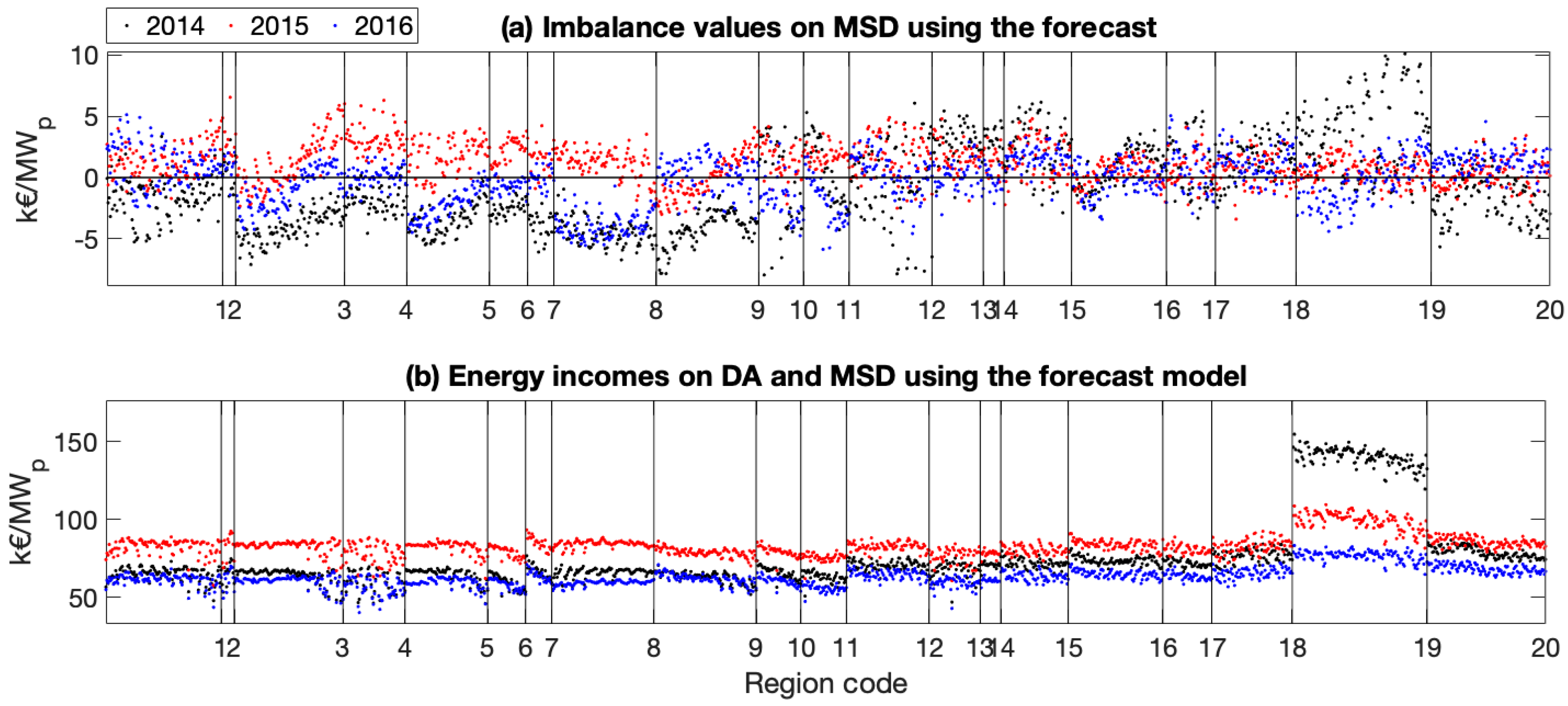
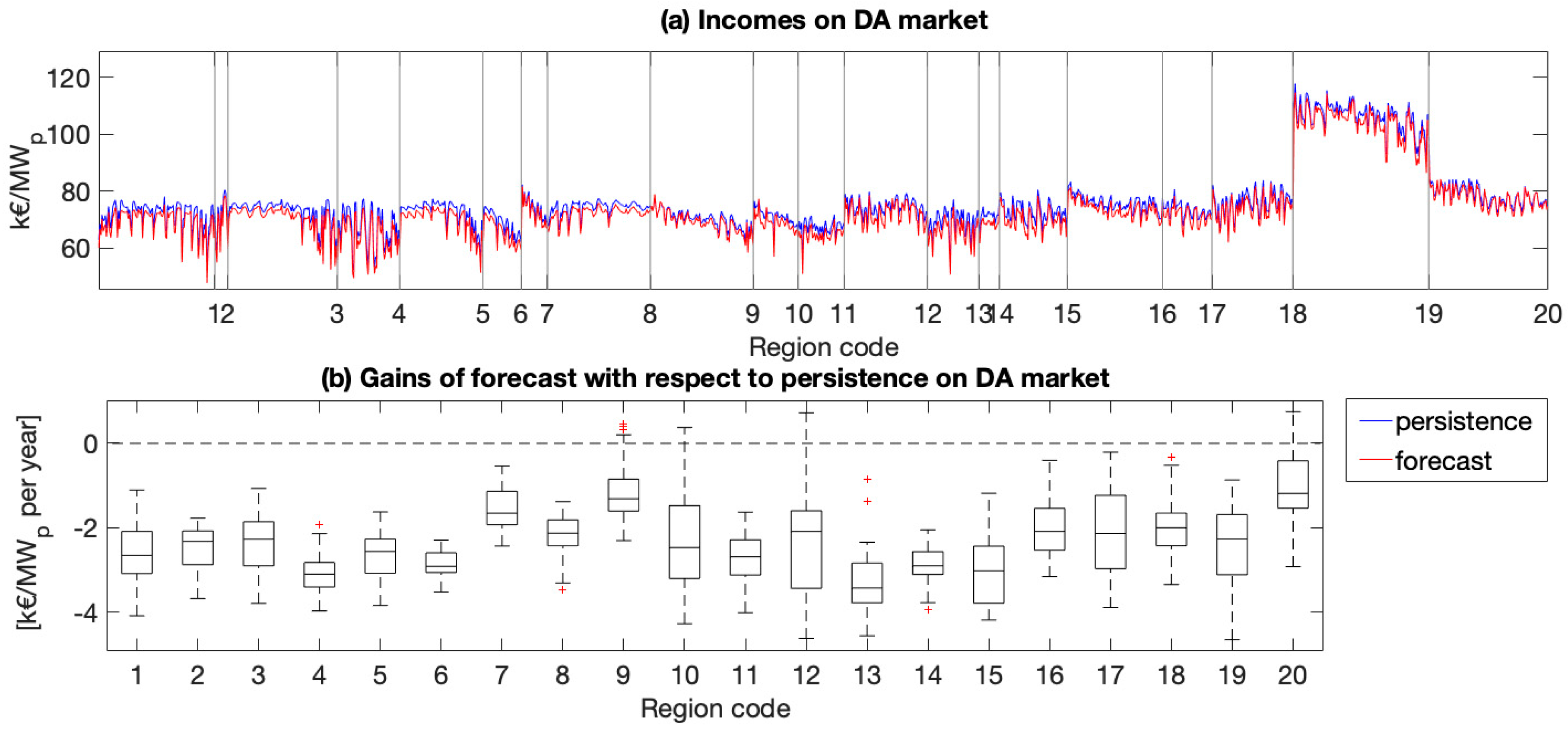
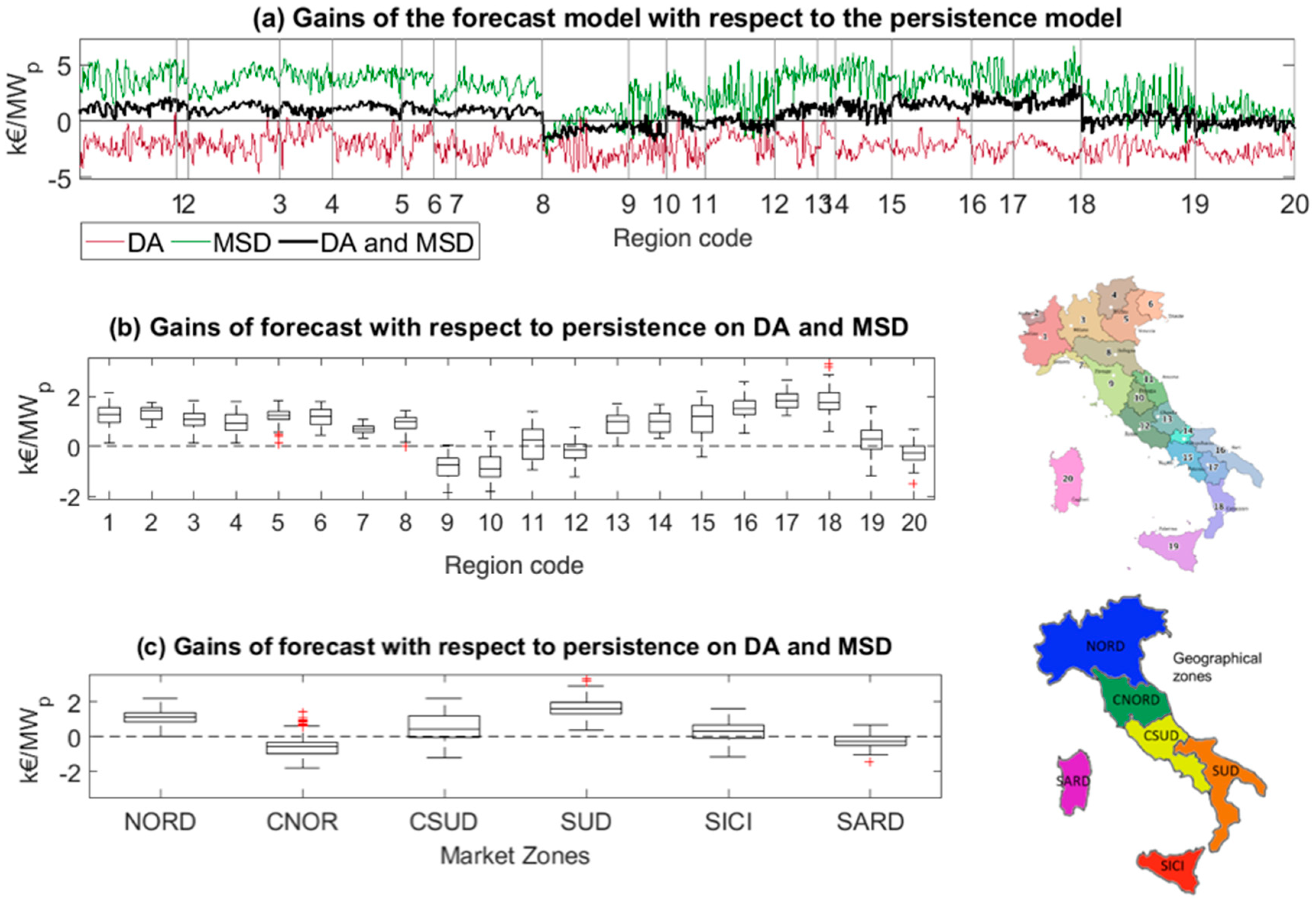
  • The net imbalance absolute values (that ranges from −5 to 5 kEUR/MWp per year) are very small if compared with the total energy incomes on the DA and MSD markets (that ranges from 50 to 150 kEUR/MWp per year) hence, with the current market rules, the imbalances have a small impact on the total energy revenues of the PV producers/traders.
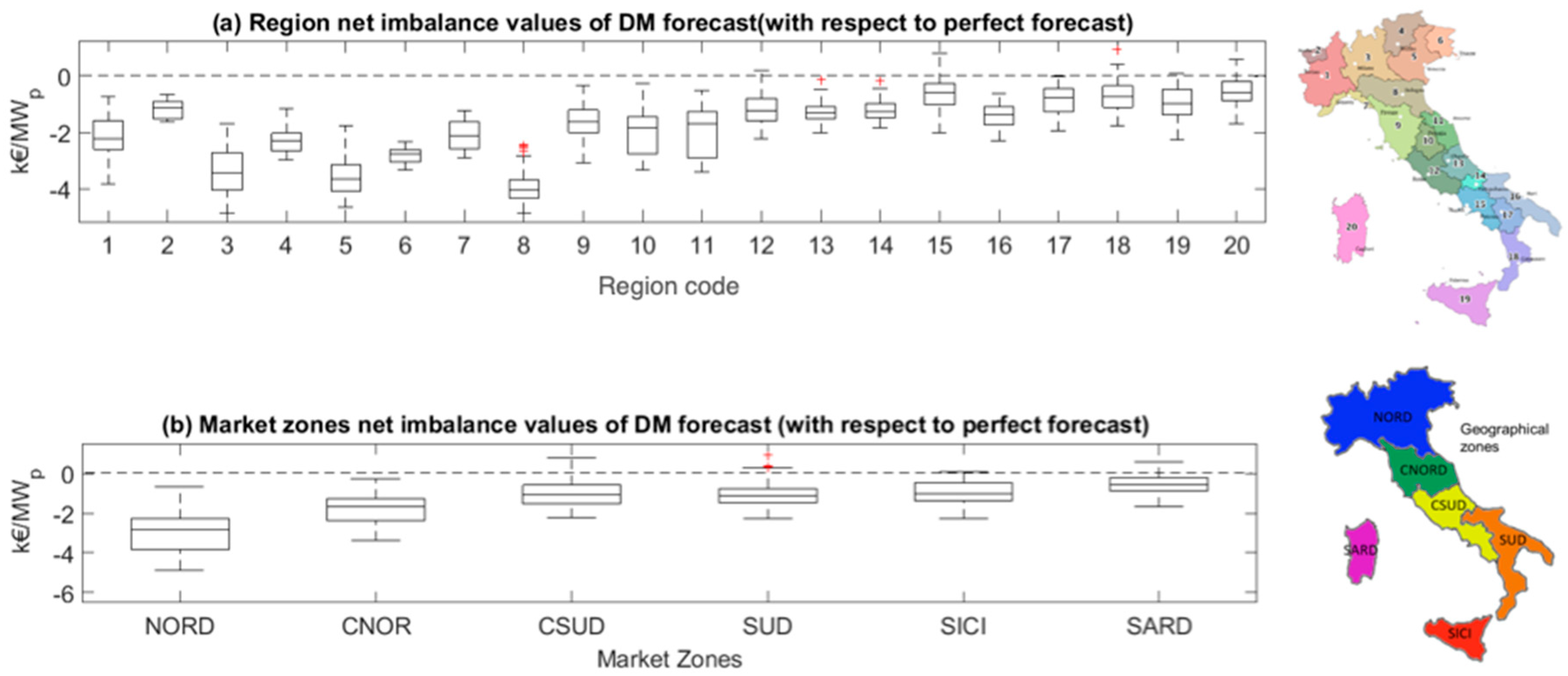
  • The net imbalance values that should be always negative (economic losses for producers) in some locations can be also positive (economic revenues). Hence, a poorly predicted PV generation could even lead to higher profits than an “ideal” perfectly predictable generation (that will not produce a solar-induced imbalance).
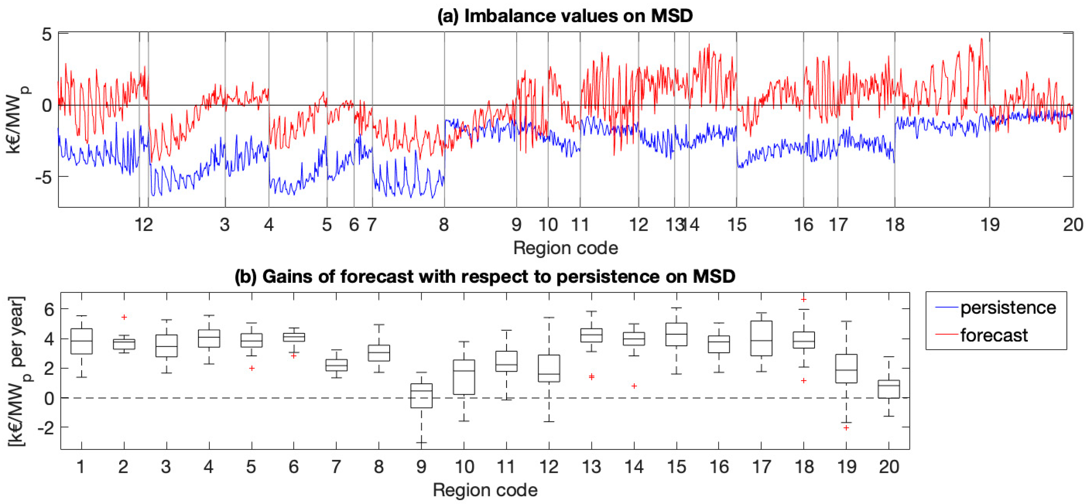
  • Not only is the benefit of using a more accurate forecast with respect to a simple persistence very small, but in some regions persistence predictions produce even higher revenues. Therefore, in these regions, there is no economic need to improve the forecast accuracy reducing the solar imbalance volumes.
  • For energy producer/traders, it is much more important, in order to maximize revenues, to predict the right macro-zonal imbalance sign and then deliver to Terna a suitable under/over PV generation forecast than provide Terna with the most accurate power prediction.
  • Therefore, we demonstrated that, in Italy, the current market regulation framework is in complete disagreement with the physical need of reducing imbalances and hence it requires a significant revision to allow a higher PV penetration.
Finally, we suggested a simple revision of dispatching market regulatory frameworks that would avoid all the undesired effects of the “single pricing” scheme, forcing the solar producers to be balanced.

Author Contributions

Conceptualization, M.P. and R.P.; Data curation, M.P.; Funding acquisition, D.M.; Supervision, D.M., R.P. and C.C.; Writing—original draft, M.P.; Writing—review and editing, D.M., R.P. and C.C. All authors have read and agreed to the published version of the manuscript.

Funding

This research was supported by the Province of Südtirol, ERDF Project, INTEGRIDS FESR1042.

Acknowledgments

Marco Pierro thanks the Institute for Renewable Energy, Eurac Research, Bolzano, Italy for supporting his Ph.D. A special thank you to the forecast provider IDEAM S.r.l. that supplied the satellite and NWP data for this work.

Conflicts of Interest

The authors declare no conflict of interest.

References

  1. Ministry of Environment. SEN (Strategia Energetica Nazionale); Ministry of Environment: Rome, Italy, 2017.
  2. Proposta dI Piano Nazionale Integrato per l’Energia e il Clima. Available online: https://www.mise.gov.it/images/stories/documenti/Proposta_di_Piano_Nazionale_Integrato_per_Energia_e_il_Clima_Italiano.pdf (accessed on 1 December 2019).
  3. Sandbag, D.; Agora Energiewende. The European Power Sector in 2018. Up-to-Date Analysis on the Electricity Transition; Agora Energiewende: Berlin, Germany, 2019. [Google Scholar]
  4. IEA. Trends 2018 in Photovoltaic Applications. 2018. Available online: http://www.iea-pvps.org/fileadmin/dam/intranet/task1/IEA_PVPS_Trends_2018_in_Photovoltaic_Applications.pdf (accessed on 1 August 2020).
  5. ISPRA. Fattori di Emissione di Gas Serra e Altri Gas Nel Settore Elettrico 280/2018; ISPRA: Rome, Italy, 2018.
  6. Terna Spa. Il Mercato per il Servizi di Dispacciamento (Seminario RSE). 17 October 2016. Available online: www.rse-web.it/commons/layout/partUploaderView.jsp?CM=FILEVIEW&FILE_TO_UPLOAD=WF_3323_Terna+-+SEMINARIO+RSE_MSD_20161017.pdf%2B%2B%2Bapplications%5Cwebwork%5Csite_rse%5Clocal%5Cdocument%2F003323.Terna+-+SEMINARIO+RSE_MSD_20161017.pdf&TREATASATTACH=yes (accessed on 1 August 2020).
  7. Terna Spa. Methodologia di Previsione della Domanda Elettrica e della Previsione da Fonti Rinnovabili ai Fini della Dase di Programmazione di MSD; Terna Spa: Rome, Italy, 2016. [Google Scholar]
  8. Zhang, J.; Hodge, B.; Lu, S.; Hamann, H.; Lehman, B. Baseline and target values for regional and point PV power forecasts: Toward improved solar forecasting. Sol. Energy 2015, 122, 804–819. [Google Scholar] [CrossRef] [Green Version]
  9. Martinez-Anido, C.B.; Botor, B.; Florita, A.; Draxl, C.; Lu, S.; Hamann, H.; Hodge, B. The value of day-ahead solar power forecasting improvement. Sol. Energy 2016, 129, 192–203. [Google Scholar] [CrossRef] [Green Version]
  10. Wu, J.; Botterud, A.; Mills, A.; Zhou, Z.; Hodge, B.; Heaney, M. Integrating solar PV (photovoltaics) in utility system operations: Analytical framework and Arizona case study. Energy 2015, 85, 1–9. [Google Scholar] [CrossRef] [Green Version]
  11. Joos, M.S. Short-term integration costs of variable renewable energy: Wind curtailment and balancing in Britain and Germany. Renew. Sustain. Energy Rev. 2018, 86, 45–65. [Google Scholar] [CrossRef]
  12. Pierro, M.; De Felice, M.; Maggioni, E.; Moser, D.; Perotto, A.; Spada, F.; Cornaro, C. Photovoltaic generation forecast for power transmission scheduling: A real case study. Sol. Energy 2018, 174, 976–990. [Google Scholar] [CrossRef]
  13. Pierro, M.; De Felice, M.; Maggioni, E.; Moser, D.; Perotto, A.; Spada, F.; Cornaro, C. Residual load probabilistic forecast for reserve assessment: A real case study. Renew. Energy 2020, 149, 508–522. [Google Scholar] [CrossRef]
  14. Pierro, M.; Perez, R.; Perez, M.; Moser, D.; Cornaro, C. Italian protocol for massive solar integration: Imbalance mitigation strategies. Renew. Energy 2020, 153, 725–739. [Google Scholar] [CrossRef]
  15. Perez, R.; Perez, M.; Pierro, M.; Kivalov, S.; Schlemmer, J.; Dise, J.; Keelin, P.; Grammatico, M.; Swierc, A.; Ferreira, J.; et al. Operationally perfect solar power forecasts: A scalable strategy to lowest-cost firm solar power generation. In Proceedings of the 46th IEEE PV Specialists Conference, Chicago, IL, USA, 16–21 June 2019. [Google Scholar]
  16. Perez, M.; Perez, R.; Rábago, K.; Putnam, M. Overbuilding & curtailment: The cost-effective enablers of firm PV generation. Sol. Energy 2019, 180, 412–422. [Google Scholar]
  17. Gari da Silva Fonseca, J., Jr.; Nishitsuji, Y.; Udagawa, Y.; Oozeki, T. Improving regional PV power curtailment with better day-ahead PV forecasts: An evaluation of 3 forecasts. In Proceedings of the IEEE 7th World Conference on Photovoltaic Energy Conversion (WCPEC), Waikola, HI, USA, 10–15 June 2018. [Google Scholar]
  18. Kaur, A.; Nonnenmacher, L.; Pedro, H.; Coimbra, C. Benefits of solar forecasting for energy imbalance markets. Renew. Energy 2016, 86, 819–830. [Google Scholar] [CrossRef]
  19. De Giorgi, M.; Congedo, P.; Malvoni, M.; Laforgia, D. Error analysis of hybrid photovoltaic power forecasting models: A case study of mediterranean climate. Energy Convers. Manag. 2015, 100, 117–130. [Google Scholar] [CrossRef]
  20. Bignucolo, F.; Raciti, A.; Rossi, B.; Zingales, A. Management of renewable generation plants: Imbalance costs and local storage systems. In Proceedings of the AEIT Annual Conference, Palermo, Italy, 3–5 October 2013. [Google Scholar]
  21. Antonanzas, J.; Pozo-Vázquez, D.; Fernandez-Jimenez, L.; Martinez-De-Pison, F.J. The value of day-ahead forecasting for photovoltaics in the Spanish electricity market. Sol. Energy 2017, 158, 140–146. [Google Scholar] [CrossRef]
  22. Ibagon, C.N.; Oliveri, V.; Delfanti, M. Analysis of European RES Imbalance Charge: THE impact on PV and Wind Plants. 2014. Available online: https://www.politesi.polimi.it/bitstream/10589/86586/3/2013_12_Ibagon.pdf (accessed on 1 August 2020).
  23. Terna Spa (92/2019). 2019. Available online: https://www.terna.it/it/sistema-elettrico/mercato-elettrico/zome-mercato (accessed on 1 August 2020).
  24. GME. 2019. Available online: http://www.mercatoelettrico.org/it/Mercati/MercatoElettrico/MPE.aspx (accessed on 1 August 2020).
  25. Terna Spa. Piano di Sviluppo 2019; Terna Spa: Rome, Italy, 2019. [Google Scholar]
  26. Clo’, S.; Fumagalli, E. The effect of price regulation on energy imbalances: A Difference in differences design. Energy Econ. 2019, 81, 754–764. [Google Scholar] [CrossRef]
  27. Skamarock, W.; Klemp, J.; Dudhia, J.; Gill, D.; Barker, D. A Description of the Advanced Research WRF Version 3. NCAR Tech; Note NCAR/TN-4751STR; Technical Report NCAR: Boulder, CO, USA, 2008. [Google Scholar]
  28. Houghton, J. The Physics of Atmospheres, 3rd ed.; Cambridge University Press: Cambridge, UK, 2002; p. 340. [Google Scholar]
  29. Pierro, M.; De Felice, M.; Maggioni, E.; Moser, D.; Perotto, A.; Spada, F.; Cornaro, C. Model output statistics cascade to improve day ahead solar irradiance forecast. Sol. Energy J. 2015, 117, 99–113. [Google Scholar] [CrossRef]
  30. Terna Spa. Available online: https://www.terna.it (accessed on 1 August 2020).
  31. Ineichen, P.; Perez, R.; Seal, R.; Zalenka, A. Dynamic global-to-direct irradiance conversion models. ASHRAE Trans. 1992, 98, 354–369. [Google Scholar]
  32. Perez, R.; Seals, R.; Zelenka, A.; Ineichen, P. Climatic evaluation of models that predict hourly direct irradiance from hourly global irradiance: Prospects for performance improvements. Sol. Energy 1990, 44, 99–108. [Google Scholar] [CrossRef] [Green Version]
  33. Marion, B. A model for deriving the direct normal and diffuse horizontal irradiance from the global tilted irradiance. Sol. Energy 2015, 122, 1037–1046. [Google Scholar] [CrossRef] [Green Version]
  34. Liu, B.; Jordan, R.C. Daily insolation on surfaces tilted towards equator. ASHRAE 1961, 10, 526–541. [Google Scholar]
  35. Maxwell, A.L. A Quasi-Physical Model for Converting Hourly Global Horizontal to Direct Normal Insolation; Technical Report SERI/TR-215-3087; Solar Energy Research Institute: Golden, CO, USA, 1987. [Google Scholar]
  36. King, D.; Kratochvil, J.; Boyson, W. Photovoltaic Array Performance Model; Sandia National Laboratories: Albuquerque, NM, USA, 2004. [Google Scholar]
  37. Pierro, M.; Bucci, F.; Cornaro, C. Full characterization of photovoltaic modules in real operating conditions: Theoretical model, measurement method and results. In Progress in Photovoltaics; Wiley Online Library: Hoboken, NJ, USA, 2015; Volume 23, pp. 443–461. [Google Scholar]
  38. Pierro, M.; Bucci, F.; Cornaro, C. Impact of light soaking and thermal annealing on amorphous silicon thin film performance. In Progress in Photovoltaics; Wiley Online Library: Hoboken, NJ, USA, 2015; Volume 23, pp. 1581–1596. [Google Scholar]
  39. Lorenz, E.; Remund, J.; Muller, S.C.; Traunmull, W.; Steinmaurer, G.; Pozo, D.; Ruiz-Arias, J.; Fanego, V.L.; Ramirez, L.; Romeo, M.G. Benchmarking of different approaches to forecast solar irradiance. In Proceedings of the 24th European Photovoltaic Solar Energy Conference, Hamburg, Germany, 21–25 September 2009. [Google Scholar]
  40. Perez, R.; Kivalov, S.; Schlemmer, J.; Hekmer, K., Jr.; Rene, D.; Hoff, T.E. Validation of short and medium term operational solar radiation forecasts in the US. Sol. Energy 2010, 84, 2161–2172. [Google Scholar] [CrossRef]
  41. Perez, R.; Schlemmer, J.; Kankiewicz, A.; Dise, J.; Tadese, A.; Hoff, T. Detecting calibration drift at ground truth stations a demonstration of satellite irradiance models’ accuracy. In Proceedings of the 2017 IEEE 44th Photovoltaic Specialist Conference (PVSC), Washington, DC, USA, 25–30 June 2017. [Google Scholar]
  42. Yang, D.; Perez, R. Can we gauge forecasts using satellite-derived solar irradiance? J. Renew. Sustain. Energy 2019, 11, 023704. [Google Scholar] [CrossRef]
  43. André, M.; Perez, R.; Soubdhan, T.; Schlemmer, J.; Calif, R.; Monjoly, S. Preliminary assessment of two spatio-temporal forecasting technics for hourly satellite-derived irradiance in a complex meteorological context. Sol. Energy 2019, 177, 703–712. [Google Scholar] [CrossRef]
  44. Palmer, D.; Koubli, E.; Cole, I.; Betts, T.; Gottschalg, R. Satellite or ground-based measurements for production of site specific T hourly irradiance data: Which is most accurate and where? Sol. Energy 2018, 165, 240–255. [Google Scholar] [CrossRef]
  45. Lorenz, E. PV Production Forecast of Balance Zones in Germany; PVPS Task 14 & SHC Task 46; IEA: Paris, France, 2015.
  46. Pelland, S.; Galanis, G.; Kallos, G. Solar and photovoltaic forecasting through post-processing of the Global Environmental Multiscale numerical weather prediction model. Prog. Photovolt Res. Appl. 2013, 21, 284–296. [Google Scholar] [CrossRef]
  47. Zamo, M.; Mestre, O.; Arbogast, P.; Pannekoucke, O. A benchmark of statistical regression methods for short-term forecasting of photovoltaic electricity production part I: Deterministic forecast of hourly production. Sol. Energy 2014, 115, 792–803. [Google Scholar] [CrossRef]
  48. Antonanzas, J.; Perpinan-Lamigueiro, O.; Urraca, R.; Antonanzas-Torresa, F. Influence of electricity market structures on deterministic solar forecasting verification. Sol. Energy 2020, in press. [Google Scholar] [CrossRef]
  49. Pierro, M.; Defelice, M.; Bucci, F.; Maggioni, E.; Moser, D.; Perotto, A.; Spada, F.; Cornaro, C. Multi-model ensemble for day ahead prediction of photovoltaic power generation. Sol. Energy 2016, 134, 132–146. [Google Scholar] [CrossRef]
  50. Pierro, M.; Perez, R.; Perez, M.; Moser, D.; Cornaro, C. Italian protocol for massive solar integration: From solar imbalance mitigation to 24/365 solar power generation. Renew. Energy 2020. under peer review. [Google Scholar]
Figure 1. Evolution and the Integrated National Plan for Energy and Climate (PNEC) scenario of the Italian energy mix (a); PNEC scenario for RES generation (b (elaboration from [2,5])).
Energies 13 03945 g001
Figure 2. Load, photovoltaic (PV) and wind day-ahead forecast errors and the resulting system imbalance during a day in August 2015 in Italy. Source: the Italian transmission system operator (TSO (Terna)) [6].
Energies 13 03945 g002
Figure 3. Spot markets in Italy.
Energies 13 03945 g003
Figure 4. Energy prices in the two macro-zones during the years 2014–2016: the DAM price ( P Z D A ), MSD prices for upward and downward regulations ( P Z B and P Z B ) and the imbalance price resulting from the “single pricing” rule ( V Z B ). In brackets are reported the average values. (a) North macro zone; (b) South macro zone.
Energies 13 03945 g004
Figure 5. Process to compute the solar production unit (UP) imbalance values.
Energies 13 03945 g005
Figure 6. Short wave radiation in the Weather Research and Forecasting model (WRF) model domain (a), 1325 irradiance satellite/forecast points computed on a grid of 12 × 12 km (b).
Energies 13 03945 g006
Figure 7. Methodology diagram.
Energies 13 03945 g007
Figure 8. Site PV power estimation/forecast method diagram.
Energies 13 03945 g008
Figure 9. Maps of Italy: Italian regions, reference yield (global horizontal annual radiation) and final yield (annual energy rate). The average values of the satellite derived radiation and power estimation over the years 2014–2017.
Energies 13 03945 g009
Figure 10. RMSE of the irradiance forecast vs. RMSE of persistence (average values over the years 2014–2017) and comparison with the forecasting errors resulting from different forecasting methods in four EU locations [39] (the dashed line is the fit of the accuracy of the outperforming forecasts (a)); RMSE of the PV power forecast vs. RMSE of persistence (b).
Energies 13 03945 g010
Figure 11. Regional RMSE and skill score of the PV generation forecast (averaged over the years 2014–2017).
Energies 13 03945 g011
Figure 12. Imbalance values on the MSD ex-ante resulting from the PV generation forecast model (a); energy incomes on the DA and MSD ex-ante resulting from the PV generation forecast (b). Positive value are revenues while negative are economic costs. Each point on the graphs is the annual energy value achievable in one of the 1325 locations (wider regions imply more points).
Energies 13 03945 g012
Figure 13. Yearly average imbalance values on the MSD ex-ante per unit of produced energy (a); yearly average trading values on the DA and MSD ex-ante (b).
Energies 13 03945 g013
Figure 14. Net imbalance values aggregated by the regions and market zones. (a) Region net imbalance values of DM forecast (with respect to perfect forecast). (b) Market zones net imbalance values of DM forecast (with respect to perfect forecast).
Energies 13 03945 g014
Figure 15. Imbalance values on MSD ex-ante per unit of PV capacity resulting from the use of the persistence and our forecast models (average 2014–2016 (a)); MSD ex-ante gains per unit of PV capacity resulting from the use of our PV generation forecast instead of the persistence prediction, aggregated by regions (b). Negative gains are losses.
Energies 13 03945 g015
Figure 16. Energy trading incomes on the DA market per unit of PV capacity resulting from the use of persistence and our forecast models (average 2014–2016) (a); gains on the DA market per unit of PV capacity resulting from the use of our PV generation forecast instead of the persistence prediction, aggregated by region (b). Negative gains are losses.
Energies 13 03945 g016
Figure 17. Frequency of the forecast mean bias errors. It has to be reminded that h = 1 n e h DM ( UP ) = n M B E .
Energies 13 03945 g017
Figure 18. Energy trading gains on the DA, MSD ex-ante and on both the markets per unit of PV capacity resulting from the use of our DM forecast instead of the persistence prediction (average 2014–2016 (a)); gains on the DA and MSD ex-ante per unit of PV capacity resulting from the use of our DM forecast instead of the persistence prediction, aggregated by the region and market zones (b,c). Negative gains are losses.
Energies 13 03945 g018
Figure 19. Scatter plot of the average imbalance unitary values on the MSD ex-ante vs. the imbalance values per unit of PV capacity (a); scatter plot of the imbalance volumes per unit of PV capacity vs. the imbalance values per unit of PV capacity (b).
Energies 13 03945 g019
Table 1. The balancing energy market (BEM) “single pricing” imbalance valorization scheme for the relevant production units not allowed to provide dispatching services ( P Z D A is the day-ahead market (DAM) zonal price; P Z B and P Z B are the market of the dispatching services (MSD) ex-ante purchase/sale zonal prices).
Energies 13 03945 i001Sign of the Imbalance of Relevant Production Unit (Market Zone Z)
Over generation with respect the day-ahead scheduling)Under generation with respect the day-ahead scheduling)
( E i m b M S D ( U P , h ) > 0 ( E i m b M S D ( U P , h ) < 0
(+)(−)
Sign of Macro-zonal ImbalanceOver generation(+)UP sells to TSO their imbalance at minimum MSD priceUP purchases from TSO their imbalance at minimum MSD price
V Z B = min { P Z D A , P Z B }. V Z B = min { P Z D A , P Z B }.
Negative imbalance value (cost)Positive imbalance value (revenue)
E i m b M S D ( U P , h ) ( V Z B P Z D A ) 0 E i m b M S D ( U P , h ) ( V Z B P Z D A ) 0
Under generation(−)UP sells to TSO their imbalance at maximum MSD priceUP purchases from TSO their imbalance at maximum MSD price
V Z B = max { P Z D A , P Z B } V Z B = max { P Z D A , P Z B }
Positive imbalance value (revenue)Negative imbalance value (cost)
E i m b M S D ( U P , h ) ( V Z B P Z D A ) 0 E i m b M S D ( U P , h ) ( V Z B P Z D A ) 0
Table 2. Metrics for the accuracy assessment and economic imbalance valorization.
NameAcronym and Formulae
Forecast error
[W/m2 or MW-% of peak power]
e h = ( X for ( h ) X obs ( h ) )
Root mean square error
[W/m2 or MW-% of peak power]
RMSE = h = 1 n e h 2 n
Skill score [%] SS = 100   ( 1 RMS E forecast   model RMS E reference   model )
Current and scheduled PV generation [MW/MWp] P PV obs , P PV for
UP Imbalance
[MW or % of peak power]
e h ( UP ) = ( P PV obs ( UP ,   h ) P PV for ( UP , h ) )
UP absolute energy imbalance
[MWh/year per MWp]
AEI = h = 1 n   | e h ( UP ) |
UP net imbalance value [kEUR/year] NIV = h = 1 n   ( V Z B ( h ) P Z DA ( h ) )   e h ( UP )
UP energy income on DA [kEUR/year] E V DA forecast = h = 1 n   P Z DA ( h ) P PV for ( UP , h )
UP imbalance value on MSD [kEUR/year] EI V MSD forecast = h = 1 n   V Z B ( h )   e h ( UP )
UP total energy income [kEUR/year] EI V DA & MSD forecast = E V DA forecast + EI V MSD forecast
UP energy income on DA with perfect scheduling (no imbalance) [kEUR/year] E V DA = h = 1 n P Z DA ( h )   P PV obs ( UP , h )
Table 3. Comparison of the accuracy of different single site forecasts from several works in the literature.
Day-Ahead Forecast
WorkCountryRMSE [% of Pn]Skill Score [%]
Current workItaly (benchmark)in the range 11%–16.7%in the range 25.7%–39.7%
Lorenz et al. [45].Germany (average single site forecast accuracy)12.8%-
Pelland et al. [46]Canada (forecast of three Canadian PV plants generation)in the range 6.38%–9.17%in the range 36.7%–64%
Zamo et al. [47]France (different single site PV power forecast methods)-in the range 29.4%–47%
Antonanzas et al. [48]Spain (different single site PV power forecast methods)in the range 22.54%–28%in the range 14.5%–31.4%
Pierro et al. [49]Italy (different single site PV power forecast methods)in the range 11.1%–12.8%in the range 34%%–42.5%

