A Distributed Optimization Method for Energy Saving of Parallel-Connected Pumps in HVAC Systems

Abstract

Motivated by the importance and challenges of the energy saving problem of parallel-connected pumps in heating, ventilation, and air-conditioning (HVAC) systems, we propose a distributed optimal control algorithm for on-off status and flow rate set points of parallel-connected pumps in HVAC systems. The proposed algorithm consists of two parts: First, in order to process the network information, we apply the breadth first search algorithm to construct a tree for exchanging messages. Second, all nodes coordinate with each other and randomly sample the speed ratios. To our best knowledge, the algorithm proposed in this paper is the first effort to address the challenges of existing studies at the same time. The algorithm solves the pump optimization problem in a distributed manner, achieves the minimum pump energy consumption and has the convergence guarantee. Even if some of the pumps break down, the whole system can still be working and have great flexibility. Simulation experiments on six parallel-connected pumps are provided for different working cases to demonstrate the effectiveness of the proposed algorithm and compare with the other four methods. The results show that our algorithm strictly satisfies the demand constraints and presents good energy saving potential, the convergence guarantee, and flexibility. The maximum energy saving can be up to 29.92%.

1. Introduction

The heating, ventilating, and air-conditioning (HVAC) system makes up approximately 50% of building energy consumption and 20% of total energy consumption [1]. Parallel-connected pumps, which provide as wide a flow range as possible, are the main power consumer devices in HVAC systems. The report of the European Commission shows that pump systems account for nearly 22% of the energy consumed by electric motors in the world [2]. The energy consumption of pumps to transport energy into rooms is responsible for a significant portion of HVAC energy consumption [3]. It accounts for about 40% of the total HVAC energy use [4]. These numbers demonstrate that the system with parallel-connected pumps has great potential for energy saving and there is increased attention associated with the operation of pumps. Many advanced computer control systems have been implemented in HVAC systems [5]. How to optimally control the number of running pumps and corresponding speeds is important to reduce the total energy consumption and exactly meet the demand.

Researchers have proposed various pump optimization strategies to reduce the energy consumption [6,7,8,9,10,11,12,13,14,15,16,17,18,19,20,21,22]. These methods play important roles and help human operators to save a lot of energy in systems with parallel-connected pumps [8,11]. However, there is still room to improve existing methods. For example, sometimes people observe frequent adjustments of the terminal air-handling units in HVAC systems caused by the mismatch of flow rate demand [10]. Furthermore, without guarantee of optimality, pumps under control of existing algorithms still have energy saving potential. In addition, some of the pumps may be in maintenance (the interval of maintenance could be as long as three months [23]) or break down occasionally. As a result, how to adapt to such situations and continue to work in an energy saving way for pump systems might become a major challenge.

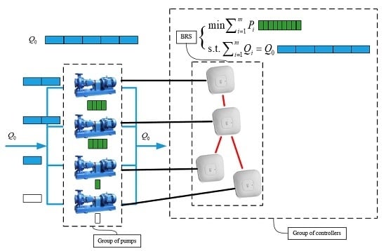
By investigating the existing papers, we summarize them into four groups including rule based methods, mathematical programming, heuristic methods and distributed methods, as shown in

Table 1. Optimization methods for the system with parallel-connected pumps.

Control Framework	Groups	Methods
	Rule based	Zhao et al. [8]; Ma et al. [9]; Gao et al. [10]
Centralized	Mathematical programming	Bonvin et al. [11]; Horváth et al. [12]; Koor et al. [13]
	Heuristic	Wang et al. [17]; Rong et al. [18]; Olszewski et al. [22]
Distributed	Distributed	Dai et al. [24]

. The first three groups are based on the centralized control framework, which replace the group of controllers, as shown in Figure 1, with a single controller. The last group is based on the distributed control framework, as presented in Figure 1.

1.1. Rule Based Methods

In the pump system, the operation still depends on human operators to manage pumps. To tackle this problem, some methods have been conducted on the adjusting pump working, including on-line adaptive control [6] and group control strategy [7]. Zhao et al. [8] defined the most unfavorable thermodynamic loop and used the variable differential pressure set point control strategy of pumps. The test results saved 47–58% water pump power consumption. Ma et al. [9] developed the pressure drop models for water networks and formulated an optimal pump sequence control strategy. The number of pumps in operation was set according to their power consumption and maintenance costs. In addition, Gao et al. [10] proposed a fault-tolerant and energy efficient sequence control strategy (SC) for chilled water pump systems with a differential pressure set-point. The strategy ensured that the water flow of the secondary loop met the primary loop. There was a series of operational problems for the terminal air-handling units and chillers due to the ungratified flow rate demand. Rule based methods are simple and show great performance to meet the demand. The accurate model of pumps is not needed in [8,10]. These methods are widely used in practical engineering. Sometimes pumps cannot work in the most energy efficient way because of the non-optimal working point.

1.2. Mathematical Programming Methods

Currently, many experts have made great efforts on developing and applying methods for pumps working in parallel to improve their energy efficiencies. Many typical research papers were reported by focusing on mathematical programming methods. Bonvin et al. [11] introduced a convex mathematical program for pump scheduling in water networks. It realized an average 3.0% optimality gap and significant saving according to operation costs and energy consumption. Horváth et al. [12] proposed a convex pump model based on pump curves and developed a mixed-integer optimization method. The applicability and results showed that the method was more energy efficient compared with current methods. The errors of the solution and the computation time were influenced by the help variables. In order to keep pumps running close to the best efficiency point, Koor et al. [13] applied the customized optimization software, which adopted the Levenberg–Marquardt algorithm to solve the complex optimization task. By analyzing three different theoretical scenarios, the optimal number of working pumps was estimated. The author in [14] studied the problem of energy consumption minimization for variable speed drive pumps and proposed a simplified convex relaxation of pump characteristics. Two small benchmark networks showed that the method was suitable for pump operations with lower energy costs. To develop an energy-oriented optimal control solution, Jepsen et al. [15] recommended a method to minimize the energy consumption of pump stations by two steps: First, the energy consumption for a pre-selected set of active pumps were formulated as a convex optimization problem, then the problem of choosing the number of active pumps was solved by a convex solver. The proposed solution presumed the performance curves remaining constant over time. Inspired by [15], we adopt the sequential least squares programming algorithm (SLSQP) to compare with our method. The sequential least squares programming algorithm has better computing efficiency [16]. These mentioned mathematical programming algorithms increase the ability to obtain the near-optimal solutions. Due to the equality constraints, there are some deviations to meet the demand. These methods are suitable only for specific systems and lack flexibility.

1.3. Heuristic Methods

Considering the complexity of the problem, some researchers have turned their attention to heuristic optimization methods. By adopting the genetic algorithm, Wang et al. [17] proposed a bi-objective pump scheduling approach. Rong et al. [18] presented a crowding genetic algorithm to decide optimal pump configuration. Cimorelli et al. [19] studied the optimal regulation of pump systems by the genetic algorithm. In addition, Barán et al. [20] introduced a multi-objective evolutionary algorithm to solve the optimal pump scheduling problem with four objectives. Hashemi et al. [21] introduced an ant-colony optimization method to improve the optimization process and reduced the feasible solutions in the search space. The optimization process was repeated many times leading to different costs and the lowest cost was selected. In order to enhance energy conservation and analyze control strategies, Olszewski et al. [22] studied three different strategies for complex pumping stations with a genetic algorithm (GA) and pointed out that minimizing power consumption was the most energy efficient. The ungratified flow rate was affected by the population size. The heuristic optimization methods are powerful tools to solve the optimization problem without any derivatives and continuities assumption. The above methods adopt the advantage of population sampling to solve these combination problems. However, these methods lack convergence guarantee and cannot be used to assess the minimum energy. Under equality constraints, these methods are hard to find a feasible solution. If the system with parallel-connected pumps changes, they need to do the algorithm again.

1.4. Distributed Methods

Recently, we proposed a new building control architecture Insect Intelligent Building ($I^{2}B$) [25]. This new distributed control framework is convenient for pump units. It is open, flexible and has a low configuration cost. There are some early attempts to carry out the distributed control in HVAC systems. Liu et al. [26] developed a decentralized optimization algorithm for optimal set point control for HVAC systems. Dai et al. [24] introduced a novel decentralized transfer algorithm (TA) as a solution to a typical control problem for parallel-connected pumps in HVAC systems. In fact, the idea of distributed control or optimization has been applied widely in other large engineering systems such as the distributed multi-area economic dispatch for active distribution networks [27], or multi-agent traffic light control systems [28].

The above literature review shows that there is great potential in reducing pump energy consumption. Advanced control strategies are effective ways to achieve high energy efficiency. There are three types of methods based on centralized control structures: rule based methods, mathematical programming and heuristic methods. There have also been some distributed methods in recent years that show better flexibility. Dai et al.’s work [24] is an initial attempt to solve the optimization problem for parallel-connected pumps in a distributed manner. We observe that existing studies can be further improved. First, there are some violations of demand constraints. So, strictly speaking, the solutions are not feasible. Second, existing algorithms have no guarantee of convergence. The solution may not be optimal and extra energy is consumed.

In this paper, we consider a distributed pump system, as presented in Figure 1, and extend our previous work [29]. Compared with our previous work, the main differences can be summarized as follows: First, our work considers the controllers connected in the more general topologies and not limited in the chain topology. Second, our work establishes the theoretical convergence results. Motivated by the distributed and peer-to-peer algorithm framework proposed in [25], we put forward a novel distributed optimization method that is suitable for general topologies and establishes theoretical convergence results. Our method consists of two parts: First, in order to process the network information, we apply the breadth first search algorithm to construct a tree to exchange messages. Second, all nodes coordinate with each other and randomly sample a population of speed ratios. In addition, we prove that our method has the guarantee of convergence. Based on a numerical example of pump systems, we compare our approach with other methods. It turns out that our method is able to exactly satisfy the actual demand, minimize energy consumption and has good flexibility. The hardware testing shows that our method can perform on low-cost Raspberry Pi3 and reduce the cost when applied in practical systems.

The remaining part of the paper is organized as follows. In Section 2, we define the speed ratio optimization problem for parallel pumps. In Section 3, we present a novel distributed algorithm for the problem. In Section 4, we prove the convergence of the proposed algorithm. To demonstrate the advantages of the new algorithm, in Section 5, we show numerical results of the algorithm and compare it with the state of art algorithms. We also study the flexibility of the algorithm and test the algorithm on a hardware platform. In Section 6, we conclude the paper.

2. Problem Formulation

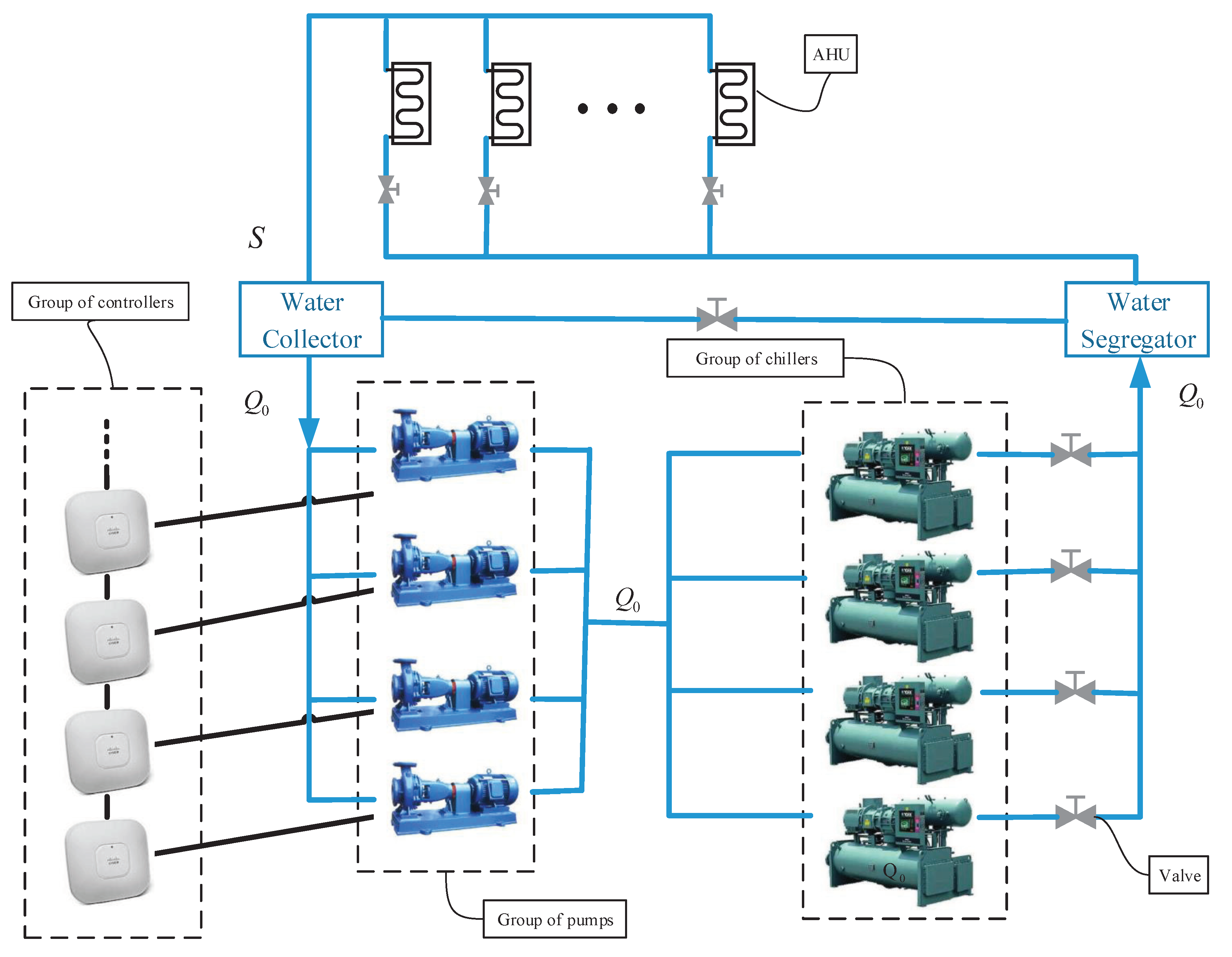
Consider the control of parallel-connected pumps in an HAVC system, as shown in Figure 1. We assume that there are m centrifugal variable-speed pumps connected in parallel and the size of pumps may be different. The demand is a stable value during a period of time (for example, one hour, as given in paper [9]). Our problem is to optimize the number of running pumps and their speed set-points to meet the demand with minimum energy consumption. We also assume that underlying controllers, such as those given in [2], can regulate pump speed to the new set-points in real time.

2.1. Pump Models

Let us first formulate the relationship between pump speed and pump energy consumption. There are various methods to establish the pump model in application, such as dynamic pump model [30], pump approximation model [22]. In order to obtain better precision and convenient calculation, we choose polynomial functions to reflect pump characteristics. It is vital to know pump characteristics to implement optimal pump control. To describe a pump, we need to consider relationships between pump head, flow rate, and efficiency. When pumps work at their rated speeds, the relationships can be indicated by the equations as below.

$$H_i=a_{P1,i}{Q}_i^2+a_{P2,i}{Q}_i+a_{P3,i}$$

(1)

$${\eta }_i=b_{P1,i}{Q}_i^2+b_{P2,i}{Q}_i+b_{P3,i}$$

(2)

$$P_i={\displaystyle \frac{\rho g{Q}_i{H}_i}{1000{\eta }_i{\eta }_{M,i}{\eta }_{VFD,i}}}$$

(3)

We use $H_i$ to denote the head of pump $i,i=1,2,\cdots ,m$ where m is the total number of pumps. $Q_i$ is the flow rate of pump i. ${\eta }_i$ is the mechanical efficiency, $P_i$ is the power consumption of pump i. $P_i$ depends on three sub-efficiency variables, including the mechanical efficiency ${\eta }_i$, the motor efficiency ${\eta }_{M,i}$, the variable frequency efficiency ${\eta }_{VFD,i}$. The $a_{P1,i},a_{P2,i},a_{P3,i},b_{P1,i},b_{P2,i},b_{P3,i}$ are pump performance parameters. These parameters in the equations may be accessed by the pump performance curves or actual measurement data. The data is measured when pumps work at the rated speed. If we obtain the data, it is possible to utilize the least square method to fit the polynomial functions.

We use $n_i$ to denote the actual speed of pump i. $n_{0,i}$ is the rated speed of pump i. We define speed ratio ${\omega }_i$ to depict the ratio between the actual speed and the rated speed.

$${\omega }_i=\frac{n_i}{n_{0,i}}$$

(4)

In general, the pump performance parameters are related to the speed and the operating conditions. When pump works in variable speed status and the operating conditions do not change, we can attain a series of pump characteristic curves through the pump affinity laws [31], as presented in Equation (5).

$$\begin{array}{cc}\hfill & Q_i\left(n_{0,i}\right)=\frac{Q_i\left(n_i\right)}{{\omega }_i}\hfill \\ \hfill & H_i\left(n_{0,i}\right)=\frac{H_i\left(n_i\right)}{{\omega }_i^2}\hfill \\ \hfill & {\eta }_i\left(n_{0,i}\right)={\eta }_i\left(n_i\right)\hfill \end{array}$$

(5)

where $Q_i\left(n_{0,i}\right)$ is the rated flow rate at rated speed $n_0$, $Q_i\left(n_i\right)$ is the actual flow rate at actual speed $n_i$. $H_i\left(n_{0,i}\right)$ is the rated head at rated speed $n_0$. $H_i\left(n_i\right)$ is the actual head at actual speed $n_i$. ${\eta }_i\left(n_{0,i}\right)$ is the rated mechanical efficiency at rated speed $n_0$. Using the pump affinity laws and Equations (1) and (2), we can reach the equations of pump head and flow rate, efficiency and flow rate at a speed $n_i$ including rated and non-rated, which are as below.

$$H_i=a_{P1,i}{Q_i}^2+a_{P2,i}{\omega }_i{Q}_i+a_{P3,i}{{\omega }_i}^2$$

(6)

$${\eta }_i=b_{P1,i}{\left(\frac{Q_i}{{\omega }_i}\right)}^2+b_{P2,i}\left(\frac{Q_i}{{\omega }_i}\right)+b_{P3,i}$$

(7)

Although paper [32] indicated that ${\eta }_{M,i},{\eta }_{VFD,i}$ depended on ${\omega }_i$, when the speed ratios meet $0.4\le {\omega }_i\le 1$, ${\eta }_{M,i},{\eta }_{VFD,i}$ could supposedly be constants. The reason is that ${\omega }_i$ has little influence on them. Therefore, we can dispense with the impact of ${\eta }_{M,i},{\eta }_{VFD,i}$ and only consider the mechanical efficiency ${\eta }_i$. As a result, the pump power consumption equation can be rewritten as below.

$$P_i={\displaystyle \frac{\rho g{Q}_i{H}_i}{1000{\eta }_i}}$$

(8)

When the demand is given, in Figure 1 the total demand pressure set point $H_0$ and the total demand flow rate $Q_0$ meet the resistance characteristic equation of the pipe net as follows [33]:

$$H_0=S{Q}_0^2$$

(9)

where S is the resistance of the pipe net. This equation makes sure that if the total flow rate on the main pipe is $Q_0$ and S does not change, it can keep the total pressure equal to the demand pressure set point $H_0$. Once S changes, it leads to a different demand.

2.2. Optimization Problem Formulation

Now let us formulate the pump speed ratio optimization problem (PSROP).

Problem 1.

Pump Speed Ratio Optimization Problem (PSROP).

$$\underset{{\omega }_i,i\in \{1,2,...m\}}{min}\sum _{i=1}^m{P}_i\left({\omega }_i\right)$$

(10)

$$s.t.H_0=H_i$$

(11)

$$Q_0=\sum _{i=1}^m{Q}_i$$

(12)

$${\omega }^{-}\le {\omega }_i\le 1or{\omega }_i=0,i\in \{1,2,...,m\}$$

(13)

The objective function presents that the optimization objective of this paper is to minimize the total power consumption of pumps in parallel. The objective function indicates that we should try to find a combination of ${\omega }_i$ to content the corresponding constraints at the lowest energy consumption. Constraint (11) is the equality relationship between the head of the pump and the demand total pressure $H_0$. Constraint (12) is to guarantee that the amount of flow rate is equal to the total demand flow rate $Q_0$ on the main pipe. Constraint (13) is the range of the speed ratio. ${\omega }^{-}$ is the lower limitation of the speed ratio. If the speed ratio is equal to 0, it means that the pump i is shut down.

3. Proposed Algorithm

In this section, we propose a novel algorithm, breadth first search random sampling (BRS for short), to solve the optimization problem PSROPred (Pump Speed Ratio Optimization Problem). Our algorithm includes two steps.

First, in order to process the network information, we apply the breadth first search algorithm (BFS) [34] to construct a spanning tree supporting the communication in the pump intelligent node network. For details of the BFS algorithm, see Appendix A.1 in Appendix A.

Second, based on the tree, we randomly sample the speed ratios. All the nodes coordinate with each other, carry out parallel calculations to optimize the speed ratio of each node so that the total energy consumption is minimized. Before introducing the algorithm in detail, we make an assumption as follows:

Assumption 1.

In our distributed pump control system, every pump is an intelligent node equipped with a controller. The pump model and an identical computing program have been stored in the node (controller) for the pump. The node can communicate with neighbors and do calculations. The network of the pump intelligent nodes forms a connected graph.

With this assumption, if node i and node j are not neighbors, there is at least one path between them.

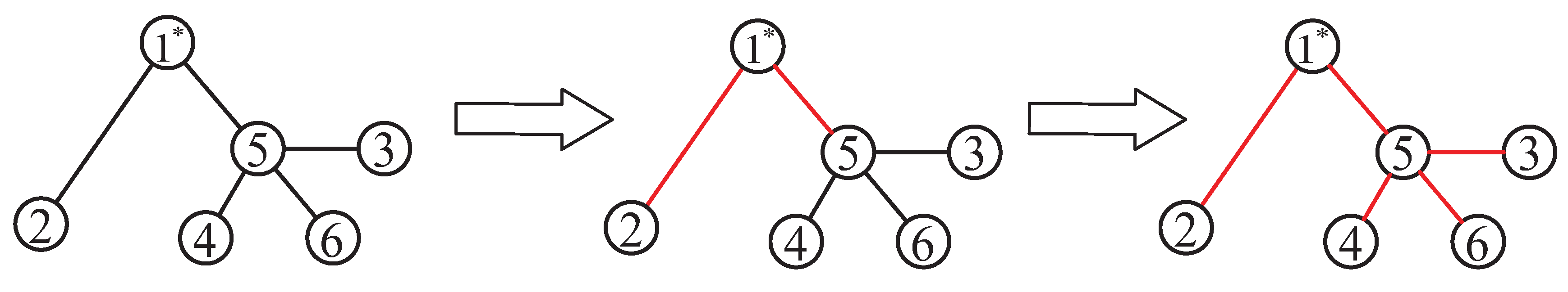
Figure 2 gives an example of constructing a BFS tree for a network with six nodes (controllers for six pumps connected in parallel). From the root node 1, the search message indicated by red links gradually spreads to leaf nodes. Based on the BFS tree, every node performs an algorithm enabling coordinations with its neighbors.

Our algorithm is formally defined as Algorithm 1. Algorithm 1 uses the BFS tree generated by the BFS algorithm defined in Appendix A.1 in Appendix A as input and calls the Algorithm defined in Appendix A.2 in Appendix A to do the message processing. A message processing example is shown in Figure 3 based on the BFS tree given in Figure 2. The messaging mechanism between nodes can be described as follows. Every node has six input message queues. Each message queue records the message. Once the message is read, it will be deleted from the queue. The communication between nodes is synchronous. During the k-th round, each node sends messages to its neighbors and reads from its input message queues. As a result, the messages of all child nodes are collected.

Below is a description of the main procedure in Algorithm 1. Every node obtains its node type in the BFS tree (as root node, intermediate node, or leaf node). Then every node initializes its pump performance parameters, the range of speed ratio, the sample adjustment parameter $\tau$, the child nodes set ${\mathcal{N}}_i$ and the total iteration parameter K.

Every leaf node independently generates speed ratio samples following the uniform distribution over the interval $[{\omega }^{-}-\tau ,1]$ with ${\omega }_{i,k}$ as the k-th sample of node i. If the speed ratio sample ${\omega }_{i,k}\ge {\omega }^{-}$, it will evaluate corresponding $Q_{i,k},P_{i,k}$. If not, the node will set the sample to 0, which means the pump will be shut down. Then the node will transmit the $Q_{T,i,k},P_{T,i,k},{\omega }_{T,i,k}$ to its parent node. If it does not receive end instruction, the leaf node will continue to do the above operation. When the leaf node receives end instruction from the parent, it will stop generating samples, and acquire its optimal speed ratio. The intermediate node performs the same operation that generates samples. The difference is that the intermediate node will calculate the partial summation flow rate $Q_{T,i,k}$ and the partial summation power consumption $P_{T,i,k}$ over the subtree of node i basing on the $Q_{T,j,k_j}$, $P_{T,j,k_j}$ provided by its child nodes ${\mathcal{N}}_i$. The $Q_{T,j,k_j}$, $P_{T,j,k_j}$ is read from the input message queue. Next, if the partial summation flow rate $Q_{T,i,k}\le Q_0$, the intermediate node will transmit $Q_{T,i,k},P_{T,i,k},{\omega }_{T,i,k}$ to its parent node. If not, the node will delete the $Q_{T,i,k},P_{T,i,k},{\omega }_{T,i,k}$. As for the root node, it will compute its $Q_{i,k}$ through the total flow rate $Q_0$ and the $Q_{T,j,k_j}$ provided by its child nodes. This operation makes sure that the constraint is satisfied. In view of the $Q_i$, the root node utilizes the Equations (6)–(8) and $H_0$ to compute ${\omega }_{i,k}$. When ${\omega }_{i,k}$ satisfies the speed ratio range constraint, it will calculate the total energy consumption $P_{T,i,k}$. $P_k^{\ast }$ is the currently optimal total energy consumption after k rounds selection of speed ratio samples. ${\tilde{\omega }}_k^{\ast }$ denotes the optimal estimation combination of speed ratio samples in the k-th round for the root node. In addition, if $P_{T,i,k}\le P_k^{\ast }$, the root node will update $P_k^{\ast }$ and ${\tilde{\omega }}_k^{\ast }$ to save the currently optimal estimation combination of speed ratios for the whole network. By doing so, after K rounds the root node supposes that the best combination of speed ratios is achieved, and therefore ends the entire algorithm and sends the best combination of speed ratios ${\tilde{\omega }}_k^{\ast }$ to child nodes. Once the node receives the end message and ${\tilde{\omega }}_k^{\ast }$, it will stop calculation and send them to child nodes.

From the steps of Algorithm 1, we can observe that the BRS algorithm makes sure the solution exactly meets the demand (the total flow rate constraint). Every node maintains its own speed ratio ${\tilde{\omega }}_i^{\ast }$. The whole adjustment is an iterative optimization process with the cooperation of each node. Constraints are satisfied in the entire iteration process. Furthermore, it has the flexibility due to the distributed control structure. We will prove that the total energy consumption can be minimized.

Algorithm 1: Breadth first search random sampling algorithm (BRS)

4. Theoretical Analysis of the Proposed Algorithm

We carry out a theoretical analysis of the convergence for the proposed BRS algorithm. According to the definition of the algorithm, the sample process at node i (for pump i ) of speed ratio can be viewed as an i.i.d. stochastic process $\{{\omega }_{i,k},k=1,2,...\}$ where ${\omega }_{i,k}$ is the k-th sample of the speed ratio of pump i. The speed ratio sample of pump i follows the uniform distribution

$$U[{\omega }^{-}-\tau ,1]$$

(14)

with $\tau >0$ as a given parameter such that ${\omega }^{-}>\tau$.

Assumption 2.

Both the energy consumption function $P_i\left({\omega }_i\right)$ and flow rate function $Q_i\left({\omega }_i\right)$ of a pump are continuous functions on the domain $\left\{0\right\}\cup [{\omega }^{-}-\tau ,1]$ with $P_i\left(0\right)=Q_i\left(0\right)=0$. The flow rate function $Q_i\left({\omega }_i\right)$ of a pump is also a monotonously increasing function.

Now we are ready to show the main theoretical result: the speed ratios of the m pumps output by our BRS algorithm will converge to the optimal solution of the PSROP problem (defined in Section 2.2 by Equations (10)–(13) if K goes to infinity. According to the steps of the BRS algorithm, under Assumption 1, all pump nodes are divided into three types on the spanning tree T. Denote $\mathcal{I}$ as the set of intermediate nodes, $\mathcal{L}$ as the set of leaf nodes, $\mathcal{R}=\left\{r\right\}$ as the set of a single root node. Then we can rewrite PSROP in an equivalent form.

Problem 2.

Alternative Pump Speed Ratio Optimization Problem (PSROP’)

$$\underset{{\omega }_i,i\in \mathcal{L}\cup \mathcal{I}\cup \left\{r\right\}}{min}\sum _{i\in \mathcal{L}\cup \mathcal{I}\cup \left\{r\right\}}{P}_i\left({\omega }_i\right)$$

(15)

$$s.t.H_0=H_{i}i\in \mathcal{L}\cup \mathcal{I}\cup \left\{r\right\}$$

(16)

$$Q_0=\sum _{i\in \mathcal{L}\cup \mathcal{I}\cup \left\{r\right\}}{Q}_i$$

(17)

$${\omega }^{-}\le {\omega }_i\le 1or{\omega }_i=0,i\in \mathcal{L}\cup \mathcal{I}\cup \left\{r\right\}$$

(18)

It is trivial that the optimal value of PSROP’ is the same as that of PSROP since both objective functions and constraints are the same when we re-order the speed ratios. Below, in order to present our analysis, we define the optimal pump speed ratios according to node types of the spanning tree T as follows

$${\omega }_T^{\ast }=[{\omega }_i^{\ast },i\in \mathcal{L}\cup \mathcal{I}\cup \left\{r\right\}]$$

(19)

Similarly, we denote

$${\omega }_T=[{\omega }_i,i\in \mathcal{L}\cup \mathcal{I}\cup \left\{r\right\}]$$

(20)

as the combination list of decision variables for the PSROP’ problem and

$${\tilde{\omega }}_{T,K}^{\ast }=[{\tilde{\omega }}_{i,K}^{\ast },i\in \mathcal{L}\cup \mathcal{I}\cup \left\{r\right\}]$$

(21)

as the speed ratios of the m pumps output by our BRS algorithm after K rounds to emphasis the role of node type on the tree T. We note that due to the equality constraint Equation (17), the optimal speed ratio ${\omega }_r^{\ast }$ of the root node r can be written as a function of speed ratios of other nodes. In fact, we have (due to the monotone property of flow rate function by Assumption 2)

$${\omega }_r^{\ast }=Q_r^{-1}(Q_0-\sum _{i\in \mathcal{L}\cup \mathcal{I}}{Q}_i\left({\omega }_i^{\ast }\right))$$

(22)

Similarly, we have

$${\tilde{\omega }}_{r,K}^{\ast }=Q_r^{-1}(Q_0-\sum _{i\in \mathcal{L}\cup \mathcal{I}}{Q}_i\left({\tilde{\omega }}_{i,K}^{\ast }\right))$$

(23)

according to the step in Line 20 of Algorithm 1 running at the root node.

Assumption 3.

${\omega }_r^{\ast }\in ({\omega }^{-},1)$ and ${\sum }_{i\in \mathcal{L}\cup \mathcal{I}}{Q}_i\left({\omega }_i^{\ast }\right)>0$.

Theorem 1.

Suppose Assumptions 1, 2, 3 are satisfied. Let $\epsilon >0$ be any given positive number, then

$$\underset{K\to \infty }{lim}Pr\left\{\right|P\left({\tilde{\omega }}_{T,K}^{\ast }\right)-P\left({\omega }_T^{\ast }\right)|<\epsilon \}=1$$

(24)

where ${\tilde{\omega }}_{T,K}^{\ast }=[{\tilde{\omega }}_{i,K}^{\ast },i\in \mathcal{L}\cup \mathcal{I}\cup \left\{r\right\}]$ are speed ratios output by the algorithm after K rounds.

Proof of Theorem 1.

From Assumption 3, we know that ${\omega }_r^{\ast }\in ({\omega }^{-},1)$ and ${\sum }_{i\in \mathcal{L}\cup \mathcal{I}}{Q}_i\left({\omega }_i^{\ast }\right)>0$. In this case, we know that $Q_r\left({\omega }_r^{\ast }\right)>0$ and $\exists i_0\in \mathcal{L}\cup \mathcal{I}$ such that

$$Q_{i_0}\left({\omega }_i^{\ast }\right)>0$$

(25)

We must have $Q_r\left({\omega }_r^{\ast }\right)\in [Q_r\left({\omega }^{-}\right),Q_0)$ and $Q_{i_0}\left({\omega }_{i_0}^{\ast }\right)\in (0,Q_0)$

Since both $Q_r$ and $P_r$ are continuous (by Assumption 2), for any ${\epsilon }_1>0$, there exists a ${\delta }_r\left({\epsilon }_1\right)\in (0,1-{\omega }^{-})$ such that $\forall {\omega }_r\in [{\omega }_r^{-}\left({\epsilon }_1\right),{\omega }_r^{\ast }]$, where ${\omega }_r^{-}\left({\epsilon }_1\right)={\omega }_r^{\ast }-{\delta }_r\left({\epsilon }_1\right)$. It is true that

$$Q_r\left({\omega }_r\right)\in (Q_r\left({\omega }_r^{\ast }\right)-{\epsilon }_1,Q_r\left({\omega }_r^{\ast }\right)]$$

(26)

$$P_r\left({\omega }_r\right)\in (P_r\left({\omega }_r^{\ast }\right)-{\epsilon }_1,P_r\left({\omega }_r^{\ast }\right)+{\epsilon }_1)$$

(27)

Similarly, since both $Q_i$ and $P_i$ are continuous (by Assumption 2), when $Q_i\left({\omega }_i^{\ast }\right)>0$ (then ${\omega }_i^{\ast }\in [{\omega }^{-},1]$), for any ${\epsilon }_2>0$, there exists a ${\delta }_i\left({\epsilon }_2\right)\in (0,1-{\omega }^{-})$ such that $\forall {\omega }_i\in {\mathit{B}}_{\mathbf{i}}=[{\omega }_i^{\ast },{\omega }_i^{+}\left({\epsilon }_2\right)]$,

$${\mathit{B}}_{\mathit{i}}=[{\omega }_i^{\ast },{\omega }_i^{+}\left({\epsilon }_2\right)]$$

(28)

and ${\omega }_i^{+}\left({\epsilon }_2\right)={\omega }_i^{\ast }+{\delta }_i\left({\epsilon }_2\right)$, it is true that

$$Q_{}\left({\omega }_i\right)\in [Q_i\left({\omega }_i^{\ast }\right),Q_i\left({\omega }_i^{\ast }\right)+{\epsilon }_2)$$

(29)

$$P_i\left({\omega }_i\right)\in (P_i\left({\omega }_i^{\ast }\right)-{\epsilon }_2,P_i\left({\omega }_i^{\ast }\right)+{\epsilon }_2)$$

(30)

When ${\omega }_i^{\ast }=0$, then $Q_i\left({\omega }_i^{\ast }\right)=0$, we set ${\mathit{B}}_i=\left\{0\right\}$. For this case, $\forall {\omega }_i\in {\mathit{B}}_i$, Equations (29) and (30) still hold.

Since the optimal solution is feasible, we have

$$Q_0=Q_r\left({\omega }_r^{\ast }\right)+\sum _{i\in \mathcal{L}\cup \mathcal{I}}{Q}_i\left({\omega }_i^{\ast }\right)$$

(31)

For a given ${\epsilon }_1>0$ and corresponding ${\delta }_r\left({\epsilon }_1\right)$, we choose ${\epsilon }_2$ in Equations (29) and (30) such that

$$(m-1){\epsilon }_2\le Q_r\left({\omega }_r^{\ast }\right)-Q_r\left({\omega }_r^{-}\left({\epsilon }_1\right)\right)$$

(32)

or equivalently

$$\sum _{i\in \mathcal{L}\cup \mathcal{I}}{Q}_i\left({\omega }_i^{\ast }\right)+(m-1){\epsilon }_2\le Q_0-Q_r\left({\omega }_r^{-}\left({\epsilon }_1\right)\right)$$

(33)

For $({\omega }_i,i\in \mathcal{L}\cup \mathcal{I})$ satisfying ${\cap }_{i\in \mathcal{L}\cup \mathcal{I}}{B}_i$, we have

$${\omega }_r=Q_r^{-1}(Q_0-\sum _{i\in \mathcal{L}\cup \mathcal{I}}{Q}_i\left({\omega }_i\right))$$

(34)

$${\omega }_r=Q_r^{-1}(Q_r\left({\omega }_r^{\ast }\right)+\sum _{i\in \mathcal{L}\cup \mathcal{I}}(Q_i\left({\omega }_i^{\ast }\right)-Q_i\left({\omega }_i\right)))\ge Q_r^{-1}(Q_r\left({\omega }_r^{\ast }\right)-(m-1){\epsilon }_2)$$

(35)

$${\omega }_r\ge Q_r^{-1}\left(Q_r\left({\omega }_r^{-}\left({\epsilon }_1\right)\right)\right)={\omega }_r^{-}\left({\epsilon }_1\right)$$

(36)

From the monotone property of $Q_r^{-1}$ (based on the monotone property of flow rate function by Assumption 2), we also have

$${\omega }_r\le Q_r^{-1}\left(Q_r\left({\omega }_r^{\ast }\right)\right)={\omega }_r^{\ast }$$

(37)

So

$${\omega }_r\in [{\omega }_r^{-}\left({\epsilon }_1\right),{\omega }_r^{\ast }]$$

(38)

From Equation (30) and $P_i\left({\omega }_i\right)$ is set to 0 if ${\omega }_i=0$, we know that

$$\sum _{i\in \mathcal{L}\cup \mathcal{I}}|P_i\left({\omega }_i\right)-P_i\left({\omega }_i^{\ast }\right)|<(m-1){\epsilon }_2$$

(39)

Due to Equation (28), for ${\omega }_r$ in Equation (34) we have

$$P_r\left({\omega }_r\right)\in (P_r\left({\omega }_r^{\ast }\right)-{\epsilon }_1,P_r\left({\omega }_r^{\ast }\right)+{\epsilon }_1)$$

(40)

In sum, we have

$$|\sum _{i\in \mathcal{L}\cup \mathcal{I}\cup \left\{r\right\}}{P}_i\left({\omega }_i\right)-P\left({\omega }^{\ast }\right)|=|\sum _{i\in \mathcal{L}\cup \mathcal{I}\cup \left\{r\right\}}(P_i\left({\omega }_i\right)-P\left({\omega }_i^{\ast }\right))|<Q_r\left({\omega }_r^{\ast }\right)-Q_r\left({\omega }_r^{-}\left({\epsilon }_1\right)\right)+{\epsilon }_1$$

(41)

For given $\epsilon >0$, we can choose ${\epsilon }_1$ such that

$$Q_r\left({\omega }_r^{\ast }\right)-Q_r\left({\omega }_r^{-}\left({\epsilon }_1\right)\right)+{\epsilon }_1<\epsilon$$

(42)

For nodes $i\in \mathcal{L}\cup \mathcal{I}$, define ${\mathit{A}}_{i,k}$ as the event that the kth sample ${\omega }_{i,k}$ generated at node i belongs to the interval ${\mathit{B}}_i$ defined in Equation (28) with the understanding that ${\mathit{B}}_i=\left\{0\right\}$ if ${\omega }_{i,k}=0$ (corresponding to the case $u_{i,k}\in [{\omega }^{-}-\tau ,{\omega }^{-})$. According to the algorithm design, we have

$$Pr\left\{{\mathit{A}}_{i,k}\right\}=Pr\{{\omega }_{i,k}\in {\mathit{B}}_i\}={\displaystyle \frac{{\omega }_i^{+}-{\omega }_i^{\ast }}{1-({\omega }^{-}-\tau )}}$$

(43)

if $Q_i\left({\omega }_i^{\ast }\right)>0$, or

$$Pr\left\{{\mathit{A}}_{i,k}\right\}=Pr\{{\omega }_{i,k}\in {\mathit{B}}_i\}=Pr\{u_{i,k}\in [{\omega }^{-}-\tau ,{\omega }^{-})\}={\displaystyle \frac{\tau }{1-({\omega }^{-}-\tau )}}$$

(44)

if $Q_i\left({\omega }_i^{\ast }\right)=0$, it means the pump will be shut down. Since the samples generated at different nodes in $\mathcal{L}\cup \mathcal{I}$ are independent, we have

$$Pr\left\{\bigcap _{i\in \mathcal{L}\cup \mathcal{I}}{\mathit{A}}_{i,k}\right\}=\prod _{i\in \mathcal{L}\cup \mathcal{I}}Pr\left\{{\mathit{A}}_{i,k}\right\}\ge {\left[{\displaystyle \frac{d}{1-({\omega }^{-}-\tau )}}\right]}^{m-1}$$

(45)

where d is a constant no larger than $\tau$ and $({\omega }_i^{+}-{\omega }_i^{\ast })$ for nodes $i\in \mathcal{L}\cup \mathcal{I}$ such that $Q_i\left({\omega }_i^{\ast }\right)>0$.

From Equation (33), we know that if ${\omega }_{i,k}\in {\mathit{B}}_i$, $\forall i\in \mathcal{L}\cup \mathcal{I}$, it is true that

$$\sum _{i\in \mathcal{L}\cup \mathcal{I}}{Q}_i\left({\omega }_{i,k}\right)<Q_0$$

(46)

As a result, ${\omega }_{T,k}=[{\omega }_{i,k},i\in \mathcal{L}\cup \mathcal{I};{\omega }_{r,k}]$ where

$${\omega }_{r,k}=Q_r^{-1}(Q_0-\sum _{i\in \mathcal{L}\cup \mathcal{I}}{Q}_i\left({\omega }_{i,k}\right))$$

(47)

forms a feasible solution with total energy consumption as

$$P\left({\omega }_{T,k}\right)=\sum _{i\in \mathcal{L}\cup \mathcal{I}\cup r}{P}_i\left({\omega }_{i,k}\right)$$

(48)

From the selection of ${\tilde{\omega }}_{T,k}^{\ast }$ as the feasible solution with the lowest total energy consumption for the first k-th rounds, we have

$$P\left({\tilde{\omega }}_{T,k}^{\ast }\right)\le P\left({\omega }_{T,k}\right)$$

(49)

From the optimality of ${\omega }^{\ast }$ and Equation (41), we have

$$P\left({\omega }^{\ast }\right)\le P\left({\tilde{\omega }}_{T,k}^{\ast }\right)\le P\left({\omega }_{T,k}\right)\le P\left({\omega }^{\ast }\right)+\epsilon$$

(50)

The theorem is proved. □

As a result, the BRS algorithm can not only exactly meet the constraints and have great flexibility but also has the guarantee of convergence. By applying the BRS algorithm, the solution ${\tilde{\omega }}_{T,k}^{\ast }$ converges to the optimal speed ratio ${\omega }^{\ast }$ in probability. Hence, under Assumption 1, BRS algorithm is easy to realize and can converge to the optimal solution.

Remark 1.

In reality, we cannot judge whether Assumption 3 holds in advance. To make sure of the convergence to the global true optimal solution, we can run the algorithm with each node as the root node in turn and compare the final results.

5. Results and Discussion

In this section, we will verify the properties of the proposed BRS algorithm including the demand satisfaction, minimum energy consumption, the flexibility in adapting to changing the topology of pump systems and the low-cost hardware test. We compare BRS with other methods in demand satisfaction and energy consumption. This section is organized as follows: First, we introduce the study cases, the simulation environment and compared algorithms. Second, we study the violation of constraint satisfaction among BRS and the compared algorithms. Third, we compare the performance among BRS and other algorithms. Then, we study the flexibility of BRS under a different number of intelligent nodes. Finally, we test BRS based on low-cost hardware.

5.1. Set up of Study Cases

We adopt the performance parameters of pumps that are introduced in paper [35].

Table 2. Performance parameters of pumps.

Pump	Performance Parameters
	${\mathit{a}}_{\mathit{P}\mathbf{1}\mathit{,}\mathit{i}}$	${\mathit{a}}_{\mathit{P}\mathbf{2}\mathit{,}\mathit{i}}$	${\mathit{a}}_{\mathit{P}\mathbf{3}\mathit{,}\mathit{i}}$	${\mathit{b}}_{\mathit{P}\mathbf{1}\mathit{,}\mathit{i}}$	${\mathit{b}}_{\mathit{P}\mathbf{2}\mathit{,}\mathit{i}}$	${\mathit{b}}_{\mathit{P}\mathbf{3}\mathit{,}\mathit{i}}$
PUMP-A	−0.0046	0.0696	60.271	−0.0002	0.0254	0.0616
PUMP-B	−0.0112	0.1358	54.841	−0.0005	0.0316	0.2582

shows the specific parameters and performance curves of the pumps that are presented in Figure 4. The parameters are collected from the RXL (Hot cold water vertical) type pumps.

Here, we establish an HVAC system including six pumps in parallel. Four of the pumps are PUMP-A (big pump) and two of the pumps are PUMP-B (small pump). The pump with a relatively higher capacity of flow rate is named big pump and the other one is small pump [35]. We adopt four different total flow rate and head demand cases in an HVAC system, which represent the typical stable working conditions during a period of time, as shown in

Table 3. Different demands of the heating, ventilation, and air-conditioning (HVAC) system.

	${\mathit{H}}_0$(m)	${\mathit{Q}}_0$(L/s)
Case 1	26	86
Case 2	29	117
Case 3	36	248
Case 4	39	288

. These cases are from light to heavy. In order to investigate a method in depth, the optimal working positions for parallel pumps are different under these four cases.

5.2. Software Simulation Environment

The software simulation environment is shown in

Table 4. The simulation environment for different methods.

Algorithm	Control Framework	Simulation Environment
BRS	Distributed	DSP
SC	Centralized	Python
SLSQP	Centralized	Python
GA	Centralized	Python
TA	Distributed	DSP

. The centralized algorithms SC, SLSQP (Sequential least squares programming algorithm) and GA are built with an open-source software Python with version 2.7 to carry out the simulation. We employ the distributed simulation platform (DSP). (DSP is a simulation engine written in Python that can simulate distributed algorithms synchronous to all nodes through UDP (User Datagram Protocol) communication.) To investigate the performance of both BRS and TA. The operating environment is Win10x64, Intel (R) Core (TM) i7-7700 @3.60GHz, DSP1.0, and computer memory is 8 GB. Based on the DSP, we can simulate a distributed pump system to test BRS and TA algorithms under different HVAC system demands. DSP can generate different kinds of topologies. TA is designed under controllers connected in the chain topology and relaxes the constraint. If the topology changes, TA cannot obtain the violation of constraints. All nodes are connected one by one for distributed methods in Section 5.4. In Section 5.6, we adopt a tree topology. The population size and iterations are the same for GA and BRS.

5.3. Other Algorithms to Be Compared with BRS

The compared algorithms include centralized algorithms and distributed algorithms. We pick up three typical centralized algorithms including sequence control strategy (SC) [10], sequential least squares programming algorithm (SLSQP) [16] and genetic algorithm (GA) [22]. The distributed transfer algorithm (TA) was proposed in [24]. These algorithms are selected based on a previous literature review. They are well represented characteristics of the four class methods and show good performance. The details of these algorithms are referred to in the related literature.

5.4. The Violation of Constraint Satisfaction

Table 5. Numerical comparison for different study cases.

Case	Method	PUMP-A		PUMP-A		PUMP-A		PUMP-A		PUMP-B		PUMP-B		$\mathsf{\Delta }$ (L/s)	${\mathit{P}}^{\mathbf{*}}$ (KW)
		${\mathit{\omega }}_{\mathbf{1}}$	${\mathit{Q}}_{\mathbf{1}}$	${\mathit{\omega }}_{\mathbf{2}}$	${\mathit{Q}}_{\mathbf{2}}$	${\mathit{\omega }}_{\mathbf{3}}$	${\mathit{Q}}_{\mathbf{3}}$	${\mathit{\omega }}_{\mathbf{4}}$	${\mathit{Q}}_{\mathbf{4}}$	${\mathit{\omega }}_{\mathbf{5}}$	${\mathit{Q}}_{\mathbf{5}}$	${\mathit{\omega }}_{\mathbf{6}}$	${\mathit{Q}}_{\mathbf{6}}$
Case 1	BRS	0.7340	43.476	0.7304	42.524	0	0	0	0	0	0	0	0	0	25.378
	SC	0.7199	39.623	0	0	0	0	0	0	0.9	46.377	0	0	0	32.970
$Q_0=86$	SLSQP	0.7322	42.995	0.7322	42.995	0	0	0	0	0	0	0	0	−0.01	25.377
	GA	0.8046	59.632	0	0	0	0	0	0	0.7528	26.342	0	0	0.026	26.902
	TA	0.7354	43.831	0	0	0	0	0	0	0.7269	21.296	0.7269	21.296	0.423	27.288
Case 2	BRS	0.8285	58.509	0.8284	58.491	0	0	0	0	0	0	0	0	0	38.757
	SC	0.9066	74.038	0	0	0	0	0	0	0.9	42.962	0	0	0	45.697
$Q_0=117$	SLSQP	0.8285	58.509	0.8285	58.509	0	0	0	0	0	0	0	0	0.018	38.764
	GA	0.7835	48.045	0.8798	68.960	0	0	0	0	0	0	0	0	−0.005	39.539
	TA	0.7790	46.901	0.7803	47.255	0	0	0	0	0.7710	23.201	0	0	0.357	39.614
Case 3	BRS	0.9051	61.208	0.9111	62.552	0.9076	61.775	0.9107	62.465	0	0	0	0	0	101.322
	SC	0.9	60.036	0.9	60.036	0.9046	61.098	0	0	0.9	33.415	0.9	33.415	0	105.609
$Q_0=248$	SLSQP	0.9086	61.991	0.9086	61.991	0.9086	61.991	0.9086	61.991	0	0	0	0	−0.036	101.317
	GA	0.9516	71.161	0.8425	45.289	0.9798	76.739	0.8780	54.792	0	0	0	0	−0.019	103.741
	TA	0.8833	56.087	0.8762	54.349	0.8762	54.349	0.8832	56.076	0.8665	27.381	0	0	0.242	102.540
Case 4	BRS	0.9264	60.082	0.9417	63.626	0.9597	67.610	0.9667	69.121	0.8972	27.561	0	0	0	129.493
	SC	0.9	53.510	0.9	53.510	0.9	53.510	0.9	53.510	1.0	44.156	0.9086	29.804	0	134.518
$Q_0=288$	SLSQP	0.9742	70.722	0.9742	70.722	0.9742	70.722	0.9742	70.722	0.8402	5.106	0	0	−0.006	131.494
	GA	0.9497	65.410	0.8780	47.457	0.9587	67.390	0.9593	67.523	0.9717	40.189	0	0	−0.031	131.937
	TA	0.9193	58.378	0.9193	58.378	0.9193	58.378	0.9120	56.568	0.9018	28.494	0.8973	27.574	−0.23	130.327

presents the calculation results for five algorithms listed in Section 5.3 and for four cases listed in Section 5.1. $\Delta$ represents the violation of constraint (12), which means that $\Delta =\sum Q_i-Q_0$. The total flow rate exceeds the actual demand if $\Delta$ is positive. The total flow rate is less than the actual demand if $\Delta$ is negative. From Table 5, $\Delta$ related to BRS and SC are all 0 in the four cases and there are no violations to meet the constraint. As can be seen, $\Delta$ for the other three algorithms are positive or negative.

The reason for the performance difference among algorithms in constraint satisfaction for pump systems is that their principles are different. Our BRS algorithm and SC deal with the equality constraint directly. The BRS algorithm uses the advantage of population sampling and the equality constraint to find feasible solutions. SC adopts the PID (Proportion Integration Differentiation) feedback control to eliminate the deviation and meet the constraint. The other three methods relax the equality constraint and adopt the penalty function. They cannot meet the constraint. Regardless of cases, $\Delta$ is distributed randomly.

Experimental results prove that most methods have some violations to meet the demand. Furthermore, data comparison of $\Delta$ confirms that our BRS algorithm can exactly satisfy the demand constraints, which is difficult for most methods.

From Table 5, we can also see that when the demand changes, BRS can automatically regulate the number of working pumps and their speed ratios. In addition, we apply BRS to a very light demand $H_0=20,Q_0=20$. The result of our BRS algorithm only opens a PUMP-B and its ${\omega }_{\mathrm{5}}=0.6438,Q_{\mathrm{5}}=20$.

5.5. Performance Comparison

Table 5 summarizes the total energy consumption $P^{\ast }$ for five algorithms listed in Section 5.3 and for four cases listed in Section 5.1. The bold value of $P^{\ast }$ in each cases is the minimum energy consumption. When comparing $P^{\ast }$ of BRS to that of SC in the four cases, it is clear that the energy consumption of BRS is the minimum to exactly meet the demand constraint. Comparing $P^{\ast }$ among BRS and other three algorithms in the four cases, the energy consumption of BRS is the minimum in Case 2 and Case 4. The energy consumption of SLSQP is slightly lower than BRS in Case 1 and Case 3. The reason is that the solutions of SLSQP are not feasible and the total flow rate is less than the actual demand. Due to providing less flow rate, the energy consumption of SLSQP is minimum. The differences of $P^{\ast }$ between SLSQP and BRS are $0.001$ and $0.005$ in Case 1 and Case 3. Table 5 shows that SC can satisfy the demand constraint. However, SC does not optimize the energy consumption and pumps work in the non-optimal points. As a result, SC consumes much more energy.

According to these findings, due to lacking the guarantee of convergence, these methods cannot work optimally in most cases. Our BRS algorithm makes sure to satisfy the demand and minimize the energy consumption of pumps. It consumes less energy in the four cases and verifies the guarantee of convergence.

From Table 5, it can be observed that there are different combinations of pumps for type PUMP-A and type PUMP-B in the four proposed cases. In Case 1, we can choose the first option to open two PUMP-A, the second option to open one PUMP-A and two PUMP-B or the third option to open one PUMP-A and one PUMP-B. BRS algorithm makes sure to satisfy the demand and have a minimum energy consumption. The combination of pumps with BRS is supposed to be optimal.

Table 5 shows that only BRS and SC can exactly meet the demand constraints. SC is wildly used in practical engineering. In order to show the energy saving potential between two algorithms, we define the energy saving rate ${\xi }_P$ as follows. Where $P_i^{SC}$ is the energy consumption of pump i under SC. $P_i^{BRS}$ is the energy consumption of pump i under BRS.

$${\xi }_{P_{SC}}=\frac{\sum P_i^{SC}-\sum P_i^{BRS}}{\sum P_i^{BRS}}\times 100\%$$

(51)

Table 6. The energy saving rate for different cases.

	Case 1	Case 2	Case 3	Case 4
${\xi }_{P_{SC}}$	29.92	17.91	4.23	3.89

summarizes the energy save rate of pumps in the four cases under different algorithms, clearly showing that BRS is more energy efficient than SC. During the four work cases, the maximum energy saving of BRS is about $29.92\%$, which indicates that BRS can save more energy in practical engineering. This energy saving ability reflects that BRS has a great ability to find good enough solutions.

The theoretical analysis shows that the speed of convergence for the BRS algorithm is exponential with the K increasing. The iteration process of $P^{\ast }$ in Figure 5 shows that the BRS algorithm may obtain a good enough solution in the first 20 iterations. While the demand changes, it almost has little influence on the speed to find a solution. Every sample communication costs time $t_p$. The population size is l. For a node i in the system, the time complexity generated by communication of K rounds is $O\left(t_{p}lK\right)$. In our BRS algorithm, the node generates the sample and calculates the flow rate and the power consumption. Then the node calculates its partial summation flow rate and the partial summation power consumption based on child node messages. Let c be the largest number of children nodes. The count of executions of multiplication is $8lK$ and the count of executions of addition is $(5+2c)lK$. The time complexity is $O\left(clK\right)$. The total time complexity is $O\left((c+t_p)lK\right)$. The running time of BRS under the four cases is within three seconds. Compared with the period of demand changing, BRS running time is quite small. This analysis further presents that the BRS algorithm has the guarantee of convergence and is more fitted to practical engineering.

5.6. Test of Flexibility

The testing scenario is as follows: First, all nodes work well, as shown in Figure 6a. Then, Node 4 PUMP-A breaks down or is in maintenance, as shown in Figure 6b. Next, Node 4 is repaired, as shown in Figure 6c. The total flow rate and head demand on the main pipe is Case 3 listed in Section 5.1.

Figure 7 shows the iteration process of BRS under a different number of nodes corresponding to the ones in Figure 6. From Figure 7, $P^{\ast }$ tends to converge to the optimal points. When all pumps work well, as shown in Figure 6a,c, $P^{\ast }$ converges to the same optimal point. As expected, the number of nodes changing does not hinder the capacity of our algorithm to cooperate with neighbors and perform the on-line optimization. BRS algorithm does not need to stop the whole pump system and the pump is plug-and-play. In contrast, the centralized control methods need to explicitly reformulate the problem to be solved manually and are hard to automate in practice.

These experiments validate that our BRS algorithm can adapt to the system dynamic changing by reallocating the flow rates in an on-line fashion.

5.7. Hardware Test of BRS

Furthermore, we developed a distributed low-cost hardware platform to test the algorithm performance. The hardware platform is based on Raspberry Pi3, Model B, 1GB RAM. Every Raspberry Pi3 represents an intelligent node and has the wireless and Ethernet communication interface. It can connect with neighbor nodes through a wireless communication interface. Every node stores the pump model and simulates a smart pump. Figure 8 presents the topology of the pump nodes. The total flow rate and head demand on the main pipe is Case 3 listed in Section 5.1.

Figure 9 shows the iteration process of the BRS algorithm on the hardware platform. BRS algorithm can converge to the optimal point in the first few iterations, which clearly shows that the BRS algorithm can perform on Raspberry Pi3-based low-cost hardware platform. The whole hardware system is fully distributed and there are not any central monitoring hosts. When the number of pumps increases, traditional centralized methods need a high-cost computing platform to perform the centralized optimization. As a result, the BRS algorithm can reduce the system cost.

6. Conclusions

The distributed optimization problem with parallel-connected pumps is studied in this paper. We propose a distributed optimal control algorithm BRS for on-off status and flow rates of parallel-connected pumps in HVAC systems. The proposed BRS algorithm consists of two parts: First, in order to process the network information, we apply the breadth first search algorithm to construct a tree for exchanging messages. Second, all nodes coordinate with each other and randomly sample the speed ratios. The intelligent nodes communicate with their neighboring nodes and run collaboratively to perform the proposed distributed approach. Compared with existing methods, the solutions of our BRS algorithm meet the total flow rate demand without any deviations and achieve the minimum pump energy consumption. BRS algorithm has the convergence guarantee and shows the great flexibility in adapting to the system dynamic changing.

Based on the BRS algorithm, we successfully solve the distributed optimization problem with parallel-connected pumps and achieve the minimum pump energy consumption. Compared with previous works, our BRS algorithm can exactly meet the total flow rate demand and has the convergence guarantee. Our BRS algorithm can be more fitted to practical engineering, work on low-cost hardware and the pump is plug-and-play. However, in this paper we only consider that the pump network is synchronous. As future work, we will try to extend the algorithm to asynchronous networks. If the condition is allowed, we will test the BRS algorithm in practical systems. Also, we believe that our method can be extended to optimize the set points of parallel-connected heat pumps. It will be our possible future work.