Numerical and Experimental Study of Topographic Speed-Up Effects in Complex Terrain

Abstract

Our research group is developing computational fluid dynamics (CFD)-based software for wind resource and energy production assessments in complex terrain called RIAM-COMPACT (Research Institute for Applied Mechanics, Kyushu University (RIAM)-Computational Prediction of Airflow over Complex Terrain), based on large eddy simulation (LES). In order to verify the prediction accuracy of RIAM-COMPACT, we conduct a wind tunnel experiment that uses a two-dimensional steep ridge model with a smooth surface. In the wind tunnel experiments, airflow measurements are performed using an I-type hot-wire probe and a split film probe that can detect forward and reverse flows. The results of the numerical simulation by LES are in better agreement with the wind tunnel experiment using the split film probe than the results of the wind tunnel experiment using the I-type hot wire probe. Furthermore, we calculate that the two-dimensional ridge model by changing the length in the spanwise direction, and discussed the instantaneous flow field and the time-averaged flow field for the three-dimensional structure of the flow behind the model. It was shown that the eddies in the downwind flow-separated region formed behind the two-dimensional ridge model were almost the same size in all cases, regardless of the difference in the length in the spanwise direction. In this study, we also perform a calculation with a varying inflow shear at the inflow boundary. It was clear that the size in the vortex region behind the model was almost the same in all the calculation results, regardless of the difference in the inflow shear. Next, we conduct wind tunnel experiments on complex terrain. In the wind tunnel experiments using a 1/2800 scale model, the effect of artificial irregularities on the terrain surface did not significantly appear on the airflow at the hub height of the wind turbine. On the other hand, in order to investigate the three-dimensional structure of the airflow in the swept area in detail, it was clearly shown that LES using a high-resolution computational grid is very effective.

1. Introduction

At present, a significant reduction of carbon dioxide is an urgent issue to prevent global warming. Along with this, the effective use of wind energy and clean and environmentally friendly natural energy is attracting attention. Since the power output of a wind turbine is proportional to the cube of the wind speed, it is important to select a point with good wind conditions accurately. Much of Japan’s topography is rugged and complex. Since the construction site of wind turbines has recently moved from coastal areas to mountains, it is important to consider topographic effects on the wind, such as flow impingement, speed-up, separation, reattachment, and the recirculation region, as shown in Figure 1. Under these circumstances, onshore wind energy resource assessment based on computational fluid dynamics (CFD) is being advanced in various fields, spurred on by rapidly developing computer performance. Wind resource assessment, especially for regions with complex terrain, is one of the essential topics for wind energy development [1,2,3,4,5,6,7,8,9,10,11,12].

Our research group is developing CFD-based software for a wind resource and energy production assessment, called RIAM-COMPACT (Research Institute for Applied Mechanics, Kyushu University (RIAM)-Computational Prediction of Airflow over Complex Terrain) [13,14,15,16,17]. RIAM-COMPACT is based on large eddy simulation (LES), which is a turbulence model. The computation area is focused on a narrow area of several hundred meters to several kilometers. The greatest feature is that it is possible to accurately predict the temporal change of the topographic effect on the wind (Figure 1). At the same time, RIAM-COMPACT can also visually animate the unsteady behavior of the obtained flows.

First, in order to verify the prediction accuracy of RIAM-COMPACT, we conducted a wind tunnel experiment using a two-dimensional steep ridge model. This is because we wanted to verify the prediction accuracy focusing on the topographic effect on wind behavior. In these wind tunnel experiments, the influence of topographic surface roughness and inflow turbulence was omitted, and a complicated turbulent flow field past a simple steep terrain placed in a uniform flow was targeted. In the wind tunnel experiments using the simple steep terrain model, airflow measurements were performed using an I-type hot-wire probe and a split film probe that can detect forward and reverse flows. In a series of wind tunnel experiments, the results of numerical simulations and the results of wind tunnel experiments were compared and verified. In the results of the wind tunnel experiment, the difference between the results with the I-type hot wire probe and with the split film probe in the recirculation region was quantified in the wake of a two-dimensional scale model. Furthermore, we calculated the two-dimensional ridge model by changing the length in the spanwise direction and discussed the instantaneous flow field and the time-averaged flow field for the three-dimensional structure of the flow behind the model. In this study, we also performed a calculation with varying inflow shear at the inflow boundary. In particular, we compared the effects of differences in the inflow shear on the flow characteristics behind the terrain.

Next, we conducted wind tunnel experiments on complex terrain. In the wind tunnel experiment using complicated terrain, two types of scale models, a surface roughness model and a smooth surface model, were used. Based on the experimental results obtained, the effects of the presence or absence of irregularities on the terrain surface in the flow field at the hub height of the wind turbine were investigated in detail. In the numerical simulation, the effect of the inflow shears and the three-dimensional structure of the airflow in the swept area were investigated by LES using a high-resolution computational grid.

2. Wind Tunnel Experiments and Numerical Simulations for a Two-Dimensional Ridge Model

2.1. Overview of the Wind Tunnel Equipment

The wind tunnel experiment of this study was carried out using a thermally stratified wind tunnel owned by the Research Institute of Applied Mechanics (RIAM), Kyushu University (see Figure 2). In this study, the stability of the airflow was set to a neutral condition. The wind tunnel used is a suction type with an open circuit. The dimension of the test section of the wind tunnel is 13.5 × 1.5 × 1.2 m. The wind speed range is 0.5–2.0 m/s. The mean turbulence intensity in the streamwise direction is approximately 0.4%.

2.2. Scale Model for the Two-Dimensional Ridge Model

In general, using a constant temperature anemometry (CTA) data acquisition system together with an I-type hot wire probe inserted into the flow cannot determine the direction of flow with respect to the sensor probe. Therefore, it was suggested that it is not suitable for measuring the flow field, including flow separation. On the other hand, as shown in our past research [18], by using a split-film probe that can simultaneously measure the direction and magnitude of the flow with respect to the sensor probe, it is possible to sufficiently measure complex turbulent flow fields. Therefore, in this study, we focused on the complex turbulent flow field formed around the two-dimensional ridge model with a steep angle. We investigated the difference between the mean velocity profile and the vertical profile of the standard deviation obtained by the I-type hot-wire probe and the split-film probe. In order to achieve uniform inflow conditions in the flow approaching to a model, the following two arrangements were made. First, the two-dimensional ridge model was deployed on a 0.115 m tall turntable system that was set on the floor upstream inside the wind tunnel. This arrangement was necessary to avoid the influence of the boundary layer that developed at the floor of the wind tunnel. Second, an aluminum plate with a slight slope was installed at the leading edge of the model. The use of this plate inhibited flow detachment from the leading edge of the model. In addition, end plates (height of 0.6 m and a length of 0.16 m in the streamwise direction) were installed at both ends of the model in order to reproduce the two-dimensional flow field in the spanwise direction. The cross-sectional shape of the two-dimensional ridge model used in this study is the cosine function described by the following equation:

z(x) = 0.5 h × 1 + cos (πx/a) 

(1)

The two-dimensional ridge model was independently produced using a plastic plate and a wood rack. The model height h was 0.1 m and is assumed to be about 1/2000 of the actual atmospheric scale. The terrain shape parameter a in Equation (1) was set to 2h (=0.2 m), and the target was a two-dimensional ridge model with a steep angle. The x-axis was set in the streamwise direction of the model, the y-axis set in the spanwise direction, and the z-axis set in the vertical direction. The axes had the same cross-sectional shape in the spanwise direction, and their length was L ≈ 9h (=0.91 m). The wind tunnel blockage ratio between the model height h (=0.1 m) and the wind tunnel height H (=1.2 m) was 8.3% (=h/H × 100). Figure 3 shows a two-dimensional ridge model installed in the wind tunnel. In order to confirm the uncertainty of the experimental measurements, the same experiment was conducted several times, and it was confirmed that there was no significant change in the measurement results.

2.3. Airflow Measurement by the I-Type Hot Wire Probe and the Split-Film Probe

In the airflow measurement using an I-type hot wire probe (KANOMAX Japan, Inc. Model 0251R-T5, Osaka, Japan) inserted into the flow, the time-series data in voltage were offset by 1.75 V, amplified by a factor of two and low-pass filtered with a cut-off frequency of 200 Hz. On the other hand, in the airflow measurement using a split-film probe (KANOMAX Japan, Inc. Model 1288), the offset voltage was 2.5 V and 1 gain time was used. Other conditions were the same as the airflow measurement using an I-type hot wire probe. A hot-wire anemometer (KANOMAX Japan, Inc., System 7000, 1011 CTA unit, 1013 linearizer) was used for both airflow measurement using an I-type hot wire probe and a split film probe. These data were loaded on a PC through an A/D converter board with a sampling frequency of 500 Hz. Sampling time is 100 s. A total of 50,000 values were collected at each measurement point. The uniform inflow velocity was U = 1.5 m/s, and the wind direction angle to the model was zero degrees. The Reynolds number Re (=Uh/ν) based on the model height h = 0.1 m was about 10⁴. To monitor the airflow and measure the reference wind speed for calibrations of the hot-wire probe, an ultrasonic anemometer (Kaijo Corporation DA-600, TR-90AH probe) was adopted.

2.4. Overview of LES-Based CFD Approach

In this paper, we present an explicit fractional step [19] LES method for solving three-dimensional, time-dependent incompressible Navier–Stokes equations in generalized coordinate systems. The governing equations based on the primitive variable formulation consist of Equations (2)–(9). The Poisson’s equation for pressure is solved by a successive over-relaxation (SOR) method. In this study, a conventional Smagorinsky-type eddy viscosity model [20] was employed. For discretization of all the spatial terms in the governing equations except for the convective term in Equation (3), a second-order central difference scheme is applied. For the convective term, a third-order upwind difference scheme is used. For the fourth-order central difference term that constitutes the discretized convective term, the interpolation technique of Kajishima [21], which is based on a four-point difference scheme and a four-point interpolation scheme, is used. For the weighting of the numerical diffusion term in the discretized convective term, α = 3.0 is commonly applied in the Kawamura-Kuwahara scheme [22]. However, α = 0.5 is used in the present study to minimize the influence of numerical diffusion.

$$\frac{\partial {\mathrm{u}}_{\mathrm{i}}}{\partial {\mathrm{x}}_{\mathrm{i}}}=0$$

(2)

$$\frac{\partial {\mathrm{u}}_{\mathrm{i}}}{\partial \mathrm{t}}+{\mathrm{u}}_{\mathrm{j}}\frac{\partial {\mathrm{u}}_{\mathrm{i}}}{\partial {\mathrm{x}}_{\mathrm{j}}}=-\frac{\partial \mathrm{p}}{\partial {\mathrm{x}}_{\mathrm{i}}}+\frac{1}{\mathrm{Re}}\frac{{\partial }^2{\mathrm{u}}_{\mathrm{i}}}{\partial {\mathrm{x}}_{\mathrm{j}}\partial {\mathrm{x}}_{\mathrm{j}}}$$

(3)

$${\tau }_{\mathrm{i}\mathrm{j}}\approx \overline{{\mathrm{u}}_{{}_{\mathrm{i}}}^{’}{\mathrm{u}}_{{}_{\mathrm{j}}}^{’}}\approx \frac{1}{3}\overline{{\mathrm{u}}_{\mathrm{k}}^{’}{\mathrm{u}}_{\mathrm{k}}^{’}}{\delta }_{\mathrm{i}\mathrm{j}}-2{\nu }_{\mathrm{S}\mathrm{G}\mathrm{S}}{\overline{\mathrm{S}}}_{\mathrm{i}\mathrm{j}}$$

(4)

$${\nu }_{\mathrm{S}\mathrm{G}\mathrm{S}}={\left({\mathrm{C}}_{\mathrm{s}}{\mathrm{f}}_{\mathrm{s}}\Delta \right)}^2\left|\overline{\mathrm{S}}\right|$$

(5)

$$\left|\overline{\mathrm{S}}\right|={\left(2{\overline{\mathrm{S}}}_{\mathrm{i}\mathrm{j}}{\overline{\mathrm{S}}}_{\mathrm{i}\mathrm{j}}\right)}^{1/2}$$

(6)

$${\overline{\mathrm{S}}}_{\mathrm{i}\mathrm{j}}=\frac{1}{2}\left(\frac{\partial {\overline{\mathrm{u}}}_{\mathrm{i}}}{\partial {\mathrm{x}}_{\mathrm{j}}}+\frac{\partial {\overline{\mathrm{u}}}_{\mathrm{j}}}{\partial {\mathrm{x}}_{\mathrm{i}}}\right)$$

(7)

$${\mathrm{f}}_{\mathrm{s}}=1-\exp \left(-{\mathrm{z}}^{+}/25\right)$$

(8)

$$\Delta ={\left({\mathrm{h}}_{\mathrm{x}}{\mathrm{h}}_{\mathrm{y}}{\mathrm{h}}_{\mathrm{z}}\right)}^{1/3}$$

(9)

Figure 4 shows the computational domain, the coordinate system, and the boundary conditions. The computational domain has a space of 40 h (±20 h) × 9 h × 10 h in the streamwise direction (x), the spanwise direction (y), and the vertical direction (z), which is almost the same as the wind tunnel experiment. Here, h is the height of the model. The number of grid points is 260 × 91 × 71 points in the x, y, and z directions. Figure 4 also shows the computational grid near the two-dimensional ridge model. The grid width in the x direction is (4.0 × 10⁻²–1.0) h at regular intervals, the grid width in the y direction is 1.0 × 10⁻¹ h at regular intervals, and the grid width in the z direction is (3.5 × 10⁻³–5.0 × 10⁻¹) h at irregular intervals. As shown in Figure 4, a wind velocity profile based on the uniform flow was given for the inflow boundary. Free-slip conditions were set for the top and side wall boundaries. Convection-type outflow conditions were applied for the outflow boundary. For the boundary condition of the ground, to impose the same conditions as in the wind tunnel experiment, the free-slip condition was imposed from the inflow boundary to 17 h. A no-slip condition was imposed from the downstream direction. The Reynolds number was set to Re (=Uh/ν) = 10⁴, based on the model height h and the uniform inflow wind velocity U, as in the wind tunnel experiment. The time step was Δt = 2 × 10⁻³ h/U. In advance, we examined spatial grid resolution, time step and simulation time (time to converge the flow statistics) and confirmed that there was no significant difference in the numerical results. In addition, in this study, a uniform flow condition was imposed in order to focus on the topographic effect on wind behavior.

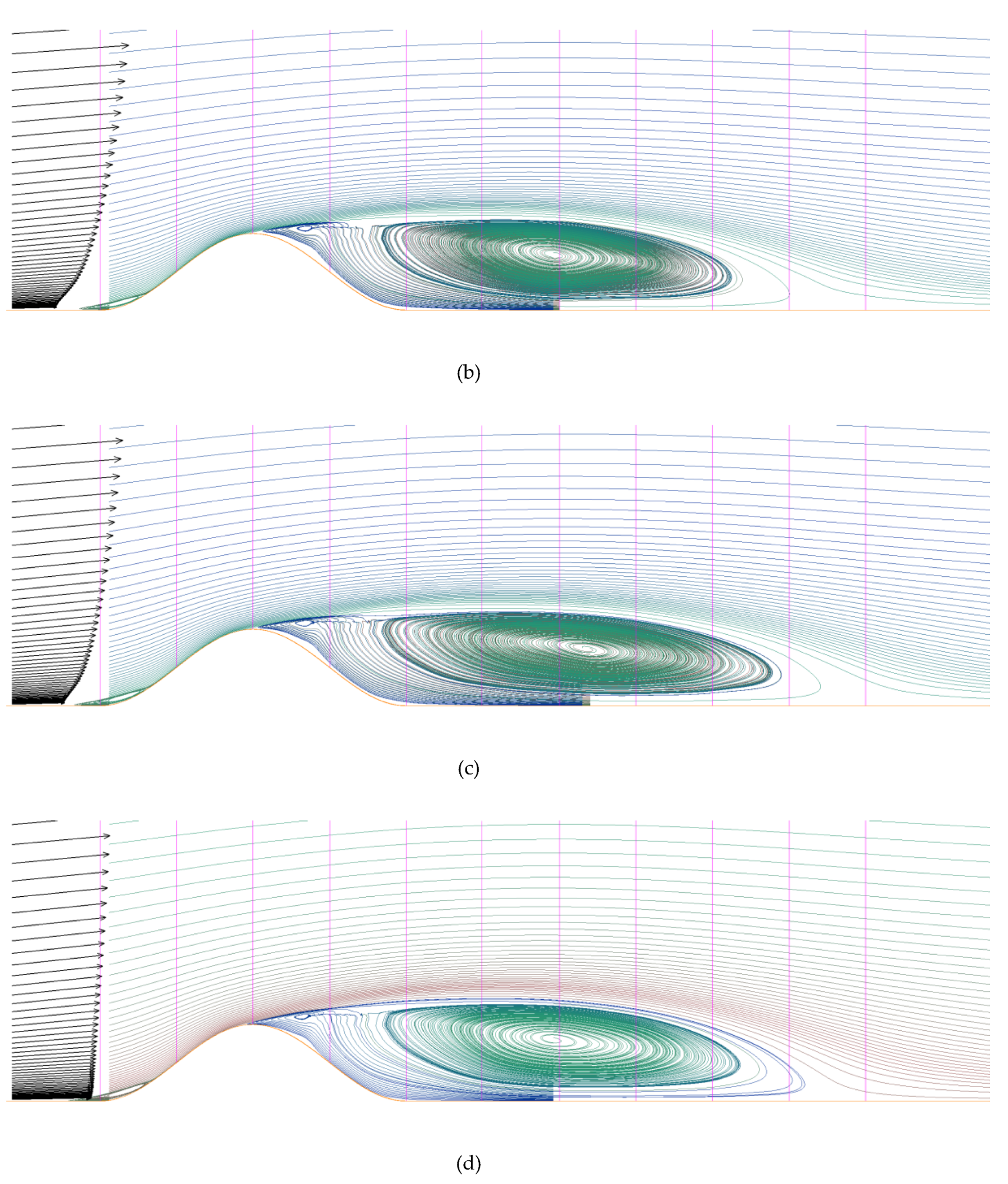
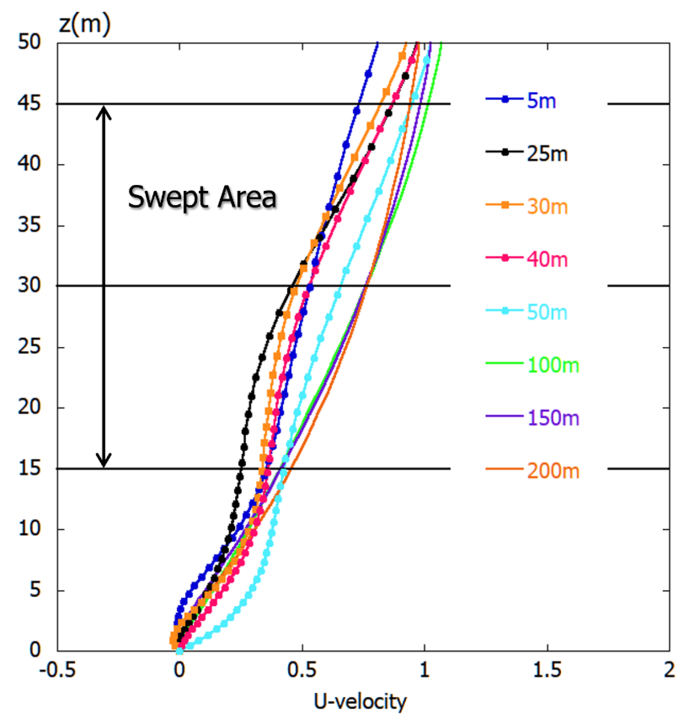
2.5. Results and Discussion

First, as shown in Figure 5, we explain the complex turbulent flow field formed around the two-dimensional ridge model. In the wind tunnel experiment, shown in Figure 5a, the flow field is visualized by the smoke-wire technique. In this method, several wires (0.3 mm nichrome wire) are installed in parallel just upstream of the model with different heights. Oil is applied to the installed wire, and the wire is energized. Finally, we observe the flow field with the smoke generated from the wire. In this wind tunnel experiment, the central section of the model is visualized by illuminating with a 1 kW projector from above the wind tunnel. The wind speed is 1.5 m/s, which is the same condition as the airflow measurement. In particular, in order to pay attention to the behavior of the separated shear layer near the top of the model, the wire height was adjusted so that smoke flows near the surface of the model. The flow past the model is separated near the top of the model. The separated shear layer rolls up into a number of isolated vortices. These isolated vortices merge, one after another. As a result, a separation bubble is formed behind the model. Eventually, a large-scale vortex (transverse vortex) is shed downstream of the model and flows down. Next, we focus on the numerical results—shown in Figure 5b. Similar to the wind tunnel result, shown in Figure 5a, the solitary vortex roll-up from the top of the model, and the subsequent periodic shedding of large vortices can be clearly confirmed.

Using two types of sensor probes, the I-type hot-wire probe and the split film probe, and airflow measurements were performed at a total of nine points on the top and downstream of the two-dimensional ridge model. In this wind tunnel experiment, the mean velocity profiles (U = <u>) and the corresponding standard deviation (σ_u = <u′²>^1/2) in the streamwise direction (x) were evaluated and the results compared. The results obtained are shown in Figure 6 and Figure 7. These figures also show the results of the numerical calculations. In the case of the I-type hot wire probe, only the scalar wind velocity value could be captured, due to the nature of the probe. However, the scalar wind velocity value was treated as a velocity component in the streamwise direction. In both Figure 6 and Figure 7, the horizontal axis of the graph is normalized by the wind velocity aloft U_top at each location. The vertical axis is normalized by the height h of the model. Variable z* on the vertical axis indicates the height from the model surface. Furthermore, the time- and span-averaged flow field (streamlines) obtained by the numerical calculation is shown so that the relationship between the measurement positions and the flow field can be clearly understood.

The mean velocity profiles in Figure 6 show that, at point c on the top of the model, the results of the I-type hot wire probe and the split film probe are almost the same. This is because flow separation does not occur there. At point d, just behind the model, the difference between the results of the I-type hot-wire probe and the split film probe is relatively small because the recirculation region behind the model is not so large.

However, the difference between the two results becomes significant at z*/h < 2 from points e to k downstream of the model. The split film probe results accurately capture the backflow region (negative value) formed behind the model. On the other hand, the I-type hot-wire probe cannot reproduce the negative velocity value associated with the recirculation region behind the model. As a result, at z*/h < 2, the result of the I-type hot wire probe is considerably overestimated compared with the result of the split film probe. At z*/h ≧ 2, the two results are almost the same. Based on these results, the tendency of two kinds of sensor probes in the recirculation region behind the model is clarified. At the same time, the characteristics of the flow past the two-dimensional ridge model are also shown. The behavior of the flow field differs greatly at the boundary of z*/h = 2. That is, the region of z*/h < 2 is strongly affected by the separated flow past the model. On the other hand, at z*/h ≧ 2, the forward flow is the dominant region. It was revealed that the results of the numerical simulation by LES are in better agreement with the wind tunnel experiment using the split film probe than the results of the wind tunnel experiment using the I-type hot wire probe.

Attention should be paid to the vertical profile of the standard deviation, shown in Figure 7. In the mean velocity profile, shown in Figure 6, the wind tunnel experiment results with the I-type hot-wire probe and the split film probe are very different in the wake flow behind the model, including the recirculation region. On the other hand, regarding the standard deviation, both results show similar values at all points and at all height levels. These results are easily imagined because the standard deviation is the amount of deviation (variation component) from the mean value. Based on the above results, the tendency of the airflow measurement with the I-type hot wire probe inserted in a complicated flow field, including the recirculation region, is clarified.

Figure 8 shows a top view of the instantaneous flow pattern around the two-dimensional ridge model. Figure 8a shows the result of the spanwise length of 9 h in the two-dimensional ridge model. Figure 8b shows the result of the spanwise length of 27 h in the two-dimensional ridge model. Figure 8c shows the result of the spanwise length of 54 h. In all the calculation results, the flow field is visualized by the velocity component (U-velocity) in the streamwise direction near the ground and downstream from the two-dimensional ridge model. In addition, three-dimensional streamlines from near the top of the model are drawn. Common to all the calculation results, the three-dimensional structure of the flow downstream of the two-dimensional ridge model is clear. As a result, it is clear that the flow exhibits a complex turbulent field. As the length L in the spanwise direction becomes longer, the presence of rib-like vortex flow structures corresponding to the horizontally beating phenomena in the stationary cylinder wake becomes clear.

Figure 9 shows streamlines for the flow field with temporal and spanwise spatial averaging. The eddies in the downwind flow-separated region formed behind the two-dimensional ridge model are almost the same size in all cases, regardless of the difference in the length L in the spanwise direction.

Figure 10 shows streamlines for numerical results under various inflow shears. Similar to Figure 9, streamlines are drawn based on the flow fields that are time- and spatially-averaged in the spanwise direction. By comparing the results of the four cases, it is clear that the size in the vortex region behind the model is almost the same in all of the calculation results, regardless of the difference in inflow shear.

3. Wind Tunnel Experiments in the Case of Actual Complex Terrain

3.1. Overview of Noma Wind Park in Kagoshima Prefecture

In Figure 11, the wind power plant constructed on the complex terrain targeted in this study is shown. Although the sea surrounds this terrain, it is typical and complex with steep cliff-shaped terrain and an inclination angle of more than 30 degrees on the west side of the cape. The maximum altitude is 143 m. Ten wind turbines owned by Kyushu Electric Power Co., Inc. (Fukuoka, Japan), were installed in this area and were in operation until March 2019. Each wind turbine is rated at 300 kW, and the total output is 3000 kW. As shown in Figure 12, the horizontal distance between wind turbine WT #1 and WT #10 is about 1200 m.

Table 1. Specifications of wind turbines (WTs) at Noma Wind Park.

	WT #1–5	WT #6–10
Output (kW)	300
Generator type	Induction	Synchronous
Cut-in speed (m/s)	3.5	2.5
Rated wind speed (m/s)	14.4	14.0
Cut-out speed (m/s)	24.0	25.0
Rotor diameter (m)	29	30
Tower height (m)	30 (WT #4: 45)	30 (WT #6: 45)

and

Table 2. Wind turbine (WT) hub heights and surface elevations.

	Tower Height (m)	Surface Elevation of Wind Turbine Site (m)
WT #1	30	100
WT #2		92
WT #3		109
WT #4	45	122
WT #5	30	102
WT #6	45	117
WT #7	30	88
WT #8		95
WT #9		92
WT #10		109

show the physical specifications for Noma Wind Park. Figure 13 shows the characteristics of the wind at Noma Wind Park for one year from April 2004 to March 2005, which indicate that this region is affected by prevailing winds from the north. The analysis results, shown in Figure 13, were based on the output values of the propeller-type wind direction and wind speed sensor installed on the wind turbine nacelle, as shown in the dotted line in Figure 14. Figure 15 is a visualization of numerical simulation results targeting the north wind. By observing these results in detail, it is possible to clearly understand how the flow locally changes around the wind turbine. At the same time, it is clearly confirmed that the flow changes three-dimensionally in the sea behind the terrain.

Table 3. Characteristics of the wind at Noma Wind Park for the year from April 2004 to March 2005.

	Hub Height Elevation of the WT Site (m)	Annual Average Wind Speed at Hub Height (m/s)
WT #1	130	6.89
WT #2	122	6.27
WT #3	139	6.94
WT #4	167	7.46
WT #5	132	6.31
WT #6	162	7.02
WT #7	118	5.95
WT #8	125	6.37
WT #9	122	5.92
WT #10	139	6.48
Average value (m/s)		6.56

and Figure 16 show numerical information for the hub height elevation of the WT site (m) and the annual average wind speed at hub height (m/s). Based on these results, there is a strong correlation between the hub height elevation of the WT site (m) and the annual average wind speed at hub height (m/s).

3.2. Scale Model for the Complex Three-Dimensional Terrain

In this study, two types of scale models were created to investigate the effect of terrain irregularities on the airflow characteristics at the hub height of the wind turbine. One is a smooth surface model, as shown in Figure 17a,c. This model is made of polycarbonate and has a smooth shape with no irregularities on the terrain surface. The other is a rough surface model, as shown in Figure 17b,d. This model was made by stacking 1 mm-thick acrylic plates in a staircase pattern. As shown in the photograph in Figure 11, it can be expected that this stepped scale model reproduces the roughness (trees) that uniformly covers the terrain surface. This scale model is generally used in wind tunnel experiments. In this study, for convenience, the former model is called the “scale model without irregularities” and the latter is called the “scale model with irregularities.” On the other hand, in the case of numerical simulation, trees should be better represented by a canopy model (porosity) [23], not by a roughness. The scales of the two types of models created in this study are the same at about 1/2800. Therefore, in both models, the wind turbine hub heights of 30 and 45 m, shown in Table 2, are about 10 and 15 mm in the wind tunnel experiment. In this study, the inflow of 16 wind directions was set every 22.5 degrees for the topographic model, and the mean wind speed at all 10 wind turbine hub height positions was evaluated. Therefore, as shown in Figure 18, we made a turntable that can automatically control the rotation of the scale model by a stepping motor. Figure 18 shows a complex terrain model with no irregularities installed in the wind tunnel. As with the two-dimensional ridge model described above, the scale model was not installed directly on the wind tunnel floor. The terrain was deployed on a 0.115 m turntable that was set on the floor, upstream inside the wind tunnel. Similar to the two-dimensional ridge model, we again focus only on the effect of the shape of the terrain and the presence or absence of surface roughness on the flow field at the hub height of the wind turbine. Therefore, the flow approaching the scale model had a uniform distribution without a velocity shear in the vertical direction.

3.3. Measurement of Airflow at the Hub Height Position of the Wind Turbine Using the I-Type Hot Wire Probe

From the results of the CFD simulation conducted in advance, no flow separation region was observed at each wind turbine hub height position. Therefore, to measure the airflow at the wind turbine hub height, an I-type hot wire probe (KANOMAX Japan, Inc. Model 0251R-T5) and a hot-wire anemometer (KANOMAX Japan, Inc. System 7000, 1011 CTA unit, 1013 linearizer) were used. The settings of offset voltage, gain, cut-off frequency, and the sampling frequency for time-series data acquisition of voltage values were the same as in the case of the two-dimensional ridge model. By using a sampling time (averaging time) of 60 s, the number of data at the hub height position of the wind turbine was 30,000. The inflow wind speed was 1.5 m/s (the rotation speed of the blower is 1190 rpm). The Reynolds number Re (=Uh/ν) based on the maximum model height of about h = 0.6 m was about 6 × 10³.

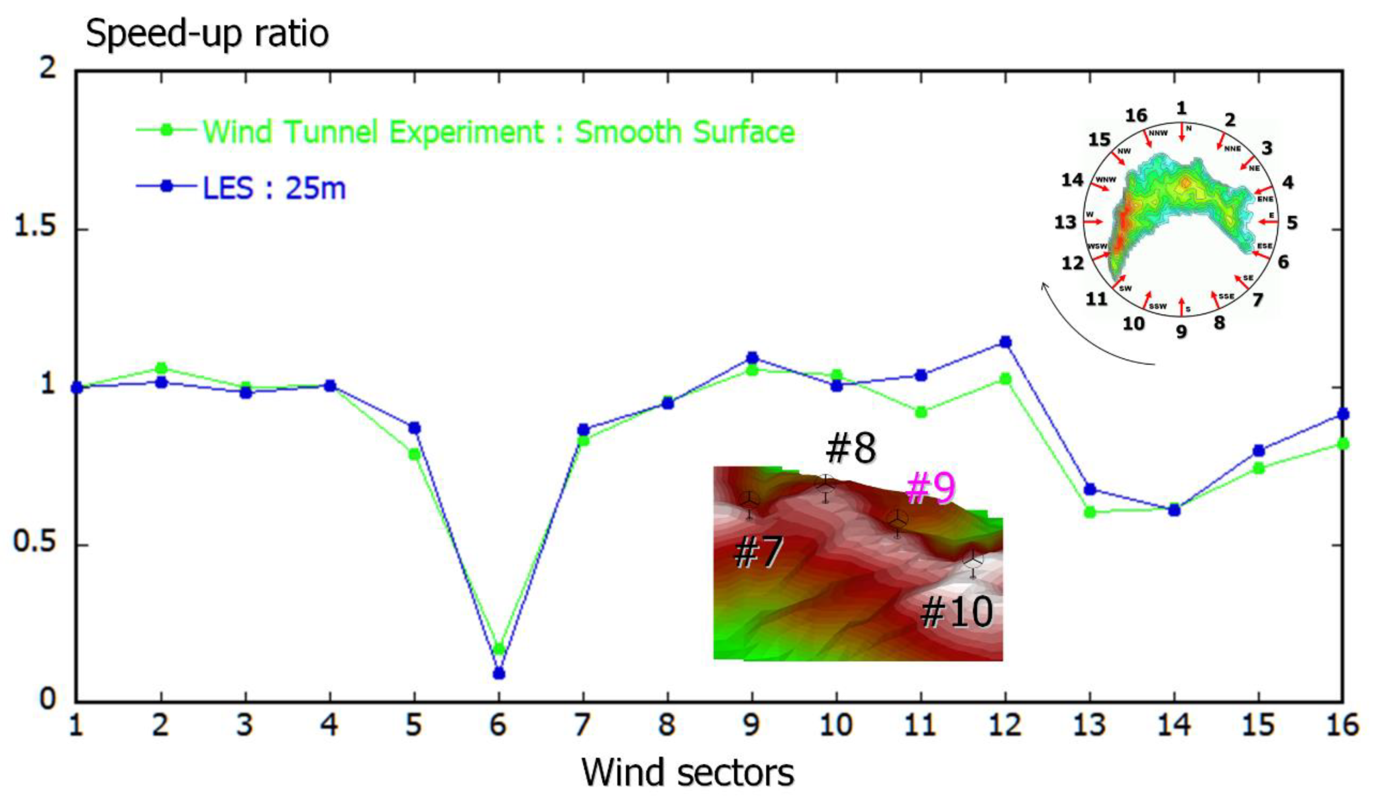
3.4. Results and Discussion

Generally, wind direction should be classed into 16 wind sectors (each sector is 22.5 degrees), as shown in Figure 19. Figure 20 shows a comparison of local speed-up ratios obtained from wind tunnel experiments at wind turbine hub height for 16 wind sectors. Here, the unfilled symbol shows the result of the scale model without irregularities, and the filled symbol shows the results of the scale model with irregularities. Furthermore, the local speed-up ratio at the hub height position of the wind turbine is defined as follows:

local speed-up ratio = mean wind speed at each wind turbine hub height)/mean wind speed at turntable center position (z = 50 mm in the case without a terrain scale model)

(10)

The horizontal axis of the graphs is the wind turbine number, and the vertical axis is the local speed-up ratio defined by Equation (10). Examining Figure 20, it can be seen that the local speed-up ratio may change significantly at the wind turbine position, even in the same wind direction. This indicates that, unlike the flat terrain, the wind speed at the wind turbine hub height position is locally increased or decreased, due to the topographic effect in the complex terrain. It was confirmed that the results of both the scale model without irregularities and the scale model with irregularities showed a similar tendency both quantitatively and qualitatively in all wind directions. Therefore, in the wind tunnel experiments using a 1/2800 scale model, the effect of artificial irregularities on the terrain surface did not significantly appear in the airflow at the hub height of the wind turbine. However, some errors that cannot be ignored in both results can be confirmed. The cause of this might be a measurement error, such as a slight deviation of the probe measurement position. This will be examined further in a later section.

4. Numerical Simulations in the Case of Real Complex Terrain

4.1. Overview of Numerical Simulations

In the previous section, we showed that the wind tunnel experiment using the I-type hot wire probe is an effective method for understanding local speed-up ratios at wind turbine hub height for 16 wind sectors. From here, we next consider the three-dimensional structure of the airflow in the swept area of the wind turbine by using a high-resolution large eddy simulation (LES).

Large eddy simulation (LES) was performed under the same conditions as the wind tunnel experiment for north-westerly wind case, shown in Figure 19. The north-westerly wind is one of the predominant wind directions, as shown in Figure 18. We focused on WT #7 in this wind direction. Because WT #7 is constructed at a slightly lower altitude (see Figure 21). Therefore, WT #7 was expected to be strongly affected by the separated flow generated from the terrain just upstream of the wind turbine. In the present numerical simulations, the smooth surface complex terrain with a horizontal grid resolution of 5 m where the surface roughness does not exist was used as the calculation target, as shown in Figure 22. The number of grid points is 581 (x) × 541 (y) × 71 (z) or about 22 million. The minimum grid width near the topography is 0.425 m. We have confirmed in advance that if the minimum vertical grid width is 1 m or less, there will be no significant difference in the simulation results. As in the wind tunnel experiment, shown in Figure 18, the uniform flow was given for the inflow boundary. Figure 23 shows the representative scales used in the present study. The Adams-Bashforth two-step explicit method was used in the numerical simulation, and the time step was Δt = 1 × 10⁻⁴ h^/U_in. Other simulation methods are the same as in Section 2.4. Flow and turbulence statistics of the numerical simulations were evaluated at a dimensionless time of 50–100.

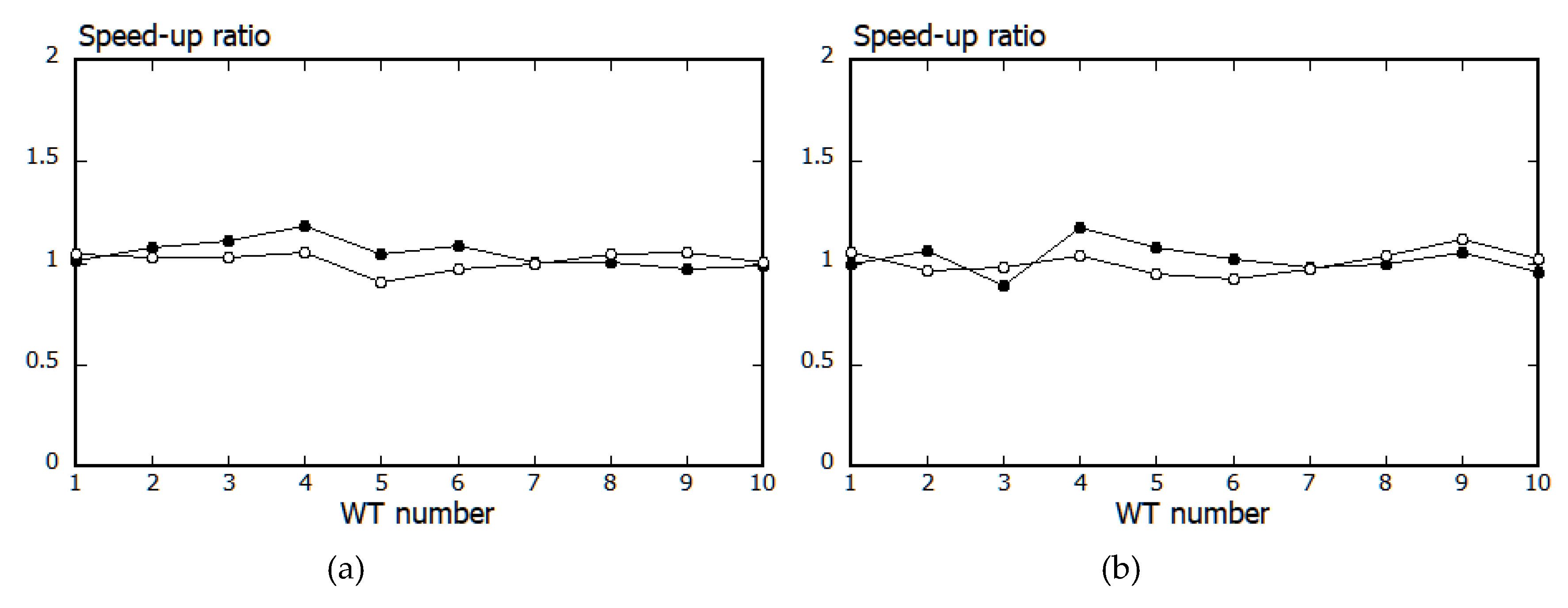
4.2. Results and Discussion

Based on the result of using a 5 m computational grid, we next consider the three-dimensional structure of the airflow in the swept area of WT #7 for north-westerly wind. Effects of horizontal grid resolution on wind behavior formed around WT #7–#10 for 16 wind sectors are summarized in Appendix A. Figure 24 shows the vertical distribution of time-averaged velocity vectors at WT #7. First, we focus on the map view, shown in Figure 24a. As mentioned above, it can be seen that the wind speed of WT #7, surrounded by purple, is clearly lower than that of the other wind turbines. It is understood that the velocity vector at the location of WT #7 is significantly lower than that of other wind turbines. Figure 24b shows an enlarged view of Figure 24a. At the location of WT #7, not only has the wind speed decreased remarkably, but there is also an extremely large velocity shear in the swept rotor area. Next, we focus on the rear view, shown in Figure 24c. Noteworthy here is that the vertical velocity vector in the swept rotor area of the wind turbine is greatly twisted.

Figure 25. shows the time-averaged velocity vectors at the top, bottom, right, and left ends, and the hub center of the WT #7 blades for north-westerly wind. Looking at Figure 25a, two phenomena are confirmed. One is that the directions of the velocity vectors at the blade top end and bottom end are significantly different. Second, the velocity vectors of the blades’ left end, right end, and center are largely shifted to the left. Next, we consider Figure 25b,c. It can be seen that all velocity vectors in the swept rotor area are shifted upwards. In other words, this means that the winds are blowing up into the swept rotor area of the wind turbine under the influence of the topographic effect.

Figure 26 shows the spatial distribution of each velocity component in the swept rotor area of WT #7 for the time-averaged flow field in the case of north-westerly wind. Observing the three numerical results, it is clear that a rotor imbalance in the swept area of the wind turbine was formed.

Finally, we performed parametric studies using various inflow shears, as shown in Figure 27, for the NW case, and numerically examined the effect of the difference in inflow shears on local speed-up ratios. Here, N (shown in Figure 27) indicates the power law index. Figure 28 shows a comparison of local speed-up ratios obtained under various inflow shears for the NW case. The results, shown in Figure A3, indicate that the difference in inflow shears does not significantly affect the local speed-up ratios at the hub height of the wind turbine constructed in the complex terrain.

Generally, the amount of electrical energy generated by a wind turbine, which is defined by the theoretical power curve, is calculated based on the wind speed that penetrates parallel to the ground with respect to the hub center of the wind turbine constructed on flat terrain. However, as mentioned above, careful wind resource assessment is necessary, due to the potential existence of extreme velocity shear and a wind velocity twist in the swept rotor area of the wind turbine over complex terrain. In addition, imbalanced aerodynamic loads in the swept rotor area can lead to wind turbine failure. In addition, it directly affects the life of the wind turbine. There is no doubt that wind resource assessment in complex terrain requires more accuracy than has yet been achieved.

5. Conclusions

Our research group is developing CFD-based software for wind resource and energy production assessments in complex terrain called RIAM-COMPACT, based on large eddy simulation (LES). In order to verify the prediction accuracy of RIAM-COMPACT, we conducted a wind tunnel experiment using a two-dimensional steep ridge model with a smooth surface. In the wind tunnel experiments, airflow measurements were performed using an I-type hot-wire probe and a split film probe that can detect forward and reverse flows. In the mean velocity profile, the wind tunnel experiment results with the I-type hot-wire probe and the split film probe were very different in the region, including the recirculation region behind the model. On the other hand, regarding the standard deviation, both results showed similar values at all points and at all height levels. It was revealed that the results of the numerical simulation by LES are in better agreement with the wind tunnel experiment using the split film probe than the results of the wind tunnel experiment using the I-type hot wire probe. Furthermore, we calculated the two-dimensional ridge model by changing the length in the spanwise direction and discussed the instantaneous flow field and the time-averaged flow field for the three-dimensional structure of the flow behind the model. It was shown that the eddies in the downwind flow-separated region formed behind the two-dimensional ridge model were almost the same size in all cases, regardless of the difference in the length in the spanwise direction. In this study, we also performed a calculation with a varying inflow shear at the inflow boundary. It was clear that the size in the vortex region behind the model was almost the same in all the calculation results, regardless of the difference in the inflow shear.

Next, we conducted wind tunnel experiments on complex terrain. In this study, two types of scale models were created to investigate the effect of irregularities on the terrain surface on the airflow characteristics at the hub height of the wind turbine. One is a smooth surface model with no irregularities on the terrain surface. The other is a rough surface model with stepped irregularities on the terrain surface. Based on the experimental results obtained, the effects of the presence or absence of irregularities on the terrain surface on the flow field at the hub height of the wind turbine were investigated in more detail. In the wind tunnel experiments using a 1/2800 scale model, it was shown that the effect of artificial irregularities on the terrain surface did not significantly appear on the airflow at the hub height of the wind turbine. In order to investigate the three-dimensional structure of the airflow in the swept area in detail, it was clearly shown that LES using a high-resolution computational grid is very effective. In addition, it was shown that the difference in inflow shears does not significantly affect the local speed-up ratios at the hub height of the wind turbine constructed in complex terrain.

References

1. Palma, J.M.L.M.; Castro, F.A.; Ribeiro, L.F.; Rodrigues, A.H.; Pinto, A.P. Linear and nonlinear models in wind resource assessment and wind turbine micro-siting in complex terrain. J. Wind Eng. Ind. Aerodyn. 2008, 96, 2308. [Google Scholar] [CrossRef]
2. Sumner, J.; Watters, C.S.; Masson, C. CFD in Wind Energy: The Virtual, Multiscale Wind Tunnel. Energies 2010, 3, 989–1013. [Google Scholar] [CrossRef] [Green Version]
3. Gopalan, H.; Gundling, C.; Brown, K.; Roget, B.; Sitaraman, J.; Mirocha, J.D.; Miller, W.O. A coupled mesoscale-microscale framework for wind resource estimation and farm aerodynamics. J. Wind Eng. Ind. Aerodyn. 2014, 132, 13. [Google Scholar] [CrossRef]
4. Blocken, B.; Hout, A.V.D.; Dekker, J.; Weiler, O. CFD simulation of wind flow over natural complex terrain: Case study with validation by field measurements for Ria de Ferrol, Galicia, Spain. J. Wind Eng. Ind. Aerodyn. 2015, 147, 43. [Google Scholar] [CrossRef]
5. Murthy, K.S.R.; Rahi, O.P. A comprehensive review of wind resource assessment. Renew. Sustain. Energy Rev. 2017, 72, 1320. [Google Scholar] [CrossRef]
6. Dhunny, A.Z.; Lollchund, M.R.; Rughooputh, S.D.D.V. Wind energy evaluation for a highly complex terrain using Computational Fluid Dynamics (CFD). Renew. Energy 2017, 101, 1. [Google Scholar] [CrossRef]
7. Temel, O.; Bricteux, L.; Beeck, J.V. Coupled WRF-OpenFOAM study of wind flow over complex terrain. J. Wind Eng. Ind. Aerodyn. 2018, 174, 152. [Google Scholar] [CrossRef]
8. Sessarego, M.; Shen, W.Z.; Van der Laan, M.; Hansen, K.; Zhu, W.J. CFD Simulations of Flows in a Wind Farm in Complex Terrain and Comparisons to Measurements. Appl. Sci. 2018, 8, 788. [Google Scholar] [CrossRef] [Green Version]
9. Hewitt, S.; Margetts, L.; Revell, A. Building a Digital Wind Farm. Arch. Comput. Methods Eng. 2018, 25, 879–899. [Google Scholar] [CrossRef] [Green Version]
10. Tang, X.-Y.; Zhao, S.; Fan, B.; Peinke, J.; Stoevesandt, B. Micro-scale wind resource assessment in complex terrain based on CFD coupled measurement from multiple masts. Appl. Energy 2019, 238, 806. [Google Scholar] [CrossRef]
11. El Bahlouli, A.; Rautenberg, A.; Schön, M.; zum Berge, K.; Bange, J.; Knaus, H. Comparison of CFD Simulation to UAS Measurements for Wind Flows in Complex Terrain: Application to the WINSENT Test Site. Energies 2019, 12, 1992. [Google Scholar] [CrossRef] [Green Version]
12. Porté-Agel, F.; Bastankhah, M.; Shamsoddin, S. Wind-Turbine and Wind-Farm Flows: A Review. Bound. Layer Meteorol. 2020, 174, 1–59. [Google Scholar] [CrossRef] [Green Version]
13. Uchida, T. Computational Fluid Dynamics (CFD) Investigation of Wind Turbine Nacelle Separation Accident over Complex Terrain in Japan. Energies 2018, 11, 1485. [Google Scholar] [CrossRef] [Green Version]
14. Uchida, T. LES Investigation of Terrain-Induced Turbulence in Complex Terrain and Economic Effects of Wind Turbine Control. Energies 2018, 11, 1530. [Google Scholar] [CrossRef] [Green Version]
15. Uchida, T. Computational Fluid Dynamics Approach to Predict the Actual Wind Speed over Complex Terrain. Energies 2018, 11, 1694. [Google Scholar] [CrossRef] [Green Version]
16. Uchida, T.; Takakuwa, S. A Large-Eddy Simulation-Based Assessment of the Risk of Wind Turbine Failures Due to Terrain-Induced Turbulence over a Wind Farm in Complex Terrain. Energies 2019, 12, 1925. [Google Scholar] [CrossRef] [Green Version]
17. Uchida, T.; Kawashima, Y. New Assessment Scales for Evaluating the Degree of Risk of Wind Turbine Blade Damage Caused by Terrain-Induced Turbulence. Energies 2019, 12, 2624. [Google Scholar] [CrossRef] [Green Version]
18. Uchida, T.; Ohya, Y. Micro-siting Technique for Wind Turbine Generators by Using Large-Eddy Simulation. J. Wind Eng. Ind. Aerodyn. 2008, 96, 2121. [Google Scholar] [CrossRef]
19. Kim, J.; Moin, P. Application of a fractional-step method to incompressible Navier-Stokes equations. J. Comput. Phys. 1985, 59, 308. [Google Scholar] [CrossRef]
20. Smagorinsky, J. General circulation experiments with the primitive equations: I. Basic experiments. Mon. Weather Rev. 1963, 91, 99. [Google Scholar] [CrossRef]
21. Kajishima, T. Upstream-shifted interpolation method for numerical simulation of incompressible flows. Bull. Jpn. Soc. Mech. Eng. B 1994, 60–578, 3319–3326. (In Japanese) [Google Scholar] [CrossRef]
22. Kawamura, T.; Takami, H.; Kuwahara, K. Computation of high Reynolds number flow around a circular cylinder with surface roughness. Fluid Dyn. Res. 1986, 1, 145–162. [Google Scholar] [CrossRef]
23. Uchida, T. Numerical Investigation of Terrain-Induced Turbulence in Complex Terrain Using High-Resolution Elevation Data and Surface Roughness Data Constructed with a Drone. Energies 2019, 12, 3766. [Google Scholar] [CrossRef] [Green Version]
Figure 1. Effect of topography on wind behavior in complex terrain.
Energies 13 03896 g001
Figure 2. Overview of a thermally stratified wind tunnel.
Energies 13 03896 g002
Figure 3. Two-dimensional ridge model installed in the wind tunnel.
Energies 13 03896 g003
Figure 4. Computational domain, coordinate system, and boundary conditions.
Energies 13 03896 g004
Figure 5. Comparison of the instantaneous flow pattern around a two-dimensional ridge model (side view, y = 0). (a) The wind tunnel experiment shows the smoke-wire technique at a wind speed of 1.5 m/s. (b) Visualization of the numerical simulation and passive particle tracking method.
Energies 13 03896 g005aEnergies 13 03896 g005b
Figure 6. Comparison of nondimensional mean velocity profiles in the wind tunnel experiment and numerical simulation. Numerical flow visualization shows the flow field with time averaging and spatial averaging in the spanwise direction. (a) x = 0h, (b) x = 1h, (c) x = 2h, (d) x = 3h, (e) x = 4h, (f) x = 5h, (g) x = 6h, (h) x = 7h, and (i) x = 8h.
Energies 13 03896 g006aEnergies 13 03896 g006b
Figure 7. Comparison of nondimensional streamwise standard deviation profiles in the wind tunnel experiment and numerical simulation. Numerical flow visualization shows the flow field with time averaging and spatial averaging in the spanwise direction. (a) x = 0h, (b) x = 1h, (c) x = 2h, (d) x = 3h, (e) x = 4h, (f) x = 5h, (g) x = 6h, (h) x = 7h, and (i) x = 8h.
Energies 13 03896 g007aEnergies 13 03896 g007b
Figure 8. Instantaneous flow pattern around a two-dimensional ridge model (streamlines, top view): (a) L = 9 h, (b) L = 27 h, and (c) L = 54 h.
Energies 13 03896 g008aEnergies 13 03896 g008b
Figure 9. Streamlines for flow field with temporal and spanwise spatial averaging: (a) L = 9 h, (b) L = 27 h, and (c) L = 54 h.
Energies 13 03896 g009aEnergies 13 03896 g009b
Figure 10. Streamlines for the flow field with temporal and spanwise spatial averaging. Numerical results under various inflow shears: (a) Power-law index N = 4, (b) power-law index N = 7, (c) power-law index N = 10, and (d) uniform flow.
Energies 13 03896 g010aEnergies 13 03896 g010b
Figure 11. Complex terrain targeted in this study and ten wind turbines constructed at the Noma Wind Park.
Energies 13 03896 g011
Figure 12. Map of elevations at the wind farm (WF).
Energies 13 03896 g012
Figure 13. Characteristics of the wind at Noma Wind Park, WT #4, for the year from April 2004 to March 2005: (a) Occurrence frequency (%) and (b) annual average wind speed (m/s). The time-series data interval used to construct the plots was 1 minute.
Energies 13 03896 g013
Figure 14. Propeller vane anemometer mounted on a wind turbine nacelle (indicated by the dotted line).
Energies 13 03896 g014
Figure 15. Numerical flow visualization over Noma Wind Park by using the passive particle tracking method.
Energies 13 03896 g015
Figure 16. Relationship between the hub height elevation and annual average wind speed at hub height for the year from April 2004 to March 2005.
Energies 13 03896 g016
Figure 17. Comparison of whole and enlarged views of the scale model: (a,c) Scale model without irregularities made from polycarbonate, and (b,d) scale model with irregularities made by stacking 1 mm-thick acrylic plates.
Energies 13 03896 g017
Figure 18. Complex three-dimensional terrain model without irregularities installed in the wind tunnel.
Energies 13 03896 g018
Figure 19. Sixteen wind sectors (each sector is 22.5 degrees).
Energies 13 03896 g019
Figure 20. Comparison of local speed-up ratios obtained from wind tunnel experiments at wind turbine hub height: (a) N, (b) NNE, (c) NE, (d) ENI, (e) E, (f) ESE, (g) SE, (h) SSE, (i) S, (j) SSW, (k) SW, (l) WSW, (m) W, (n) WNW, (o) NW, and (p) NNW. The unfilled symbol shows the result of the scale model without irregularities, and the filled symbol shows the result of the scale model with irregularities.
Energies 13 03896 g020aEnergies 13 03896 g020bEnergies 13 03896 g020c
Figure 21. Terrain shapes passing through WT #7 for north-westerly wind.
Energies 13 03896 g021
Figure 22. Smooth surface complex terrain with a horizontal grid resolution of 5 m.
Energies 13 03896 g022
Figure 23. Representative scales used in the present study.
Energies 13 03896 g023
Figure 24. Vertical distribution of the time-averaged velocity vectors at WT #7. for north-westerly wind: (a) Oblique map view, (b) side view, and (c) rear view. This flow visualization is based on the numerical results using a 5 m grid.
Energies 13 03896 g024aEnergies 13 03896 g024b
Figure 25. Vertical distribution of time-averaged velocity vectors at WT #7 for north-westerly wind: (a) Rear view from slightly above, (b) rear view, and (c) side view. This flow visualization is based on the numerical results using a 5 m grid.
Energies 13 03896 g025
Figure 26. Spatial distribution of each velocity component in the swept rotor area of WT #7 for the time-averaged flow field in the case of north-westerly wind: (a) Streamwise velocity component, (b) spanwise velocity component, and (c) vertical velocity component.
Energies 13 03896 g026
Figure 27. Various inflow shears investigated in this study.
Energies 13 03896 g027
Figure 28. Comparison of local speed-up ratios obtained under various inflow shears for north-westerly wind.
Energies 13 03896 g028