Small-Scale Desalination Plant Driven by Solar Energy for Isolated Communities

Abstract

In the last years, an increasing number of countries has been affected by water shortage. Seawater desalination driven by solar energy, which is usually available in arid regions, might be a solution to satisfy the freshwater demand. In this study, the feasibility of a stand-alone multi-effect desalination (MED) plant driven by solar energy for an isolated community was studied. The system was made up of a solar field, a MED unit, and a thermal storage that mitigated solar energy fluctuations. Simulations with different top brine temperature and inclination and number of the solar panels were carried out in Matlab and Aspen Plus on an hourly basis by considering one typical meteorological year for ambient temperature and solar radiation. Two different sources of electrical energy were considered: A photovoltaic (PV) field and a diesel generator. The results were compared from an energetic and economic point of view, by considering the adoption of plastic as a material for MED heat exchangers. The maximum water production was obtained with December as the design month. Polytetrafluoroethylene heat exchangers allowed the cost of water to be reduced up to 9.5% compared to conventional exchangers. The lowest cost of water (7.09 $/${\mathrm{m}}^3$) was obtained with September as the design month and a tilt angle of 45° with the PV field as the electrical power source.

1. Introduction

Water is an essential element for human life. The growth of the world population and ever higher standard of life are causing an exponential increase of freshwater demand. These factors, coupled with the climate changes that the world is witnessing, accentuates the freshwater shortage problem. More and more countries are affected by water stress or scarcity. Seawater desalination is a solution to overcome this problem since many arid regions are situated near the coast. The installed capacity of desalination plants has been increasing very fast and it has reached 97.4 million cubic meters per day [1].

Water desalination processes can be divided in membrane and thermal processes. The most diffuse membrane processes are reverse osmosis and electrodialysis. The main thermal processes are multi-stage flash (MSF), multi-effect desalination (MED), and vapor compression distillation. Membrane processes, especially reverse osmosis, are the fastest growing [2] and most widespread technology. They generally show better thermodynamic performance than thermal technologies. On the other side, membrane technologies have a higher electrical energy consumption. Furthermore, they have a lower recovery rate, and hence higher specific energy consumption in the case of high-salinity feed water [3].

Among desalination processes, the interest in MED thermal process is growing due to high thermal efficiency, low electrical energy consumption, and low operation cost [4]. The maximum temperature of the first effect generally does not exceed 80 °C, thus enabling the operation with low-temperature heat sources. Moreover, MED has more stability at partial load conditions than MSF [5] and it has been found to be more efficient than MSF in terms of energy consumption [6]. Desalination systems integrated with renewable energies were reviewed by Alkaisi et al. [7]. They considered solar energy as the most applicable source since it can produce both the heat and electricity required by all desalination processes. Typically, the countries affected by water scarcity have a great availability of solar energy and many researchers have studied the integration of MED plants and solar plants. El-Nashar [8] compared three different systems for small-scale MED desalination: a conventional system using a steam and diesel generator; a solar-assisted system in which solar collectors provided the thermal energy and a diesel generator provided the pumping power; a solar system in which the thermal energy was supplied by solar collectors and pumping power by solar photovoltaic (PV). His results confirm that even if solar energy cannot currently compete with fossil energy, the use of solar energy can be an attractive alternative in many remote, arid and sunny areas of the world due to the higher cost of fuel transportation [8].

Saldivia et al. [9] studied a desalination system made up of a MED plant, a solar generation plant with parabolic collectors, a storage tank, and a steam generator. They analyzed the coupling between the solar generation plant and the MED. The implications for their joint behavior on the performance of the whole system were analyzed through simulations based on hourly meteorological data [9]. They found that the external steam temperature and maximum allowed concentration of rejected brine were the key parameters.

Kazemian et al. [10] performed the optimization of multi-effect desalination plant studying the effects of feed water flow rate, temperature of seawater, numbers of effects, temperature differences of preheaters, and the outlet pressure. Their results provide a guidance to find suitable thermodynamic conditions at different situations for which the plant would operate close to its optimum condition [10].

In the last years, several studies focused on the possibility of using plastic heat exchangers [11,12,13]. They have lower cost, lighter weight, higher chemical resistance to acids, oxidizing agents and many solvents, and higher erosion resistance [11], this requiring less maintenance in comparison to conventional metallic exchangers. These advantages can outweigh the drawback of a lower conductivity that implies higher heat transfer areas and consequently, a higher MED capital cost.

In this work, a stand-alone MED plant powered by a solar field with evacuated tube collectors located in a small town near the coast in the Western Sahara was studied. This plant should compensate the limited local freshwater availability. A thermal storage was added to mitigate the daily solar fluctuations and grant a continuous operation of the MED. The storage was modeled as a stratified tank to simulate the temperature in the tank across one year. This differs from other studies in which the storage is simply modeled as a full-mix tank.

The energy and economic analysis has been conducted through simulations in Matlab [14] and Aspen Plus [15] at different values of the MED top brine temperatures (TBT) plant, tilt angle of the solar collectors, and design month.

Two cases were considered to produce the electrical power required by the plant: A PV field and a diesel generator. These two cases were compared in terms of production cost of water (COW). Both conventional and polytetrafluoroethylene (PTFE) heat exchangers were considered and compared in terms of COW.

The suitability to choose the lowest TBT (50 °C) for the MED has been shown in energy and COW terms. The models of the solar field and storage tank were replicated from the literature, while a detailed model of the desalination unit was realized in Aspen Plus. The study allows for the definition of a methodology to design isolated solar desalination plants for remote areas by proposing various typologies of electric supply, materials for MED heat exchangers, and solar field parameters. Particularly, the adoption of plastic heat exchangers is an important factor to reduce water cost in small-scale thermodynamic desalination systems.

2. Materials and Methods

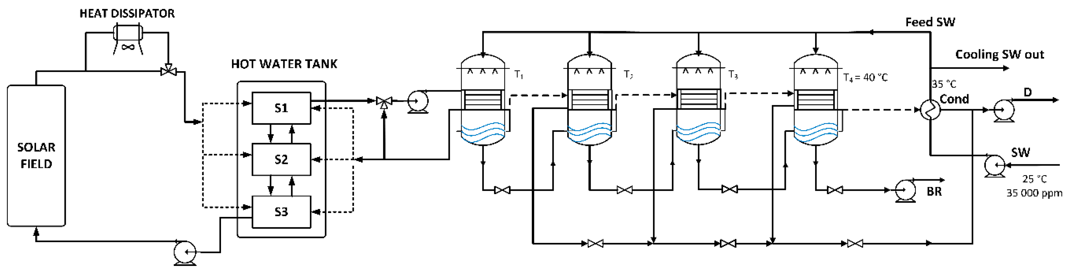
The system investigated is made up of a solar field, a thermal energy storage (TES), and a MED plant as shown in Figure 1. The solar field, operated with water, provided the thermal energy to the desalination unit. A TES was interposed between the two systems to guarantee a continuous operation of the desalination unit. A four-stage parallel/cross MED was considered.

With regard to the climatic conditions and the freshwater requirement, reference was made to Lemseid, a small town near the coast in the Western Sahara, since it was considered significant for the characteristics of the studied technology. Lemseid has a population of about 570 people [16]. The desalination plant might compensate for the limited local freshwater availability. The nominal daily production rate of the MED plant was fixed at the local daily basic access demand of freshwater. A freshwater consumption of 0.02 ${\mathrm{m}}^3/\mathrm{d}$ per capita is considered as a basic access [17]. On the basis of the number of inhabitants, the local daily basic access demand of freshwater was estimated to be 11.4 ${\mathrm{m}}^3/\mathrm{d}$.

The system was studied for different values of some significant parameters: The TBT of the MED plant, the inclination of solar collectors, and the month taken as reference to design the solar field.

The TBT of the MED plant—the temperature of the brine at the 1st effect inlet—can have a significant role in determining the annual operating hours: Lower TBTs allow for the use of heat at lower temperatures, thus increasing the operating time. In addition, low TBTs increase the MED performance ratio, thus reducing the specific heat required by the process [18]. On the other hand, lower TBTs decrease temperature differences between one effect and the following. This increases the cost of the plant because of the higher surface required to transfer the same amount of heat. For these reasons, the MED plant was investigated by considering three different values of TBT—60, 55, and 50 °C—to understand how TBT affects both the operating hours and the water production cost, with the temperature of the last effect fixed at 40 °C. TBTs lower than 50 °C were not considered: The minimum temperature difference between one effect and the following is 2.5 °C to take into account the boiling point elevation and a minimum temperature difference to allow the heat transfer.

The size of the solar field was determined by considering the daily thermal energy required by the MED plant in the average day of a month chosen as a reference and given the tilt angle of the collectors (β). In this way, the number of collectors was determined once given the TBT, β, and design month.

The choice of the design month had a great influence on the number of solar collectors required, and consequently on the capital cost of the solar field. For example, the choice of a cold month like December as the design month led to a high number of collectors and capital cost, but also to a high annual utilization factor ($f_u$) and freshwater production. Therefore, three different design months were considered: March, September, and December. Summer months were not investigated as the resulting solar field would be small and $f_u$ would be very low, making the plant unable to provide freshwater for most of the year.

Each month has an optimal value of tilt angle (β) that maximizes the solar irradiance in that month. Generally, this value of β is different from the value maximizing the solar energy collection of the whole year. For this reason, four different values of β were considered (25°, 35°, 45°, 55°), chosen on the basis of a preliminary analysis carried out according to the Liu–Jordan method [19].

Annual simulations were developed for each combination of TBT, design month, and β, resulting in 36 (3 × 3 × 4) total cases. The simulations of the solar field and the thermal storage were performed in the Matlab [14] with hourly weather data of temperature and solar irradiance from the PVGIS (Photovoltaic Geographical Information System) database [20]. These data were linearly interpolated to obtain a continuous function of boundary conditions. A time step of 6 min was used for the solution of the differential equations to have a more accurate estimation of the temperature profiles in the storage. For the MED plant, an Aspen Plus [15] model was developed as in [21], and the required thermal power and the produced amount of water were imported in the Matlab model as a look-up table.

The main variables and parameters adopted to study the system are summarized in

Table 1. Main variables and parameters of the system.

Input Variables	Values
TBT	50, 55, 60 (°C)
design month	Dec, March, Sept
β	25, 35, 45, 55 (°)
exchangers material of construction	conventional, PTFE
electric supply	Diesel generator, PV field
Constant Parameters	Values
MED nominal desalted water production rate seawater temperature and salinity	11.4 ${\mathrm{m}}^3/\mathrm{d}$ 25 °C and 35,000 ppm

.

The aim of the simulations is to determine the best configuration in terms of yearly water production and cost of water as a function of solar parameters, exchangers material of construction, and electric supply.

2.1. MED Plant

The desalination plant is a parallel/cross flow MED with 4 effects, shown in the right side of Figure 1. In this configuration, feed seawater was split into four streams and sprayed on the heat exchanger surface of each effect. Here, feed seawater partly evaporated by exploiting the heat of the complete condensation of the vapor produced in the previous effect. In the case of the first effect, the heat was provided by the sensible heat of the water from the thermal energy storage. The brine collected at the bottom of each effect flowed into the subsequent effect where it partly flashed due to the lower pressure. The vapor produced in the last effect was completely condensed in the final condenser by seawater. A part of the seawater exiting this condenser at 35 °C was used as feed seawater, whereas the other part was rejected back to the sea. The brine of the last effect was discharged into the sea.

The temperature of the brine in the last effect (bottom brine temperature) was fixed to 40 °C. The temperature difference between each effect and the following was assumed to be the same. Consequently, the temperature of each effect k is:

$$T_k=\mathrm{TBT}-\frac{(\mathrm{k}-1)}{3}(\mathrm{TBT}-40°\mathrm{C}).$$

(1)

The inlet temperature of the water from the storage was controlled at a constant value by mixing part of the water from the outlet of the brine heater with the flow from the thermal storage. The inlet temperature set point was fixed at TBT + 15 °C. The mass flow of the hot water entering the first effect was therefore determined by the heat required by the MED plant through the energy balance and was imposed to be constant during the operation; the outlet temperature of the MED was constant and the part load operation of the desalination unit was avoided.

A maximum salt concentration of 95% of the solubility was imposed to the brine at the exit of each effect as in [21]. In this way the recovery ratio (RR) was maximized as shown in [21]. This condition was achieved by imposing different mass flow rates of feed seawater in each effect. The maximum salt concentration in the seawater was limited by the calcium sulphate precipitation and it was a decreasing function of the temperature. The analytical expression of the maximum salt concentration is provided by [18]:

$$\tilde{S}(T\left[°\mathrm{C}\right])=4.71166\times {10}^{-3}{T}^4-1.74116T^3+253.842T^2-17922.8T+565818\left[\mathrm{ppm}\right].$$

(2)

One of the parameters commonly used in literature to evaluate better the performance of desalination processes is the performance ratio (PR), defined as the ratio between desalted water mass flow rate obtained in the process (${\dot{V}}_D$) multiplied by pure water latent heat of evaporation at 70 °C ($\mathsf{\Delta }{h}_{ev}$ = 2.33 MJ/kg, constant) and the external heat ($\dot{Q}$) supplied to the plant [22].

$$PR=\mathsf{\Delta }{h}_{ev}{\dot{V}}_D/\dot{Q}$$

(3)

$PR$ is a dimensionless parameter and expresses the ratio between the produced desalted water rate and the equivalent mass flow rate of condensing saturated water vapor at 70 °C required for its production.

The MED plant works at nominal conditions and it is turned off when the temperature of the hot water goes below the required inlet temperature. The start-up of the plant occurs when the average temperature of the water in the storage is higher than a fixed value defined by Equation (4):

$$(T_{st,max}+T_{st,min})/2>\mathrm{TBT}+\mathsf{\Delta }T,$$

(4)

where $\mathsf{\Delta }T$ = 32.5 °C is a good compromise between the need of avoiding frequent plant on/off and a proper exploitation of the thermal storage.

The utilization factor ($f_u$), directly proportional to the annual freshwater production, was calculated for each annual simulation as:

$$f_u=\frac{\left[annualMEDequivalenthours\right]}{8760h}.$$

(5)

Both conventional and polytetrafluoroethylene (PTFE) heat exchangers for the MED evaporators were considered. The heat transfer surface areas of the conventional heat exchangers were estimated assuming an overall heat transfer coefficient ($\mathrm{U}$) for each heat exchanger. An overall heat transfer coefficient of 650 $W/(m^{2}K)$ was derived from Sinnott et al. [23] for the first effect in case of conventional exchangers. This approach was followed by other authors in the literature [24]. The values of the overall heat transfer coefficient for the other heat exchangers and for the condenser were calculated from the correlation reported in [18], respectively for fouled evaporator and fouled condenser:

$${\mathrm{U}}_{ev,conv}(T)=1939.4+1.40562T-2.07525\times {10}^{-2} T^2+2.3186\times {10}^{-3} T^3\left[\mathrm{W}/({\mathrm{m}}^2\mathrm{K})\right]$$

(6)

$${\mathrm{U}}_{cond,conv}(T)=1617.5+0.1537T+0.1825T^2-8.026\times {10}^{-5}{T}^3=1910\left[\mathrm{W}/({\mathrm{m}}^2\mathrm{K})\right].$$

(7)

These overall transfer coefficients refer to the conventional (conv) metallic heat exchangers in copper alloy. PTFE heat exchangers have lower overall transfer coefficients than alloy. Song et al. [12] found an overall heat transfer coefficient of 826 W/$({\mathrm{m}}^2\mathrm{K})$ for PVDF hollow fiber evaporators.

Therefore, an additional thermal resistance of $7.5\times {10}^{-4}{\mathrm{m}}^2\mathrm{K}/\mathrm{W}$ was estimated and used to determine the heat transfer coefficients of PTFE exchangers for each heat exchanger and for the 3 different TBTs from the corresponding conventional heat transfer coefficient. The overall heat transfer coefficients are reported in

Table 2. Overall heat transfer coefficients [W/(m² K)].

TBT	Exchanger	${\mathbf{U}}_{\mathbf{e}\mathbf{v} 1}$	${\mathbf{U}}_{\mathbf{e}\mathbf{v} 2}$	${\mathbf{U}}_{\mathbf{e}\mathbf{v} 3}$	${\mathbf{U}}_{\mathbf{e}\mathbf{v} 4}$	${\mathbf{U}}_{\mathbf{c}\mathbf{o}\mathbf{n}\mathbf{d}}$
60 °C	Conventional	650	2307	2195	2111	1910
	PTFE	436	840	825	812	781
55 °C	Conventional	650	2248	2172	2111	1910
	PTFE	437	837	826	817	785
50 °C	Conventional	650	2195	2150	2111	1910
	PTFE	437	830	823	817	785

.

The heat transfer area $(A_i)$ of each heat exchanger was calculated as the ratio between the heat exchanged and the product of the average logarithmic mean temperature difference (${\mathsf{\Delta }\mathrm{T}}_{\mathrm{ml}}$) and the overall heat transfer coefficient $({\mathrm{U}}_{\mathrm{i}})$:

$$A_i={\dot{Q}}_i/({\mathrm{U}}_{\mathrm{i}}{\mathsf{\Delta }\mathrm{T}}_{\mathrm{ml}\mathrm{i}}).$$

(8)

2.2. Solar Field

The solar field consists of evacuated tube collectors connected in series and parallel according to the manufacturer’s instruction [25], with a maximum of 6 collectors in series. Evacuated tube collectors (CSV 35 R [25]) were chosen; their main characteristics are shown in

Table 3. Main characteristics of solar collectors CSV 35 R [25].

Characteristic	Value	Units
total area	3.91	${\mathrm{m}}^2$
exposed area	3.43	${\mathrm{m}}^2$
optical efficiency, ${\mathsf{\eta }}_0$	0.70	-
thermal dispersion factor ${\mathsf{\alpha }}_1$	1.15	$\mathrm{W}/({\mathrm{m}}^2\mathrm{K})$
thermal dispersion temperature dependence factor, ${\mathsf{\alpha }}_2$	0.011	$\mathrm{W}/({\mathrm{m}}^2{\mathrm{K}}^2)$
n° vacuum tubes	20	-

.

The number of collectors ($N_{coll}$) was determined as a function of the TBT, the design month, and the tilt angle to produce the thermal energy required by the MED in the average day of the month $(\dot{Q})$. The daily solar energy captured per square meter of collector’s exposed area, $q_u$ $\left[\frac{\mathrm{Wh}}{{\mathrm{m}}^2\mathrm{d}}\right]$, was determined as:

$$q_u={{\displaystyle \sum }}_{k=1}^{24}{\eta }_{coll,k}{G}_{t,k};{\eta }_{coll,k}={\eta }_0+{\alpha }_1\frac{(T_m-T_{a,k})}{G_{t,k}}-{\alpha }_2\frac{{(T_m-T_{a,k})}^2}{G_{t,k}}$$

(9)

where $G_{t,k}$ is the hour solar radiation incident on the collectors’ surface.

The required number of collectors was:

$$N_{coll}=A_{tot}/A_{coll};A_{tot}=\dot{Q}\left[W\right]·24\left[\frac{h}{d}\right]/q_u.$$

(10)

2.3. Thermal Energy Storage

The TES consists in a water tank at atmospheric pressure. It is the simplest way to storage solar thermal energy. The tank is modeled as a stratified tank with the multi-node approach described in [26]. In this model, the tank was divided into 3 sections (nodes), with mass and energy balances written for each section. The result was a set of 6 differential equations that can be discretized and solved for the temperatures of the 3 nodes as functions of time according to the finite volume approach. The water mass flow rate from the solar collectors and that coming back from the MED entered in the storage at the node with the nearest value of the temperature. Each node exchanged mass and energy with the near ones. The temperature trends of the three nodes during a year and, consequently, the annual operability of the entire system was obtained by simulating this model coupled with solar field equations in transient conditions.

The storage volume was 50 ${\mathrm{m}}^3$ to allow the MED operation during the night. A maximum temperature of 95 °C was imposed. A heat dissipator was included in the system to prevent overheating.

2.4. Electrical Generation

Electrical generation is required for water pumping. Two different cases were considered. In the first case a PV plant with a battery provided all the electrical energy required. In the second case, a diesel generator produced the required electrical energy. The electrical power demand $(P_{el,req})$ was determined as the sum of the power required by the MED plant ($P_{el,MED}$) and the power required for the water circulation in the solar field $(P_{el, circ})$:

$$P_{el,req}=P_{el,MED}+P_{el,circ}.$$

(11)

The electrical power required by the MED plant $(P_{el,MED})$ was calculated by assuming a specific electrical energy consumption $(e{c}_{el,MED})$ of $2\mathrm{kWh}/{\mathrm{m}}_{\mathrm{D}}^3$ [27]:

$$P_{el,MED}=e{c}_{el,MED}\frac{{\dot{V}}_D}{24h/d}\left[{\mathrm{kW}}_{\mathrm{el}}\right].$$

(12)

The power required for the water circulation was calculated through the correlation [8]:

$$P_{el, circ}=2.691\times {10}^{-2} {(0.03 A_{tot, coll})}^{1.13} \left[{\mathrm{kW}}_{\mathrm{el}}\right].$$

(13)

Therefore, the total electrical energy consumption $(e{c}_{el,tot})$ per cubic meter of freshwater was:

$$e{c}_{el,tot}\left[\frac{\mathrm{kWh}}{{\mathrm{m}}_{\mathrm{D}}^3}\right]=e{c}_{el,MED}+\frac{P_{el,circ}}{24h{\dot{V}}_D} .$$

(14)

The PV installed power ($P_{PV}$) of the PV system (PV field + batteries) was calculated as:

$$P_{PV}=\frac{P_{el,req}·24h}{0.8K_{E/P}} with K_{E/P}=5.3\frac{\mathrm{kWh}}{{\mathrm{kW}}_{\mathrm{p}}}.$$

(15)

2.5. Economic Analysis

El-Nashar [8] reports a cost correlation for the specific capital cost of a MED plant as a function of the TBT, the number of effects, and the daily desalted water production (in [${\mathrm{m}}^3/\mathrm{d}$]):

$$C_{cap,MED conv}=5.1205\times {10}^6 {(\frac{{\dot{V}}_D}{2500})}^{0.7}{(\frac{N_{eff}}{8})}^{0.5}{(\frac{70}{\mathrm{TBT}})}^{0.47}.$$

(16)

This cost correlation was multiplied by the cost actualization factor based on the Chemical Engineering Plant Cost Index (CEPCI) to be referred to the year 2018 and used to determine the capital cost of the MED in the case of conventional heat exchangers. The capital cost of the evaporators in both conventional and PTFE materials was calculated through Equation (17) [28]. The material factors $(F_M)$ adopted were respectively 1.7 (copper alloy) for conventional exchangers and 0.2 for the PTFE exchangers. This latter value was chosen because, as reported in [11], the plastic is 1/5 less expensive than carbon steel (material that has been taken as a reference material in [28]).

$$\begin{array}{l}{C}_{cap,evap,conv/PTFE}=1.18\times (B_1+B_2{F}_M{F}_P)\times \\ {\displaystyle {\displaystyle \sum }_{i=1}^4}exp\left\{11.0545-0.9228\ln (10.7639A_{i, conv/PTFE})+0.09861{\left[\ln (10.7639A_{i,conv/PTFE})\right]}^2\right\} \end{array}$$

(17)

with $B_1=1.63,B_2=1.66,F_P=1.25$.

In the case of conventional exchangers, the capital cost of the evaporators was assumed to be 40% $(f_{HEX}=0.4)$ of the MED plant capital cost and the remaining 60% was assumed to be not dependent on the material of the heat exchangers [29].

With these assumptions, the capital cost of the MED plant with PTFE heat exchangers $C_{cap,MED PTFE}$ was:

$$C_{cap,MEDPTFE}(\mathrm{TBT})=K_M(\mathrm{TBT})C_{cap,evap,PTFE}(\mathrm{TBT})+(1-f_{HEX})C_{cap,MEDconv}$$

(18)

where $K_M$ is a multiplying factor defined as:

$$K_M(\mathrm{TBT})=C_{cap,MEDconv}(\mathrm{TBT})/(C_{cap,evapconv}(\mathrm{TBT})1/f_{HEX})$$

(19)

The cost of maintenance was assumed to be the 2.5% of annualized $C_{cap,MED}$.

The brine disposal cost in $(\$/m_D^3)$ is calculated as in [27]:

$${\tilde{c}}_{br disp}=1.5\times {10}^{-3} ·(1/\mathrm{RR}-1).$$

(20)

The cost of the solar field was calculated as:

$$C_{cap,sf}=c_{ETC} ·N_{coll} ·A_{coll};c_{ETC}=320\$/{\mathrm{m}}^2.$$

(21)

The cost of the water thermal storage was calculated as ([8]):

$$C_{cap,st}=c_{st} V_{st} \mathrm{with}{c}_{st}\left[\frac{\$}{m^3}\right]=456.6 {(\frac{V_{st}}{300})}^{0.6}$$

(22)

and multiplied by the CEPCI index to be referred to the year 2018.

The cost of the PV system (PV field + batteries) was calculated as:

$$C_{cap,PV}=c_{PV} · P_{PV}+C_{batt};c_{PV}=2 \$/\mathrm{W};{\mathrm{C}}_{\mathrm{batt}}=50 kWh · 300 \$/\mathrm{kWh}.$$

(23)

The cost of the diesel generator was calculated as:

$$C_{cap,\mathrm{dies}}=125\frac{\$}{\mathrm{kW}}·P_{el,req}.$$

(24)

By assuming a cost of the fuel ($c_f$) of 1.026 $/L and a fuel consumption ($\mathrm{fc}$) of 0.3 $\mathrm{L}/{\mathrm{kWh}}_{\mathrm{el}}$, the annual fuel cost was:

$${\overline{C}}_{fuel,ann}\left[\frac{\$}{\mathrm{y}}\right]=e{c}_{el,tot}(365\frac{d}{y}·{\dot{V}}_D·f_u){\mathrm{fc}\mathrm{c}}_{\mathrm{f}}.$$

(25)

Finally, the cost of the water was calculated as:

$$\mathrm{COW}\left[\frac{\$}{{\mathrm{m}}_{\mathrm{D}}^3}\right]=\frac{\mathrm{CFR}(C_{cap,\mathrm{MED}}+C_{cap,\mathrm{sf}}+C_{cap,\mathrm{st}}+C_{cap,\mathrm{PV}/\mathrm{dies}})+{\overline{C}}_{maint,ann}+{\overline{C}}_{fuel,ann}}{f_u{\dot{V}}_D\left[{\mathrm{m}}^3/\mathrm{d}\right]365[\mathrm{d}/\mathrm{y}]}+{\tilde{c}}_{brdisp}$$

(26)

where $\mathrm{CRF}=\mathrm{IR}{(1+\mathrm{IR})}^{\mathrm{N}}/\left[{(1+\mathrm{IR})}^{\mathrm{N}}–1\right]$ is the capital recovery factor or amortization factor, $\mathrm{IR}=0.05$ is the interest rate, and $\mathrm{N}=20$ is the total lifetime in years.

3. Results and Discussion

3.1. Energy Analysis

The number of collectors of the solar field is shown in Figure 2 for each TBT, design month, and tilt angle β.

As expected, lower TBTs led to a lower number of collectors. In fact, the MED plant can use heat at lower temperatures due to the lower MED inlet temperature in the first effect. Furthermore, at lower TBTs, the performance ratio of the MED was higher, and consequently, the required heat for the same water production rate was lower. For different design months, the value of β giving the lowest number of collectors was different: In December a higher β allowed for the collection of more solar radiation, while in March and September the optimal β was lower. As a consequence, the lowest $N_{coll}$ was obtained with β = 25° in the case of September as the design month and with β = 55° in case of December as the design month.

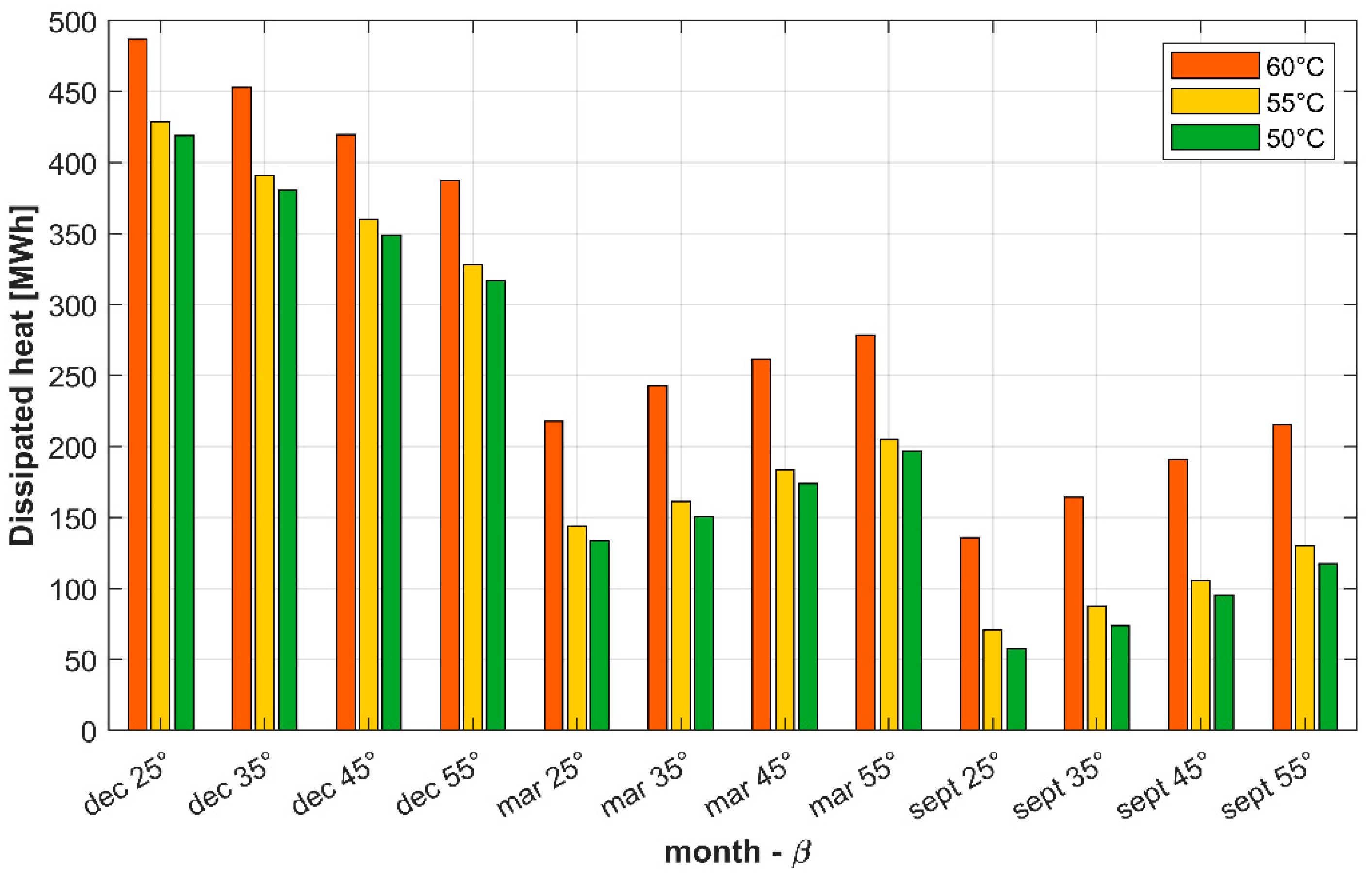
The annual dissipated heat (Figure 3) increased with TBT at the same β and design month, but this was significatively higher in the case of TBT = 60 °C compared to the other two cases. As shown later, at TBT = 60 °C $f_u$ was markedly lower, therefore less heat was consumed by the MED. The storage reached more frequently its maximum capacity and a greater amount of heat from the solar field had to be dissipated. The highest values of the annual dissipated heat for a given value of TBT were reached with December as the design month and the lowest with September. In fact, the design month of December led to an oversized solar field for the summer months. The annual dissipated heat had a different trend as a function of β for each design month. With December as the design month, the annual dissipated heat decreased with increasing β. Instead, with March and September as design months, it increased with β. For all the three values of TBTs, the minimum dissipated heat was reached with September as the design month and β = 25°. This was the case with the lowest $N_{coll}$ in the solar field.

Figure 4 shows the number of MED stop in the whole year. The number of plant on/off increased with TBT, but it was significatively higher in the case of TBT = 60 °C in comparison with the cases of TBT = 55 °C and 50 °C. The minimum number of plant on/off was obtained with the lowest TBT. In fact, a lower TBT increased the amount of heat in the storage that could be use by the MED. With the same storage volume and, consequently, with the same mass of hot water, a TBT of 50 °C allowed for the use the heat until the hot water in the storage reached a temperature of TBT + 15 °C = 65 °C (the hot water inlet temperature in the first effect). The highest number of plant on/off was obtained with September and the lowest with December as the design months at fixed β and TBT. With December as the design month, β had no influence on the number of MED stops independently of the value of TBT. With March and September as the design months, the number of plant on/off decreased with β. The minimum number of plant on/off was obtained, except with December as the design month, for the highest β (=55°). In fact, β = 55° was the optimal β in December, which was the month with the highest number of stops. The number of plant on/off almost did not depend on β when December was the design month. Indeed, the design of the solar field for December and for the each β ensured the limitation of plant on/off during winter, which is the most critical period of the year.

The annual utilization factor (Figure 5) increased with decreasing TBTs at the same β and design month. For TBT = 60 °C $f_u$ was markedly lower than the other two values of TBT in accordance with previous observations. At given β and TBT, the highest $f_u$ was obtained with December as the design month and the lowest with September as the design month. This can be explained because December as the design month led to a higher number of collectors while with September the solar field was undersized for the winter months. With December as the design month, β had almost no influence on $f_u$, independently of the value of TBT: The solar plant was sized for the worst condition (December) and for the given β. In the case of lower β, the higher $N_{coll}$ compensated for the lower collected energy per solar panel. With March and September as the design months, $f_u$ increased with β. In fact, higher values of β increased the solar energy collected in December, which was the month with the lowest solar irradiance; furthermore, with higher values of β, the number of collectors was higher; consequently, the MED operation hours increased in number.

3.2. Economic Analysis

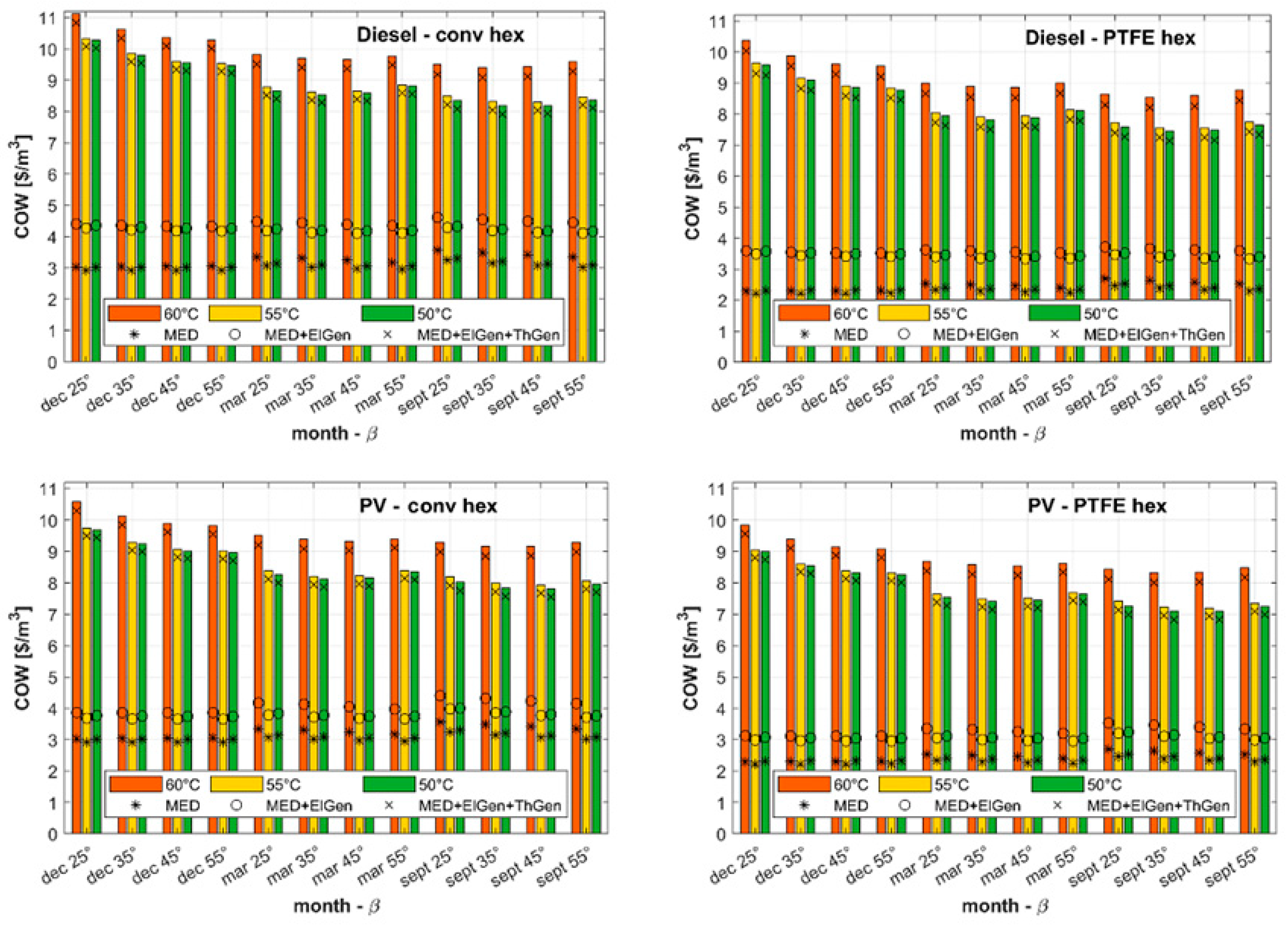
Figure 6 shows the COW for different values of TBT, design month, and β. The contributions of the MED unit, the electrical generation (diesel generator or PV system), and the solar field (ThGen) to the total cost are also shown. The difference between the COW and these three contributions was the storage cost contribution to the total COW.

It can be noticed that the COW increased with increasing TBT. At higher TBTs, the heat transfer areas of MED evaporators were smaller, leading to lower MED capital cost. However, this was not sufficient to compensate the effect of a lower $f_u$ and of a consequent lower desalted water production. The result was a higher component of the COW related to the MED plant (indicated with ‘*‘). Furthermore, the cost of the solar plant per cubic meter of desalted water (ThGen) was greater because of the greater number of collectors and of the lower water production (lower $f_u$).

The COW with the diesel generator (Figure 6) was higher than the COW in the case with the PV plant. In fact, despite the lower purchase and installation cost of the diesel generator with respect to the PV plant, the cost of fuel ensuring the continuous operation of water pumps led to an increase of the COW.

PTFE exchangers showed COWs lower by about 0.7–0.85 $\$/{\mathrm{m}}^3$ than conventional ones, corresponding to a reduction of 6.6–9.5% of the COW with conventional exchangers for the various simulated cases.

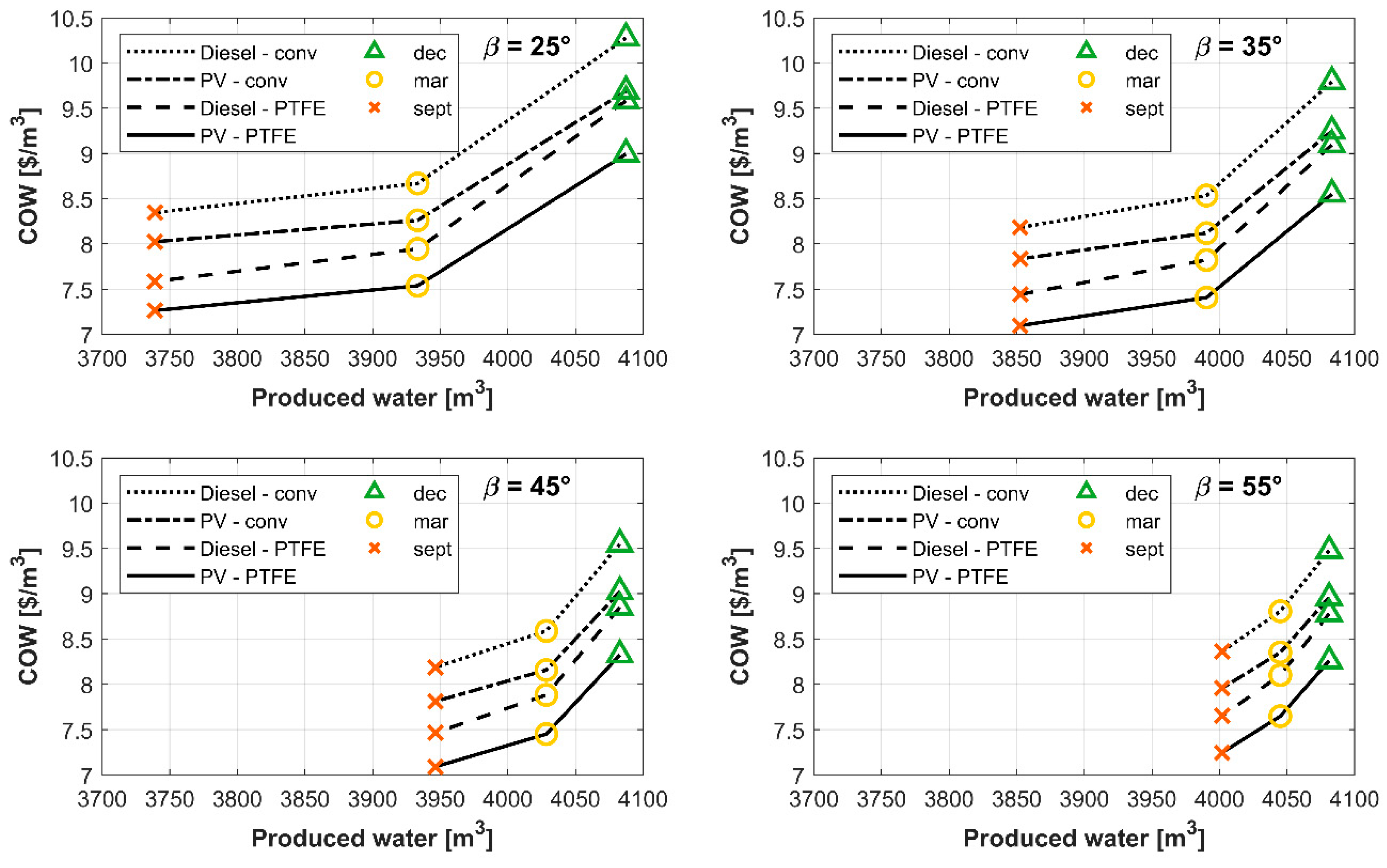
Figure 7 summarizes the results, reporting the obtained specific cost of water as a function of annual water production for different plant configurations, including the type of electric generation and material for the MED heat exchangers, for each value of β. For the sake of clarity, only the cases with TBT = 50 °C—the TBT showing the best results both in terms of the amount of produced water and of COW—are presented.

It is clear that some configurations are better than others, both in terms of COW and of yearly produced water. The maximum yearly produced water (about 4080 ${\mathrm{m}}^3$) was reached with December as the design month and it resulted almost independent of β. However, the choice of the highest value of β (55°) was preferable since it allowed for the lowest COW (8.26 $\$/{\mathrm{m}}^3$) among the cases with the maximum water production.

The lowest values for COW were reached with PTFE heat exchangers and the PV field for the electrical generation. The lowest COWs were obtained with September as the design month and with intermediate values of β (β = 35° and β = 45°) independently of the heat exchanger material and of the electrical generation system. The minimum COW of 7.09 $\$/{\mathrm{m}}^3$ was obtained with September as the design month and β = 45°, and gave a yearly water production of 3947${\mathrm{m}}^3$.

By using the TOPSIS method (Technique for Order Preference by Similarity to an Ideal Solution) with equal weights for the produced water and the COW, the recommended solution, shown in Figure 8, is that with September as the design month and β = 55°. This solution allowed for a lower number of collectors in comparison with configurations with other design months, but also a high utilization factor (greater than 95%).

4. Conclusions

The choice of the lowest TBT (50 °C) for the MED has been shown to be convenient not only in thermodynamic but also in economic terms, by lowering the COW. Indeed, the lowest TBT led to a high utilization factor for the MED.

PTFE heat exchangers allowed for the reduction of the COW by 6.6–9.5% for the various simulated cases in comparison with conventional exchangers.

The lowest COW was obtained with September as the design month, and with a tilt angle of 45°. The highest water production in the whole year was reached with December as the design month. Intermediate solutions to these two cases represent a compromise between having the lowest COW and producing the maximum amount of desalted water, and their choice can be made on the basis of the main purpose of the desalination plant.

The solar field is the component that has the major impact on COW (about 2/3) Therefore, the key point for the development of solar MED technology is the reduction of solar collector costs.