1. Introduction
Every year, many kilometers of underground cables and wires are installed around the world. In the last century, water, gas, electricity, sewerage, telephone, and internet wires have become widely available goods not only to residents of large urban agglomerations, but also to residents of small towns and villages. The development of material engineering, computerization, automation, and possibilities of equipment miniaturization enables the modernization old and development new technologies of pipelines construction, inspection, and renovation. Nowadays, underground installations are increasingly built using trenchless technologies as an alternative to traditional methods, i.e., open excavations [
1].
Using trenchless technologies, many problems are avoided, such as:
Technical (a need to overcome hills and close access roads);
Formal and legal (licenses and permits);
Economic (costs of renting large areas, compensations fees, penalties for environmental damage).
The use of trenchless technologies makes it possible to accelerate investment execution compared to traditional excavation methods. The increased durability of underground pipelines (less sensitivity to changes in atmospheric conditions than in case of surface pipelines) also supports the advisability of using drilling techniques in the construction of underground piping.
Some trenchless technologies, such as horizontal jacking, microtunneling, and Horizontal Directional Drilling (HDD), have been used in industrial practice for over 50 years. New technological solutions have also appeared on the market (direct pipe, reverse circulation, push hole-opening) and the existing ones have been modernized (HDD-intersect drilling) [
2,
3,
4].
One of the most commonly used technologies for constructing underground pipelines is HDD (in classic version or as intersect drilling) [
4].
Figure 1 presents the percentage comparison of primary Horizontal Directional Drilling markets.
The article focuses on two concepts of HDD trajectory design: The classic one, which is a combination of straight and curvilinear sections, and a chain curve trajectory-catenary. An attempt was made to create a methodology of calculations using optimization methods, taking into account theoretical issues and engineering design practice. The article develops the subject of HDD trajectory design presented in detail by the authors in their previous article [
6].
2. Concepts of Horizontal Directional Drilling Trajectory Design
The combination of straight and curvilinear sections [
6,
7] is one of the most commonly used concepts for designing HDD trajectories. The simplest variant of this method is to create a trajectory with one curvilinear section and a constant radius. Other variants are a combination of different numbers of straight and curvilinear sections. The practical experience shows that the optimum solution (from the technical, technological, organizational, and economic point of view) is a trajectory consisting of alternating straight and curvilinear sections (see
Figure 2a).
The second concept for designing HDD trajectories is associated with the natural deflection of the casing described by a chain curve (see
Figure 2b).
The chain curve trajectory (catenary) has many advantages, such as easier insertion of a pipeline into a wellbore and longer pipeline life cycle due to natural stress distribution along the length. Unfortunately, this type of well path trajectory is difficult to perform in real conditions because the angle of deviation from the horizontal plane is variable. Standard deflecting drilling tools do not allow continuous change of the deviation angle [
6].
At the AGH University of Science and Technology in Krakow at the Drilling and Geoengineering Department, Faculty Drilling Oil and Gas, algorithms enabling to design both types of the above-mentioned Horizontal Directional Drilling trajectories have been created. They were described in detail in the monograph [
8] and in the articles [
6,
9].
3. Methodology for Determining Fit of the Trajectory Being a Combination of Straight and Curvilinear Sections to a Catenary Trajectory
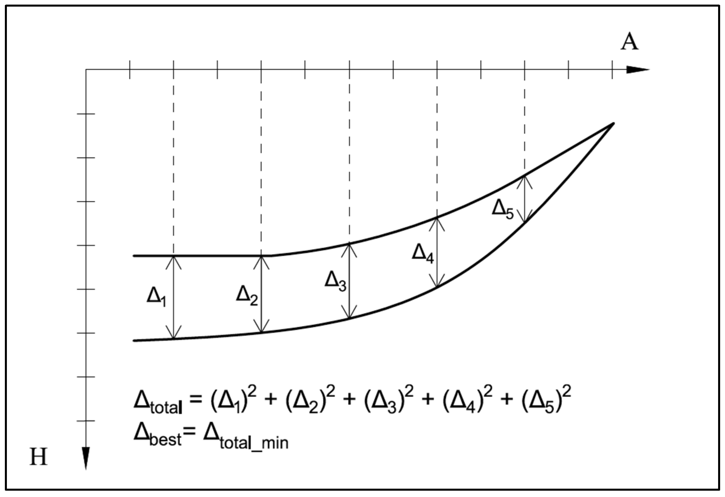
In the proposed methodology, a trajectory was designed as a chain curve, and then a sectional trajectory consisting of five sections was adapted to its shape. In order to find a sectional trajectory with the most similar shape to the catenary trajectory, it was necessary to define a function determining a similarity measure. In the article, the method of least squares known from statistical analysis was used [
10].
The best fit in the least-squares sense minimizes the sum of squares (the difference between sectional trajectory y
i values, and the catenary trajectory
value). A simplified concept is presented in
Figure 3.
Figure 4 shows the reference catenary trajectory and five classic five-section trajectories designed to visualize the problem (geometrical parameters of the five-section trajectory are presented later in the article). For the presented trajectories, the sum of squares (SOS) between the catenary trajectory and the five-section trajectory was calculated with a step of 1m. The results are presented in
Table 1.
The trajectories projection chart and calculated sums of squares (SOS) were presented above to show that a manual attempt to fit the trajectory is not a simple task. Based on
Figure 4 and the results in
Table 1, it can be seen that the proposed five-section trajectories differ significantly from the catenary trajectory. In this case, mathematical optimization needs to be done to calculate and search for sums of squares indicating the best fit (least squares).
4. Trajectory Parameters and Their Value Ranges Resulting from Technological Limitations and Assumed Goals
In order to obtain a five-section trajectory with a shape similar to the catenary trajectory, the sum of squares of trajectories should be minimized. To achieve that, it is necessary to find appropriate values of the equation parameters-optimize the five-section trajectory relative to the catenary trajectory.
During the optimization process, at the beginning, it is necessary to define ranges for the values of the trajectory equation parameters. The permissible values may result from technological limitations such an entry and exit angle (determined by the capabilities of a drilling device and a casing technology), bending radii (limited by strength of casing or drilled rock layers), and so on. One of the restrictions may be a distance between the entry and exit points.
Parameters that can be used to calculate five-section trajectories:
A–Horizontal displacement of the end point relative to the start point;
H–Vertical displacement of the end point relative to the start point;
L1–Length of the first section;
L3–Length of the third section;
ε1–Angle of deviation from the horizontal plane of the first section;
ε3–Angle of deviation from the horizontal plane of the third section;
ε5–Angle of deviation from the horizontal plane of the fifth section;
R2–Radius of curvature of the second section;
R4–Radius of curvature of the fourth section.
The geometrical dependencies for the five-section trajectory are presented in
Figure 5.
The end point displacements relative to the start point are constant horizontally (A) and vertically (H). This is due to the selected entry and exit points and their location, which must be the same for both trajectories.
An additional design constraint may be determinant of the first straight L1 section length in such a way as to enable the drilling tool to reach stable soils in which the angle of deviation can be changed. In another variant, the length of the third rectilinear section L3 can be a constraint, where it is necessary to allow drilling under a terrain obstacle (river, mountain, highway), under which accurate measurements of the position of a drilling tool are difficult or impossible to perform.
Another constant parameter is the angle of deviation of the third section of the trajectory from the horizontal plane (ε3). The value of this parameter is 0°. The third section is most often horizontal, which enables easier passage under an obstacle.
Entry (ε
1) and exit (ε
5) angles range between 6° and 15°. This limitation is related to the capabilities of drilling equipment and the casing pullback process. For strength reasons, it is assumed that their values should decrease as the casing diameter increases. For the same reasons, it is also recommended that the entry angle have a higher value than the exit angle [
11]. The latest bibliography gave even higher acceptable values of deviation angles: 8°–30° [
12]. The authors of [
13] stated that from the point of view of pipeline installation the ideal entry angle is 12° and the exit angle is 10°. In the article, values between 6°–16° were used for calculations.
The value of radii of curvature R
2 and R
4 depend on the diameter and type of casing. The larger the diameter, the larger the minimum radius. According to DCA [
10], the radius of curvature was determined from the formula:
Table 2 shows sample calculations of minimum bending radius using Equation (4).
Equations (2)–(4) are empirical, and the influence of the wall thickness on the bending stiffness of the pipe is neglected. Pipe stiffness increases along with the wall thickness, which makes bending more difficult. This tendency may result in higher soil reaction pressure exceeding, which may lead to breakdowns and drilling problems such as stuck pipe. These aspects were included in the below equation for the minimum bending radius [
14], adding the variables C (variable dependent on the type of soil) and t (wall thickness).
Table 3 shows sample calculations of minimum bending radius using Equation (5).
In the optimization calculations (presented later in the article), a radius range of 1500–3000 m was adopted for the casing with a diameter of 1 m.
5. Five-Section Trajectory Optimization
The process of searching for a five-section trajectory, the most similar to a catenary trajectory, was carried out using two methodologies: Searching the entire solution space and using the genetic algorithm.
5.1. Trajectory Optimization by Searching the Entire Solution Space
The simplest method for determining a five-section trajectory similar to the catenary trajectory is to calculate the parameters of a sectional trajectory and the sum of squares for all possible variants. Then, it is necessary to find input parameters for which the sum of squares is the smallest.
Figure 6 presents the simplified algorithm of the proposed methodology.
An algorithm for the variant with parameters (L1, R2, R4, ε1, ε5):
Determining the input data: Constants (A, H, Npoz), ranges of variables for which the optimization will be performed (L1min, L1max, Rmin, Rmax, εmin, εmax), and calculation steps for the optimized parameters (L1step, Rstep, εstep).
Calculation of spatial coordinates X, Y, and the alpha angle of the catenary trajectory.
Calculation of spatial coordinates X, Y, and the alpha angle of the five-section trajectory for each possible variant of L1, R2, R4, ε1, ε5 in nested iterations. At each calculation step, a sum of squares should be calculated for the corresponding points of the five-section and the catenary trajectory.
Finding the minimum value from the calculated sums of squares and the corresponding values: L1, R2, R4, ε1, and ε5.
Determining characteristic points of the trajectory being a combination of straight and curvilinear sections for the values determined in Item 4.
Advantages and disadvantages of the above methodology:
The optimization algorithm for the variant with parameters (L3, R2, R4, ε1, ε5) is analogous. (L3, L3min, L3max, L3step) should be used instead (L1, L1min, L1max, L1step).
5.2. Trajectory Optimization Using a Genetic Algorithm
The genetic algorithm is a method for solving optimization problems which belongs to evolutionary computation inspired by biology evolution. The idea of genetic algorithms is based on Darwin’s theory of evolution. In most cases, Nature applies two fundamental principles. First, if genetic processing results in offspring with above-average parameters, it usually survives longer and has a better chance of creating children with better traits than the average individual. Second, offspring with parameters below average will usually not survive—they will be eliminated from the population. Genetic algorithms can be used in cases where standard optimization methods are not applicable, for example, a given function is discontinuous, stochastic, nondifferentiable, or nonlinear [
15,
16].
Genetic algorithms are associated with terms such as population, an individual, generation, mutation, crossover, and the fitness function. A solution space is searched not by one point, but evenly by many points (individuals). This means that we can treat each individual as a representative of a problem solution at a given moment. These elements of genetic algorithms have been described in the literature [
15,
17].
An important and unique element of each genetic algorithm is the fitness function. It enables us to assess a degree of adaptation of an individual in the population. A better fit is a higher score, or a better chance of survival. It is closely connected with the problem being solved. For the analyzed case related to trajectories, the fitness function can be defined as:
where the Sum Of Squares( ) is determined from Equation (1).
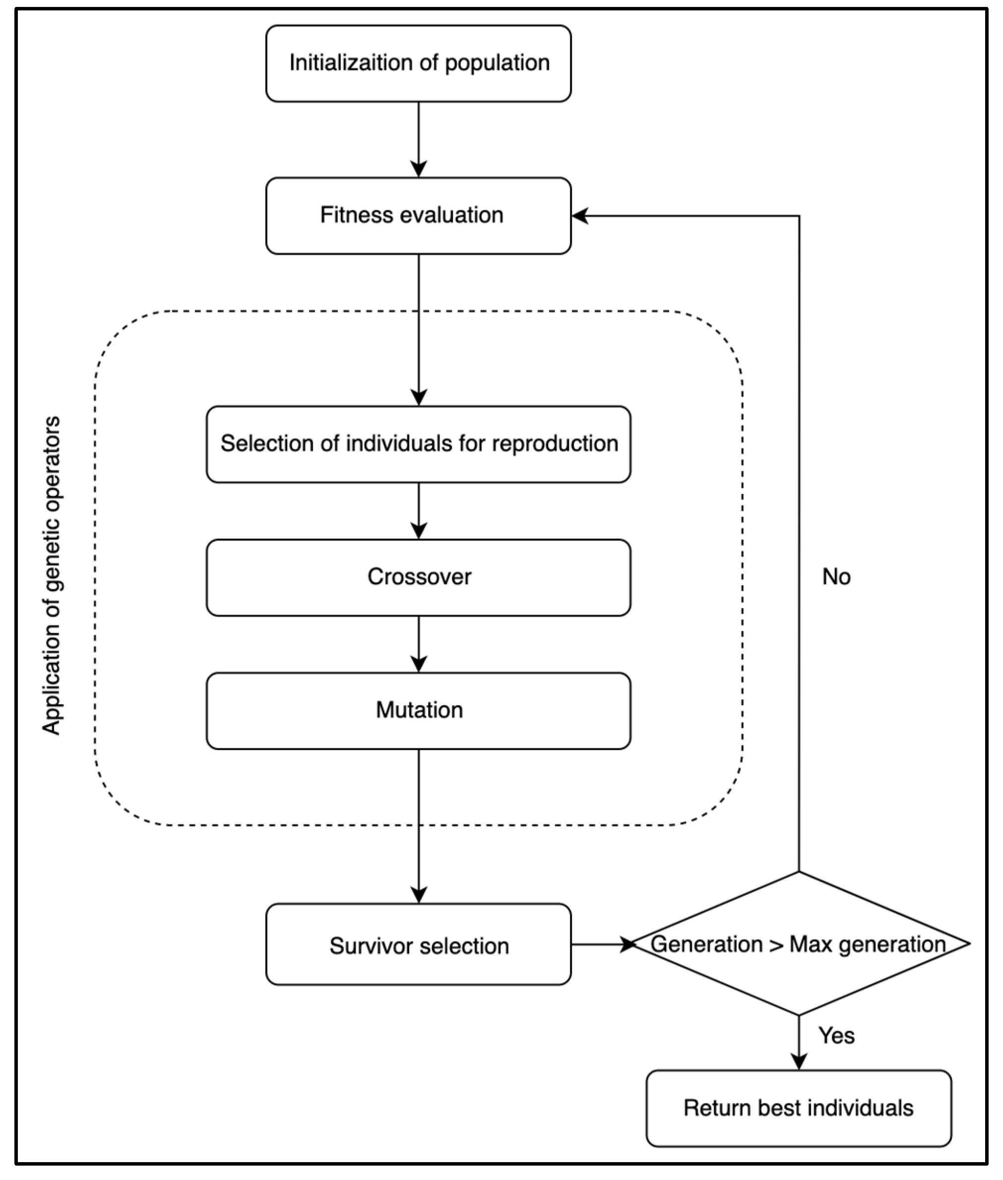
The value of the fitness function is within the range (0,1). The smaller the sum of squares, the greater the value of the fitness function. The genetic algorithm optimizes the parameters so that the value of the fitness function approaches 1. A general scheme of genetic algorithm is presented in
Figure 7.
6. Comparative Analysis of Calculation Methods
In order to compare the presented methods, a number of numerical simulations was performed for the variant of optimized parameters: L1, R2, R4, ε1, ε5. Their value ranges are presented below.
The catenary reference trajectory:
Horizontal displacement of the end point relative to the start point: A = 1000 m.
Vertical displacement of the end point relative to the start point: H = −15 m.
Casing weight: q = 800 N/m.
Drilling rig pulling force: Npoz = 250,000 kgf.
Azimuth: B = 0° (horizontal drilling performed northward).
Five-section trajectories:
Radius of the first curve section: (second section of the trajectory): R2 ∈ [1500,3000] m.
Radius of the second curve section: (fourth section of the trajectory): R4 ∈ [1500,3000] m.
Length of the first rectilinear section (first section of the trajectory): L1 ∈ [1,301] m.
Entry angle: ε1 ∈ [−16,−6]°.
Exit angle: ε5 ∈ [6,16]°.
Table 4 presents the results of numerical simulations of searching for a five-section trajectory similar to the catenary trajectory by means of searching the entire solution space. In subsequent series, the change of parameter values in iterations was smaller, thanks to which it was possible to find more suited trajectories (SOS decreases).
Table 5 and
Figure 8 show the results of a simulation using a genetic algorithm with the fitness function from Equation (6). For this method, for simplifying data entry, no parameters calculation steps are required, and their value can be any rational number. The parameter that enables control of the accuracy of calculations is the maximum amount of generation or the minimum permissible value of the fitness function. SOS decreases as the fitness function increases.
The above tables (see
Table 4 and
Table 5) present the results of calculation times and SOS values for two optimization methods. On their basis, both methods can be compared. Searching the entire solution space took 1066 ms to find a catenary-like trajectory with SOS = 845.62. For comparison, by means of the genetic algorithm, a similar trajectory was found in 112.4 ms, giving the value of SOS = 604.26. In subsequent series, the difference in computation time becomes apparent as can be seen in the comparison in
Table 6.
The above comparison is very general, but it simply shows a significant difference in computation times. The method using the genetic algorithm was much faster, and with an increase in the computation accuracy (reducing the SOS), the calculation time ratio increased in favor of the genetic algorithm.
7. An Example of the Application of the Presented Computation Methods in Engineering Design
Based on the analysis of computation times, it was demonstrated that the genetic algorithm method is much faster. The difference can be particularly observed when the expected accuracy of fitting increases. For the given parameters, while expecting to achieve high computational accuracy, performing search of the entire solution space is too time consuming. The speed of calculation using the genetic algorithm is very high. It should be noted here that the results obtained using the genetic algorithm are rational numbers. In the engineering approach, such parameter accuracy may be too high. For instance, measuring and drilling devices usually have an accuracy of 0.5 degrees to determine the inclination angle. For this reason, the authors propose to use the optimization method with a genetic algorithm at the initial design stage. It will save time if the designer performs many comparative simulations. Once the narrowed down parameter ranges of the optimized trajectory are established, the method of searching the entire solution space should be used. It will enable the designer to obtain engineering calculation steps with reasonable computation time. The calculation schema may be presented in the following way:
- (A)
Determination of the catenary (reference) trajectory.
- (B)
Calculation of initial values of trajectory parameters using a genetic algorithm.
- (C)
Determination of narrowed down parameters ranges and calculation steps reasonable from engineering point of view.
- (D)
The use of the method of searching the entire solution space with the determined narrowed down parameters ranges and calculation steps.
Application Example
In order to show the practical application of the proposed methodology, calculations of the HDD trajectory under a terrain obstacle were made. The obstacle makes it impossible to conduct telemetry measurements. For this reason, it was decided that the section under the obstacle would be rectilinear and horizontal with the minimum length of 100 m. At the same time, it was desirable to obtain a trajectory shape as close to the catenary trajectory as possible.
The assumption regarding the minimum length of the third section of the trajectory means that a calculation variant with optimization of L3, R2, R4, ε1, ε5 parameters should be used. Additional assumptions are presented in particular calculation steps.
(A) Determination of the catenary (reference) trajectory.
In the first step, the designer has to establish the main assumptions for calculating the reference trajectory. Assumptions for the analyzed case:
Horizontal displacement of the end point relative to the start point: A = 1000 m.
Vertical displacement of the end point relative to the start point: H = −15 m.
Casing weight: q = 800 N/m.
Drilling rig pulling force: Npoz = 250,000 kgf.
Azimuth: B = 0° (horizontal drilling performed northward).
Results:
The catenary reference trajectory was determined on the basis of the algorithm presented in the article [
6]. The results of the calculations are summarized in
Table 7.
(B) Calculation of initial values of trajectory parameters using a genetic algorithm.
In this step, the designer should use the optimization with a genetic algorithm:
Radius of the first curve section (second section of the trajectory): R2 ∈ [1500,3000] m.
Radius of the second curve section (fourth section of the trajectory): R4 ∈ [1500,3000] m.
Length of the second rectilinear section (third section of the trajectory): L3 ∈ [100,400] m.
Entry angle: ε1 ∈ [−16,−6]°.
Exit angle: ε
5 ∈ [
6,
16]°.
Table 8 presents initial values of five-section trajectory parameters calculated using a genetic algorithm.
Parameters determining the fit and the computation time:
(C) Determination of narrowed down parameters ranges and calculation steps reasonable from engineering point of view.
Based on the results from the optimization with the genetic algorithm, the parameter ranges can be narrowed down. Calculation steps can be set with reasonable accuracy from the engineering point of view:
Radius of the first curve section (second section of the trajectory): R2 ∈ [2400,2500] m, step 10 m.
Radius of the second curve section (fourth section of the trajectory): R4 ∈ [2300,2400] m, step 10 m.
Length of the second rectilinear section (third section of the trajectory): L3 ∈ [100,110] m, step 1 m.
Entry angle: ε1 ∈ [−9,−8]°, step 0.5°.
Exit angle: ε5 ∈ [7,8]°, step 0.5°.
(D) The use of the method of searching the entire solution space with the determined narrowed down parameters ranges and calculation steps.
Due to the narrowed down parameter ranges and engineering calculation steps, the computation time using the method of searching the entire solution space is short. This is possible to achieve due to significant reduction in the number of iterations (in calculations performed based on the algorithm presented in
Figure 6).
Table 9,
Table 10 and
Table 11 present characteristic and geometric values of the trajectories obtained during the optimization process.
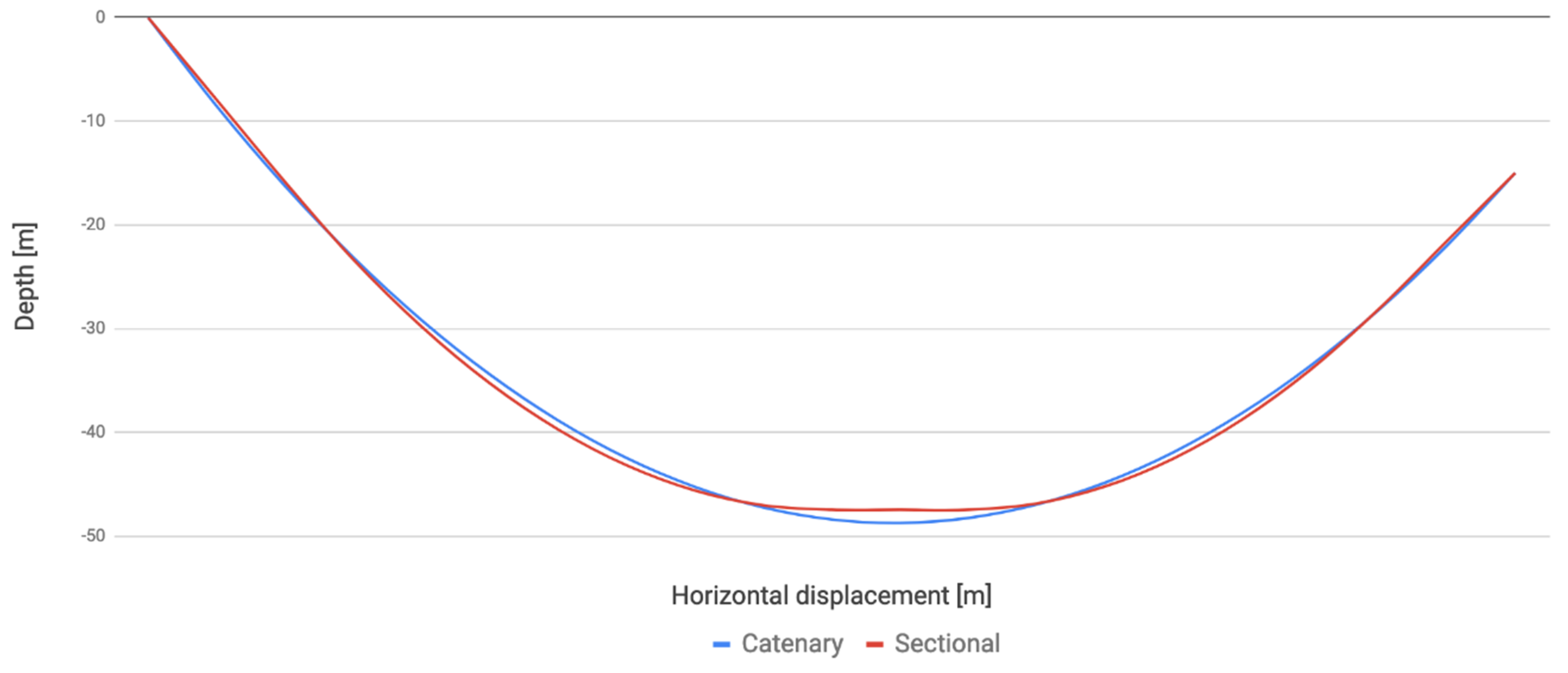
Figure 9 shows the comparison between the catenary reference trajectory and the trajectory obtained from optimization.
Parameters determining the fit and the computation time:
8. Conclusions
The effectiveness of the HDD technology is highly determined by its properly designed trajectory. Drilling failures and complications, which often accompany the application of HDD, result from a wrong selection of the well path trajectory in relation to the existing geological and drilling conditions.
In the design process, two concepts of HDD trajectory designing should be considered: Classic five-section, being a combination of straight and curvilinear sections, and a chain curve trajectory (catenary). Taking into account the advantages and disadvantages of the catenary trajectory relative to the five-section trajectory, an original solution was proposed, which was to make a five-section trajectory with a shape as similar to a catenary trajectory as possible.
Optimizing of the five-section trajectory relative to the catenary trajectory requires complex numerical calculations. The optimization methods presented in this article, namely searching the entire solution space and the genetic algorithm, can be used to perform such calculations, as has been proven in the article.
The genetic algorithm makes it possible to perform optimization much faster than the method of searching the entire solution space for comparable SOS values. The differences in computation times are so large that the use of the searching the entire solution space method is almost impossible from the design point of view.
Given the engineering design process and the need to adjust the results to technological and technical capabilities, it is reasonable to combine both methods to improve calculations. The computational example presents the benefits of conducting initial calculations using the genetic algorithm and then searching the narrowed down space of solutions with the accuracy that is technologically feasible to achieve.
Author Contributions
Conceptualization, R.W., P.Ł., and G.O.; Methodology, R.W., P.Ł., and G.O.; Software, P.Ł., and G.O.; Validation, R.W., P.Ł., and G.O.; Formal Analysis, R.W., P.Ł., and G.O.; Investigation, R.W., P.Ł., and G.O.; Resources, R.W., P.Ł., and G.O.; Data Curation, R.W., P.Ł., and G.O.; Writing–Original Draft Preparation, R.W., P.Ł., and G.O.; Writing–Review & Editing, R.W., P.Ł., and G.O.; Visualization, R.W., P.Ł., and G.O.; Supervision, R.W.; Project Administration, R.W. All authors have read and agreed to the published version of the manuscript.
Funding
This research received no external funding.
Conflicts of Interest
The author declares no conflict of interest.
Nomenclature
| Aj—projection of the jth section on a horizontal plane | [m] |
| β—azimuth | [°] |
| D—pipe diameter | [mm] |
| DLSj—dogleg severity | [°/m] |
| εj—angle of deviation from horizontal plane at the jth characteristic point | [°] |
| Hj—projection of the jth section on a vertical plane | [m] |
| Lj—length of jth section | [m] |
| Npoz—drilling rig pulling force | [N] |
| q—casing weight per meter | [N/m] |
| SOS—sum of squares | [-] |
| Ri—radius of curvature of jth section | [m] |
References
- Stein, D.; Mölers, K.; Bielecki, R. Microtunelling; Verlag für Architektur und technische Wissenschaften: Berlin, Germany, 1989. [Google Scholar]
- Australian Drilling Industry Training Committee Limited. The Drilling Manual; CRC Press: Boca Raton, FL, USA, 2015; ISBN 978-0-429-15054-8. [Google Scholar]
- Wiśniowski, R.; Druzgała, A.; Formela, M.; Toczek, P. Intersect Drilling Method; SGEM: Vienna, Austria, 2018; Volume 18. [Google Scholar]
- Yan, X.; Ariaratnam, S.T.; Dong, S.; Zeng, C. Horizontal directional drilling: State-of-the-art review of theory and applications. Tunn. Undergr. Space Technol. 2018, 72, 162–173. [Google Scholar] [CrossRef]
- Underground Construction UC Exclusive: 21st Annual Horizontal Directional Drilling Survey. Available online: https://ucononline.com/magazine/2019/june-2019-vol74-no-6/features/uc-exclusive-21st-annual-horizontal-directional-drilling-survey (accessed on 2 May 2020).
- Wiśniowski, R.; Skrzypaszek, K.; Łopata, P.; Orłowicz, G. The Catenary Method as an Alternative to the Horizontal Directional Drilling Trajectory Design in 2D Space. Energies 2020, 13, 1112. [Google Scholar] [CrossRef]
- Willoughby, D. Horizontal Directional Drilling: Utility and Pipeline Applications; McGraw-Hill: New York, NY, USA, 2005; ISBN 978-0-07-145473-5. [Google Scholar]
- Wiśniowski, R. Selected Aspects of Directional Wells Construction Design with the Use of Numeric Methods; AGH: Kraków, Poland, 2002. [Google Scholar]
- Wiśniowski, R.; Stryczek, S. Projektowanie trajektorii horyzontalnego przewiertu sterowanego. (ang. Horizontal Directional Drilling trajectory design). Wiert. Nafta Gaz 2007, 24, 929–941. [Google Scholar]
- AGH Univeristy of Science and Technology Analiza regresji (ang. Regression analysis). Available online: http://home.agh.edu.pl/~kca/stat/WYK%A3ADY_pdf/WYK%A3AD%20%2011.pdf (accessed on 3 May 2020).
- Drilling Contractors Association (DCA-Europe) DCA Technical Guidelines. Horizontal Directional Drilling. Information and Recommendations for the Planning, Construction and Documentation of HDD Projects; Drilling Contractors Association: Houston, TX, USA, 2001. [Google Scholar]
- Wen, J. A Novel and High-Efficiency Reaming Assembly for Underground Pipelines Pulling Back Laying in Horizontal Directional Drilling. DEStech Trans. Environ. Energy Earth Sci. 2019. [Google Scholar] [CrossRef]
- American Society of Civil Engineers. Pipeline Crossings; ASCE Publications: Reston, VA, USA, 1996; ISBN 978-0-7844-7409-9. [Google Scholar]
- da Silva, D.M.L.; Rodrigues, M.V.; Venås, A.; de Medeiros, A.R. Methodology for Definition of Bending Radius and Pullback Force in HDD Operation. In Proceedings of the Rio Pipeline Conference Proceedings, Rio de Janeiro, Brazil, 22–24 September 2009. [Google Scholar]
- Flasiński, M. Introduction to Artificial Intelligence; Springer International Publishing: New York, NY, USA, 2016; ISBN 978-3-319-40020-4. [Google Scholar]
- Genetic Algorithm Terminology—MATLAB & Simulink. Available online: https://www.mathworks.com/help/gads/some-genetic-algorithm-terminology.html (accessed on 14 May 2020).
- Kramer, O. Studies in Computational Intelligence. In Genetic Algorithm Essentials; Springer International Publishing: New York, NY, USA, 2017; ISBN 978-3-319-52155-8. [Google Scholar]
© 2020 by the authors. Licensee MDPI, Basel, Switzerland. This article is an open access article distributed under the terms and conditions of the Creative Commons Attribution (CC BY) license (http://creativecommons.org/licenses/by/4.0/).


