A Mixed Integer Linear Programming Model for the Optimization of Steel Waste Gases in Cogeneration: A Combined Coke Oven and Converter Gas Case Study

Abstract

Off-gas is one of the by-products of the steelmaking process. Its potential energy can be transformed into heat and electricity by means of cogeneration. A case study using a coke oven and Linz–Donawitz converter gas is presented. This work addresses the gas allocation problem for a cogeneration system producing steam and electricity. In the studied facility, located in northern Spain, the annual production of the plant requires 95,000 MWh of electrical energy and 525,000 MWh of thermal energy. The installed electrical and thermal power is 20.4 MW and 81 MW, respectively. A mixed integer linear programming model is built to optimize gas allocation, thus maximizing its benefits. This model is applied to a 24-h scenario with real data from the plant, where gas allocation decision-making was performed by the plant operators. Application of the model generated profit in a scenario where there were losses, increasing benefits by 16.9%. A sensitivity analysis is also performed. The proposed model is useful not only from the perspective of daily plant operation but also as a tool to simulate different design scenarios, such as the capacity of gasholders.

1. Introduction

Despite the improvements made by the steel industry, reducing greenhouse gas emissions is still a global challenge. The energy consumed in the entire steel production process represents a very significant percentage of economic and environmental costs. Using the basic oxygen furnace route, approximately 89% of the energy comes from coal, 7% from electricity, 3% from natural gas, and 1% from other gases [1]. According to the same report, when using an electric arc furnace route, the energy input from coal accounts for 11%, that from electricity accounts for 50%, that from natural gas is 38%, and 1% comes from other sources (data calculated from Worldsteel LCI database, 2018). Therefore, the efficient use of energy is very important for reducing total operational costs.

Steel waste gases, which are produced in a continuous and inherent way, can be transformed into other forms of energy, such as electricity and steam. These gases, which are considered byproducts, are increasingly used for this purpose, and there are considerable worldwide efforts to study their effective utilization. A comprehensive review can be found in [2,3].

Because steel waste gases have the advantage of being a secondary fuel while avoiding greenhouse emissions at the same time, different consumers within factories compete for these gases. Under this context, optimization methods are useful to determine the best distribution of available resources.

In iron and steel works, there is usually a misbalance between the amount of by-product gases produced and those consumed. Gasholders and other buffers are used to solve this fluctuation. The allocation of surplus gases among gasholders, boilers, engines, and other consumers is studied using scheduling and optimization problems to maximize economical profits and minimize emissions.

The main objective of this work is to obtain a model that serves as a decision-making aid system to optimize the operation of cogeneration plants that use various fuels, particularly coke ovens and converter gases complemented with natural gas. The model considers operational, economic, and environmental constraints. The facility is located inside a steelmaking plant in northern Spain, which is a complex and singular facility that produces electricity and steam from waste steel gases. This plant combines simple cycle cogeneration technology with engines specially adapted for operation with converter gases and steam generated in boilers that mainly consume gas from coke oven batteries (but also complemented with converter and natural gases). In total, 707 MWh of electric power can be produced per million m³ of converter gas and 11,800 tonnes of vapor per million m³ of coke oven gas. The converter process is a Linz–Donawitz (LD) type, in which blowing oxygen through molten pig iron lowers the carbon content of the alloy, transforming it into low-carbon steel.

In 2017, Zhao et al. [4] published a review on the optimal scheduling of by-product gases in the steelmaking industry that will help us introduce the novelty of our present work. The authors noted two primary challenges in by-product steel gas scheduling. First, in previous studies, the efficiency of the boilers was set as a constant despite being unrealistic in real practice. The main points impeding efficiency are surplus gas fluctuation and the requirement that the operational load must follow the time-of-use power price. The authors suggested that the non-linearity of boiler efficiency should be considered. The modeling presented here prioritizes boilers that work at full load and thus avoid working at partial loads, for which the equipment shows much lower performance. Secondly, the authors stated that planning using real time prices is a new and interesting area to be investigated to achieve a better peak-valley of the power load. The present work facilitates the simulation of scenarios considering the real daily prices of the electricity market. The proposed model is useful for decision-making in cogeneration plants. In Spain, the price of electricity is known 24 h in advance. This constitutes the time window for planning the use of gases since a predetermined service level must be maintained for steam production. The inflow of gases can be forecasted according to the plant production program. This model allows the optimal control of gasholders, storing off-gas during the valley price period and releasing more during the peak price period, and overcoming all the technical constrains, such us gasholders capacity. Other important limitations depend on the operational ranges of the designs for each piece of equipment and the plant in general. This model may also be valuable for simulating different gasholder capacities, thus helping the strategic design decision-making process.

In this paper, a mixed integer linear programming (MILP) model is developed. The goal is to maximize the overall benefit, thereby optimizing off-gas distribution in the cogeneration plant. This model assists the decision-making process by providing the optimal solution for any situation that may arise. A one-day scenario using real data gathered from operations under normal conditions is analyzed to illustrate how this model works.

This paper is organized as follows. First, the steel gas cogeneration process (SGCP) is introduced. Then, the method is described, and the mathematical formulation is presented. Next, the use case scenario is described. To illustrate the usefulness of the system, a real use case with a 24 h time window is used. The results provided by the model are compared to the actual operational data. Finally, the main conclusions and future research are provided.

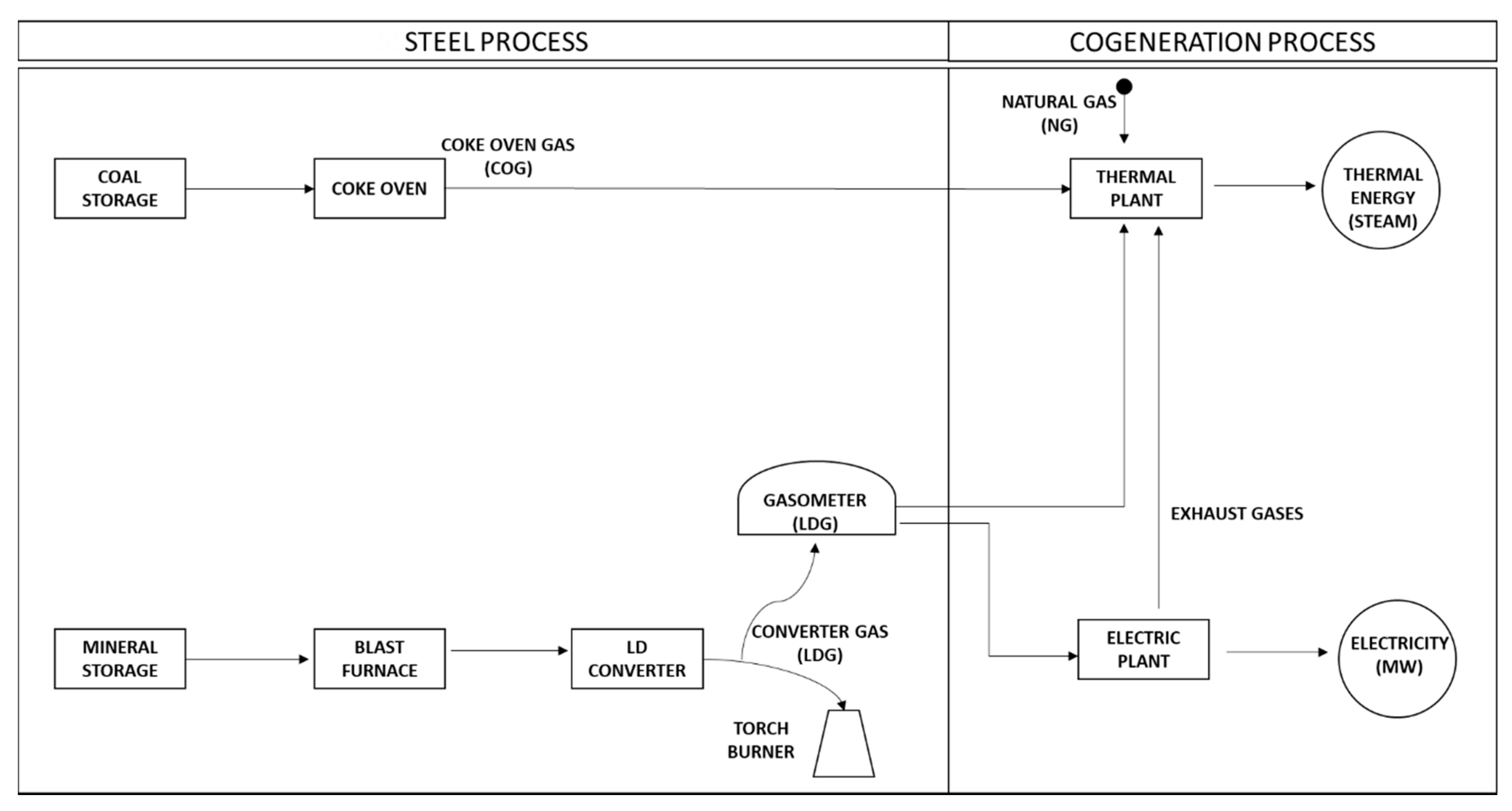
2. Process Description

The fuels of the studied facility are coke oven gas (COG) fuel and Linz–Donawitz converter gas (LDG) fuel. Coke gas is a by-product of industrial coke production from pit coal. It is generated by the high-temperature dry distillation of coking coals in the absence of oxygen. This gas consists mainly of hydrogen, methane, and a small percentage of carbon monoxide, carbon, and nitrogen. It constitutes a high-value fuel for effective power generation due to its high calorific power. Converter gas is created from pig iron during the steel production process. The LD process is the most common production method used to generate raw steel. By means of this process, the pig iron is refined with oxygen, lowering the carbon proportion and providing enough process heat to maintain the steel liquid.

Table 1. Main characteristics of coke oven gas and Linz–Donawitz converter gas.

COG	LDG
Pyrolisys	Blown oxygen
Coke batteries	LD converter
>50% H2, CH4	70% CO, CO2
4000 kcal/Nm3	2100 kcal/Nm3
SH2, NH3 and heavy oils	Quite clean
Difficult energy utilisation	Highly toxic

summarizes the main characteristics of each gas. The calorific power of COG is almost double that of LDG, but the latter is a cleaner gas. The actual composition of both gases for this plant is detailed in

Table 2. Average composition of coke oven gas and Linz–Donawitz converter gas. Source [5].

	Units	COG	LDG
CO	%	5.44	68.21
H2	%	58.14	1.05
CH4	%	24.36	0.02
C2H6	%	0.61	-
N2	%	5.57	12.95
O2	%	0.45	0.6
CO2	%	1.38	13.42
H2O (VAP)	%	2.21	3.75
Density	Kg/Nm3	0.434	1.3242
SGCP	Kcal/Nm3	4512	2104
PCI	Kcal/Nm3	3988	2099

.

In an SGCP, these by-product gases are valorized by special engines to produce electricity in the electric plant and by boilers in the thermal plant to produce steam. Figure 1 provides a schematic view of the production process and subsequent use of the gases. The electric plant works only with LDG; meanwhile, the thermal plant runs mainly with COG but also with LDG or natural gas (NG) when the production of steelmaking gases is insufficient to supply the thermal energy required by the steel factory. The energy contained in the engine jacket water is also used to heat the boiler feed water up to 95 °C, and the energy of the engine exhaust gases is expelled at 500 °C for the production of recovery steam. This helps minimize thermal losses and reduces both the consumption of other resources and the emissions into the environment, as described in [6].

The steel factory requires approximately 90 tonnes/h of steam. The thermal energy is supplied by three conventional boilers, type FDU-3527, with a multifuel burner (coke gas, converter gas, or natural gas) with a steam production of 35 tonnes/h and a nominal power of 27 MW, as well as a recovery boiler, type GV-201, with a steam production of 20 tonnes/h and a nominal power of 11 MW. The equipment includes an economizer, vaporizer, and superheater, as well as a chimney for the evacuation of gases with a bypass in the economizer. This process is depicted in Figure 2.

The plant includes 12 groups of gas engines that provide a total net electric power of 20,400 kW. The exhausts gas is recovered through a heat recovery unit for the generation of steam. The unit is designed as compact modular groups integrated with an engine, an alternator, and auxiliary systems for fuel, cooling, lubrication, and boot. Gas engines, designed to operate with converter gas, are a four-stroke type that provide turbocharging and cooling of the air–gas mixture and the electronically regulated combustion of the lean mixture. This process is depicted in Figure 3.

The electricity produced is commercialized in the daily electrical market. The steam is entirely consumed by the steelmaking plant. The temperature of the superheated steam is 300 °C, which is controlled through an attemperator system with an outlet pressure of 1.9 MPa.

In this kind of environment, there is an imbalance between the produced and consumed gas. Production is irregular and depends on very complex factors, such as planning production orders, mineral stocking, scheduled maintenance, breakdowns, incidents, and many other issues. The gasholders are a key element that balance the process. Since the storage capacity of the gasometers is limited, the correct planning and management of waste gases is crucial. This decision-making process usually relies on the empirical knowledge of the plant managers. Therefore, it is convenient to apply optimization techniques.

This case study is different compared to existing works. Conventional cogeneration plants are usually formed by the boiler and turbine assembly working in series. However, this study combines two related but independent processes: the boilers always produce steam, but the engines can be stopped without generating electricity. This aspect is very important because, in addition to electrical energy, the use of the thermal energy contained in the engines has special relevance for the operation of the thermal plant. Because of all this, the optimal management of steel gases has a very important impact on plant performance.

3. Method

The problem was modelled as a constraint satisfaction problem. This kind of problem can be defined by a set of variables, the domains for each of the variables, and the constraints on the values that the variables might assume simultaneously [7]. Different families of optimization models are used to formulate and solve these kinds of problems. One of the most successful methods is MILP modelling.

MILP models are one of the most prominent tools for solving the optimization of by-product gas systems and achieving cost reduction. Akimoto et al. [8] were the first to use MILP to optimize the by-product gases in the iron and steel industry. A mathematical model was formulated by Kim et al. [9,10], whose objective was to minimize the total cost over multiple periods. Kim et al. [11] also achieved an optimal trade-off between conflicting objectives, such as reducing the number of burners on/off and reducing holder level changes, thereby minimizing fuel consumption costs.

Compared to previous works, Kong et al. [12] proposed a model that simultaneously optimizes the distribution of by-product gases in the by-product gas system, the cogeneration system, and the iron- and steelmaking system. Qi et al. [13] developed a model for the plant-wide optimization of by-product gases to reduce the total cost. In their study, the authors proposed a more precise and objective penalty weight as a constraint in the function. De Oliveira et al. [14] presented a model to solve the problem of by-product fuel distribution to maximize energy utilization and assign appropriate weights to the objective function penalties, resulting in an increase in the operational performance of the fuel distribution system. Song et al. [15] noted that the dynamic optimization of surplus gas distribution has a very important position in the management of gas systems and established a common model. Zeng et al. [16] incorporated a novel multi-period model for the optimal distribution of by-product gases as steam and power. Different by-product gases can be mixed to satisfy the minimum heating and energy requirements of production units. Moreover, the authors introduced key practical features of by-product gases, steam, and power generation and distribution. Orre et al. [17] evaluated methods for decreasing the total energy demand and CO₂ emissions in a system containing an integrated steel plant connected to a combined heat and power plant through optimized production operations for seasonal-dependent energy demands.

Pena et al. [18] carried out a sensitivity analysis of the objective function considering the penalties associated with the decision variables of the optimization problem to evaluate the price of fuel used in a thermoelectric plant with a high market value, which should replace the gases generated in the steelmaking process only when the reserves of stored gas are small. Later, the same authors [19] minimized the imbalance between the random dynamics of by-product fuel generation and consumption and maximized the energy efficiency under various uncertainties using adaptive time-series models. Considering the time-of-use electricity price, Zhao et al. [20] proposed a model to optimize the by-product gas used. This model was later extended by considering Pareto optimality and fuzzy sets to find the best solution for two conflicting objectives: achieving gasholder stability and reducing the electricity purchasing cost [21].

The model was implemented using IBM ILOG CPLEX Optimization Studio software (CPLEX) [22]. CPLEX is software developed by IBM to solve optimization problems. CPLEX is a comprehensive tool designed to facilitate building and solving integer programming problems, very large linear programming problems (using either primal or dual variants of the simplex method or the barrier interior point), convex and non-convex quadratic programming problems, and convex quadratically constrained problems (solved via second-order cone programming). This tool combines integrated and full-featured development and supports OPL (optimization programming language) and high-performance CPLEX and CP Optimizer solvers. CPLEX has been selected because it is one of the most powerful and extended software optimization packages that can be used freely for academic applications. The suite has been in continuous improvement since the first version developed by Robert Bixby in 1988 [23]. The version used for this work was CPLEX Studio 12.9.0. Using the studio, optimization problems can be modelled using OPL, an easy-to-use declarative language. OPL allows the model to be separated from the data in two different declarative files: model file and data file. It is easy to simulate different scenarios using this feature. The models are defined in terms of decision variables, the objective function and constraints. The model files may also include scripts for pre- or post-processing the data. OPL syntax is very close to the natural way that a mathematical constraints optimization problem is expressed. This package has also been selected because of this feature, so starting the implementation from the mathematical formulation is easy, and also to carry on the model to other optimization packages. As a benefit, our work is more easily replicable.

The steps performed for this modelling can be summarized as follows:

• First, the boundaries of the system are established, and the processes are identified. Reasonable simplifications are introduced to describe the system mathematically. This process is depicted in Section 2.
• Second, an optimization model is created. The objective functions and constraints are both presented (Section 4).
• Third, an appropriate optimization routine is applied. In this study, CPLEX is used to solve the MILP problem.
• Fourth, the model is validated using a scenario, and the results are analyzed.

4. Problem Formulation

4.1. Objective Function

The subobjectives of the multifuel cogeneration process are to maximize energy revenue sales (1), minimize fuel costs (2), and minimize CO₂ emission costs (3). All these objectives are considered independently to explain the influence and impact of each separately. Subsequently, they are grouped into an overall objective function (4) to maximize the profit of the process. The numbers in parentheses refer to the equations that describe each component. Equipment maintenance cost (5) is also considered but not included within the objective function, as justified in Section 4.6.

4.2. Revenue

Revenue from energy sales (R) consists of:

• Remuneration for the sale of electric energy (R_EE): this is obtained by multiplying the electric energy generated by the hourly price of the electric pool, given by P_POOL[t].
• Remuneration for the sale of thermal energy (R_TE): this is obtained from the product of steam produced compared to the price paid by the steel factory (in this case, a fixed price, given by P_TE).

$$R={\displaystyle \sum _{t=0}^{23}}\left(R_{EE}[t]+R_{TE}[t]\right)={\displaystyle \sum _{t=0.23}^{}}\left(P{R}_{EE}[t]\ast P_{POOL}[t]+P{R}_{TE}[t]\ast P_{TE}\right).$$

(1)

The analyzed temporal window (t) is 24 h. The electric power production (PR_EE) is calculated by multiplying the amount of LDG allocated for electric production by the heat value of LDG. The thermal value is calculated in a similar way while also considering the amount of each gas allocated (thermal production could be performed with any of the three gases).

4.3. Fuel Cost

This is the amount of gas consumed in the SGCP to produce electrical and thermal energy multiplied by its unit cost:

$$C_{FUELS}={\sum }_{t=0.23}\left(Q_{LDG}[t]\ast P_{LDG}+Q_{COG}[t]\ast P_{COG}+Q_{NG}[t]\ast P_{NG}\right).$$

(2)

The cost of the gas is fixed (not time-dependent) and is given by P_LDG (cost of LDG in €/Nm³), P_COG (cost of COG in €/Nm³) and P_NG (cost of GN in €/Nm³) in the equation. Q_LDG, Q_COG, and Q_NG are the cumulative amount of gas consumed per hour for each kind of fuel. Natural gas is consumed only for producing electricity and COG only for thermal energy, but LDG is consumed for both thermal and electrical power production. Thus, we must consider the amount allocated to each use: Q_LDG = Q_{LDG_EE} + Q_{LDG_TE}.

4.4. Emission Cost

This model considers CO₂ emissions. The cost is estimated using the conversion factor for each of the fuels recovered in the SGCP according to Equation (3):

$$C_{CO2}={\displaystyle \sum _{t=0.23}}\left(Q_{LDG}[t]\ast {\mu }_{LDG}+Q_{COG}[t]\ast {\mu }_{COG}+Q_{NG}[t]\ast {\mu }_{NG}\right)\ast P_{CO2}$$

(3)

where μ represents the emission factor of each type of gas, and P_CO2 is the cost per ton of CO₂ emissions.

4.5. Profit

The profit of the plant includes all of the above conditions:

$$Profit=R-C_{FUELS}-C_{CO2}$$

(4)

4.6. Manteinance

Maintenance cost (C_MTE) is derived from the number of stops of the equipment. For the burners, the unitary cost is represented by α, and for the engines β. The installation also has fixed maintenance costs, but these are not considered as they remain constant.

$$C_{MTE}=\alpha \ast \sum STOP{S}_{BURNERS}+\beta \ast \sum STOP{S}_{BOILERS}$$

(5)

Equation (5) is not included within the overall goal because the number of stops cannot be modelled with the linear programmer of OPL. Although at first glance it seems easy to compute, and it would be with a standard programming language, the OPL modelling language is limited to mathematical expressions within the context of linear programming. To calculate it, we would need to compare the fuel consumption of one hour with that of the previous one, to detect equipment starts, and accumulate the number of on/offs. However, this cannot be done either in the section of the code dedicated to working with decision variables or in the section where the restrictions are declared. We are doing this calculation using CPLEX scripts post-processing the results. Therefore, we calculate the cost that it has, but this cost is not considered in the optimization. This is a limitation of the model. However, the maintenance cost is negligible compared to the rest of the costs.

4.7. Constraints

The overall goal of this model is to maximize profits according to the following constraints.

4.7.1. Gas Availability

Natural gas and COG are available without limitations, but LDG is produced discontinuously depending on the melts of the steelworks and is captured and conducted to a gasholder, as depicted in Figure 1. Therefore, the first restriction refers to the fact that LDG consumption must not exceed the gasholder’s amount available at any time:

$${\displaystyle \sum _{i=0.t}}\left(Q_{LDG\_TE}[i]+Q_{LD{G}_{EE}}[i]\right)\le {\displaystyle \sum _{j=0.t}}{F}_{LDG}[i]+stoc{k}_{LDG}\forall tin[0.23]$$

(6)

where Q_{LDG_ET} and Q_{LDG_EE} are the amount of LDG allocated for electric and thermal power respectively, F_LDG is the flow of gas captured from steelmaking, and stock_LDG is the amount of surplus LDG stored by the gasholder in the previous period (at time t = 0).

4.7.2. Gasholder Constraints

As previously stated, gasholders play a key role in this process. In this case, the LDG gasholder that acts as a buffer for the gases captured from the conversion process is constrained by the maximum capacity (V_{LDG_MAX}) and the minimum capacity (V_{LDG_MIN}). The profit of the system is largely determined by the proper management of the capacity of this gasholder. Equation (7) and (8) model these constraints:

$$stoc{k}_{LDG}+{\displaystyle \sum _{i=0.t}}\left(F_{LDG}[i]-Q_{LDG}[i]\right)\ge V_{LDG\_MIN}\forall tin[0.23]$$

(7)

$$stoc{k}_{LDG}+{\displaystyle \sum _{i=0.t}}\left(F_{LDG}[i]-Q_{LDG}[i]\right)\le V_{LDG\_MAX}\forall tin[0.23]$$

(8)

4.7.3. Steam Demand Satisfaction Constraint

The steam generated from the boilers must meet the energy demands (D_TE) for each period, which are shown in Equation (9):

$$P{R}_{TE}[t]\ge D_{TE}[t]\forall tin[0.23]$$

(9)

The thermic production (PR_TE) is calculated according to the gas’s heat value described in Section 4.2 (revenue).

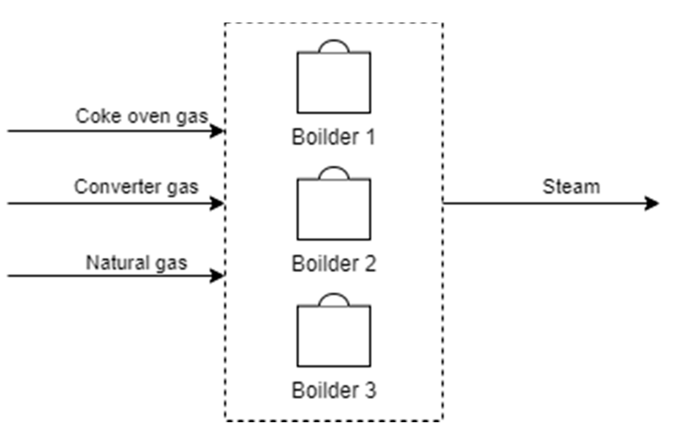
4.7.4. Boiler Constraints

Boilers have their operational ranges and cannot operate under their technical limits. They require a minimum gas flow threshold to be started, as modeled in Equation (10), (11), and (12):

$$Q_{LDG\_TE}[t]\ge LD{G}_{\underset{boiler}{\min }}\parallel Q_{LD{G}_{TE}}==0\forall tin[0.23]$$

(10)

$$Q_{COG}[t]\ge GO{C}_{\underset{boiler}{\min }}\parallel Q_{GOC}==0\forall tin[0.23]$$

(11)

$$Q_{NG}[t]\ge N{G}_{\underset{boiler}{\min }}\parallel Q_{NG}==0\forall tin[0.23]$$

(12)

These three equations are equivalent; the only difference is that Equation (10) considers that LDG may be consumed for thermal or electrical power, so the equation considers the flow to be thermally allocated. These equations can also be parameterized to distinguish different levels for each boiler (for example, in the case study, there are three boilers). However, the boilers that are used generally have the same technical characteristics.

A very important factor is the use of the “OR” operator (noted as “‖” in the equations). This is used in the sense that the CPLEX solver will assign 0 to that variable (the allocated gas) if the minimum threshold of the boiler is not reached. In this way, the boiler does not start if there is not a minimum gas flow.

In a similar way, the boilers cannot burn more fuel than the upper limit. This is modeled according to Equations (13–(15):

$$Q_{LDG\_TE}[t]\le LD{G}_{\max \_boiler}\forall tin[0.23]$$

(13)

$$Q_{COG}[t]\le GO{C}_{\max \_boiler}\forall tin[0.23]$$

(14)

$$Q_{NG}[t]\le N{G}_{\underset{}{\max \_\mathrm{boiler}}}\forall tin[0.23]$$

(15)

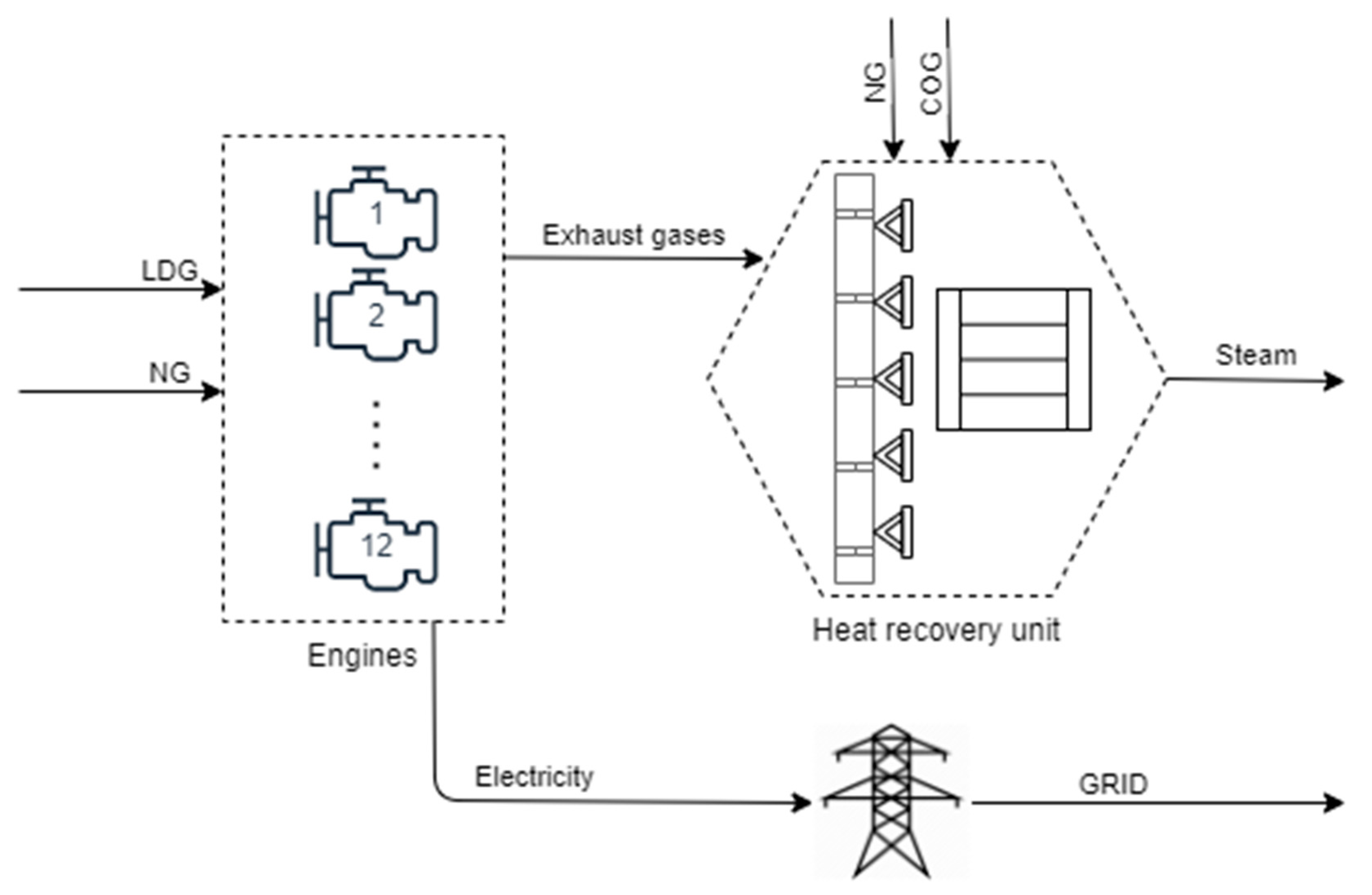
4.7.5. Engine Constraints

The engines for electric production are also subject to operational constraints. In this case, the number of equations is more significantly reduced because the engines can only operate with LDG.

$$Q_{LDG\_EE}[t]\ge LD{G}_{\min \_engine}\parallel Q_{LD{G}_{EE}}==0\forall tin[0.23]$$

(16)

$$Q_{LDG\_EE}[t]\le LD{G}_{\max \_engine}\forall tin[0.23]$$

(17)

The “OR” operator is used in Equation (16) as it is used in Equation (10) within the context of the CPLEX solver to avoid the engine from starting if the minimum gas threshold is not reached.

4.8. OPL Model

Appendix A includes part of the CPLEX OPL source code. The code starts with the data section. All the variables and data structures are declared within this section. It is necessary to consider that the data is loaded from a complementary .dat file, so the variables are initialized with those values. In this way, the same model can be used to easily simulate different scenarios. This file is not included, but the values of the variables can be easily derived from the description of the scenario in Section 5.

The second section includes the declarations of the decision variables. In that section, dvar is the OPL keyword used to declare decision variables. Some expressions can be used to write more complex expressions in a compact way. In this case, the subobjectives stated in Section 4.2, Section 4.3 and Section 4.4 are written using decision expressions. Finally, the objective must be stated. In this case, maximize the overall profit.

The third section contains the model constraints. Here, all the problem formulation described in Section 4.7 is coded. Finally, the model also includes scripts for post-processing the results and to perform additional calculations. This section has not been included in the Appendix A due to its length and because it is not of special interest.

5. Scenario Description

To begin, we detail the installation parameters that are relevant to the formulation of the problem.

Table 3. LDG gasholder capacity parameters.

Parameter	Capacity (Nm3)
Lower threshold	10,000
Normal	45,000
Upper limit	61,000

shows the capacity of the LDG gasholder. Once the upper limit is reached, the untapped LDG is directly burned by the torch.

The efficiency of each type of equipment is shown in

Table 4. Efficiencies of each type of equipment.

Equipment	Units	Start Year	Type	Nominal Power (MW)	Performance
Boilers	3	2004	FDU-3527	27	92%
Gas engine	12	2004	JMS 620 GS-S/NL	1.7	35.5%

. Frequently starting and stopping the equipment should be avoided, which can be enforced by penalties. The penalty for each engine stop was established as 10 € due to the mandatory maintenance costs for every 2000 engine starts. For each burner stop, 5 € was established to avoid the risk of unwanted unavailability. Finally, 70 € was determined for each boiler stop to reduce the work of partial loads on the boilers and the consequent loss of performance, according to Zhao et al. [20]. These penalties were established according to the plant operators’ experience.

Table 5. Consumption ranges of the boiler gases.

Gas	Range [min-max] (Nm3/h)
COG	[1200–4000]
LDG	[2000–10,000]
Natural Gas	[400–4000]

and

Table 6. Consumption ranges of the electric engines.

Gas	Range [min-max] (Nm3/h)
COG	-
LDG	[1100–2000]
Natural Gas	-

present the consumption ranges of the equipment for different gases. The electric engines are adapted to work only with LDG.

The heating values of fuel gases and the factor emissions are shown in

Table 7. Heating values of steel gas cogeneration.

Gas	Heating Values (MJ/m3)	Factor Emission (kG CO2/GJ)
COG	16.9	42.32
LDG	8.8	185.47
Natural Gas	36.1	55.83

. A penalty for CO₂ emissions must also be considered. For the computation, 5.96 €/t was the average value registered for the geographical area of the plant during the period of study (2014).

The revenue of steam production is fixed by contract and is shown in

Table 8. Revenue for steam production.

Gas	Revenue (€/t)
COG	3.6
LDG	3.6
Natural Gas	2.4

. The price paid is higher for steel gas due to the environmental benefits that it provides to the factory by avoiding torch combustion.

The planning period spans one day with real data from the operation in SGCP. The time step length of 1 h corresponds to the actual measuring period used in the process. The thermal energy required by the steel process must be supplied by the cogeneration plant in a continuous, safe, and reliable way. For electric energy, the objective is to maximize energy sales based on the hourly price of the electricity market. In Spain, this price is known the day before as a consequence of crossing the energy supply and demand curve forecasting. The electricity spot market defines the prices for every hour of the following day. For this reason, the correct management and optimization of gas flows is essential to ensure the fewest repercussions for the performance of the thermal plant.

The management of off-gas is currently done manually and based on the knowledge of the operators. The operating data were recorded for the plant over one year. The data differ in the amount of available steel gases, as well as the steam demands and electricity prices. Based on a study of these data, a scenario was selected; this scenario is considered representative of the different situations that may occur. The operation and performance of the current results are compared and evaluated against the results of the optimization model proposed in this work.

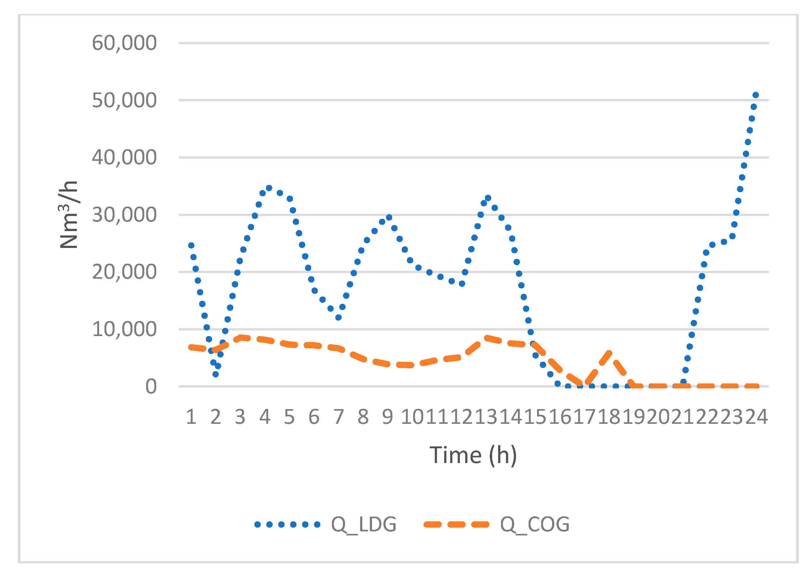
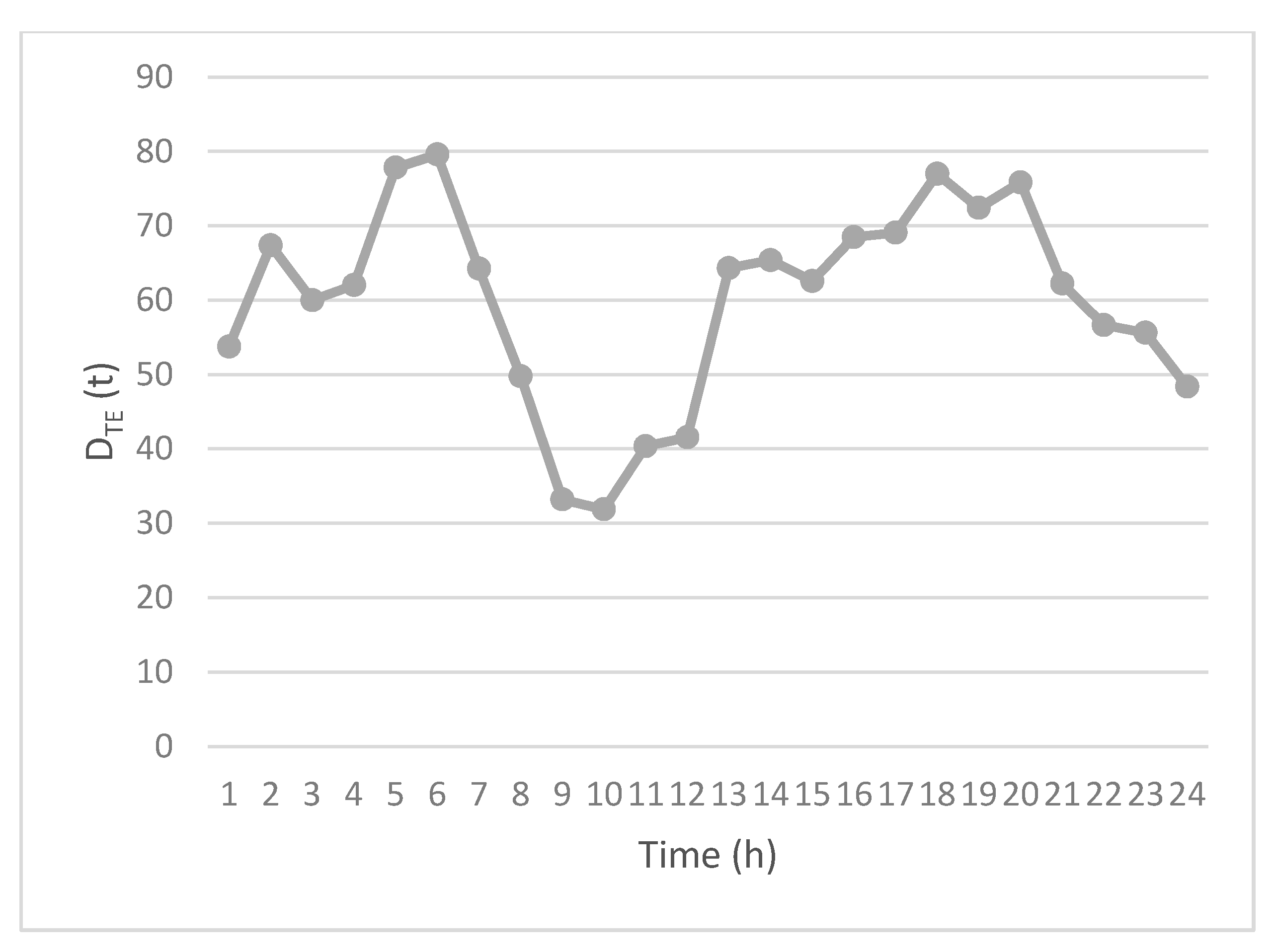
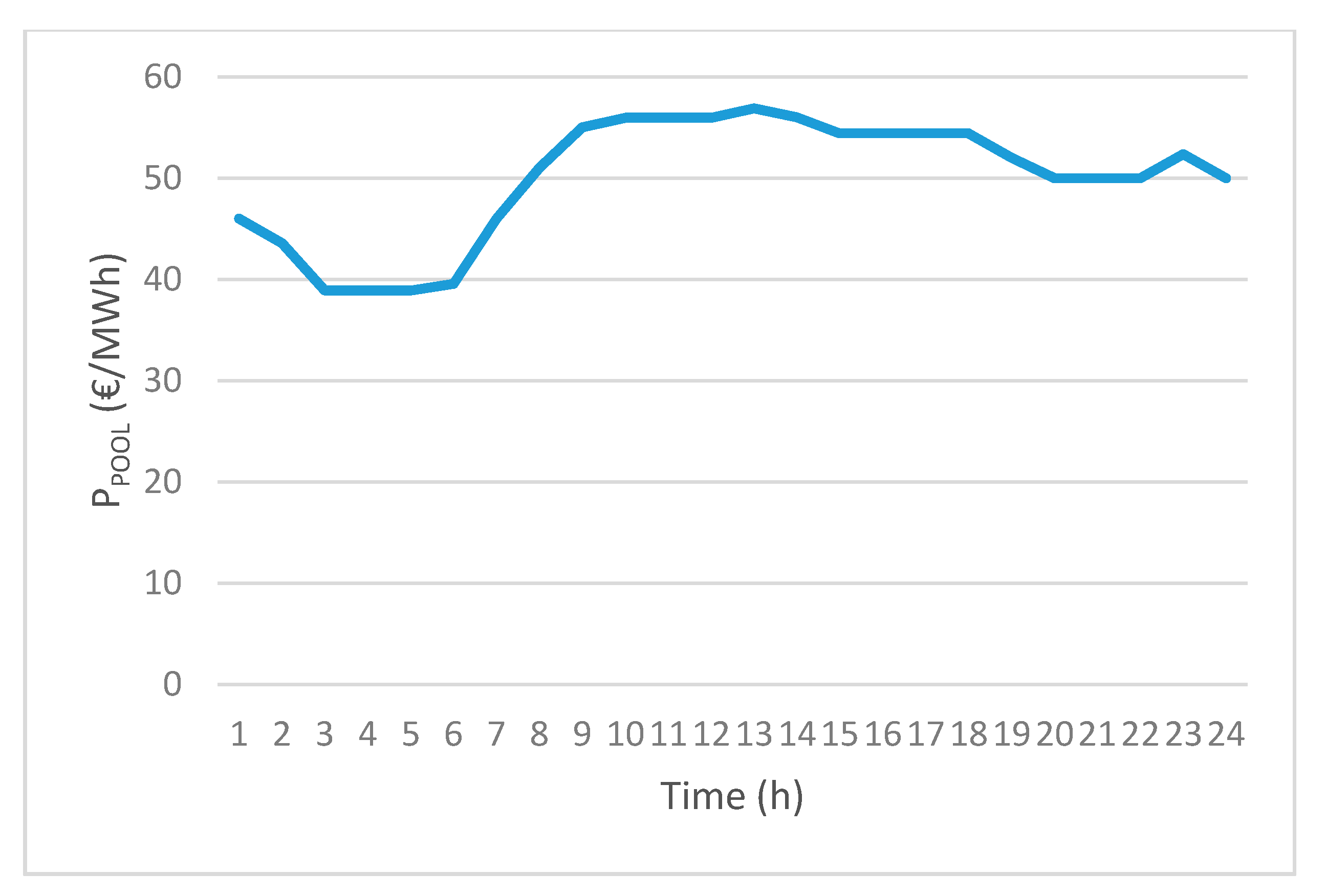
5.1. 24-h Reference Scenario Data

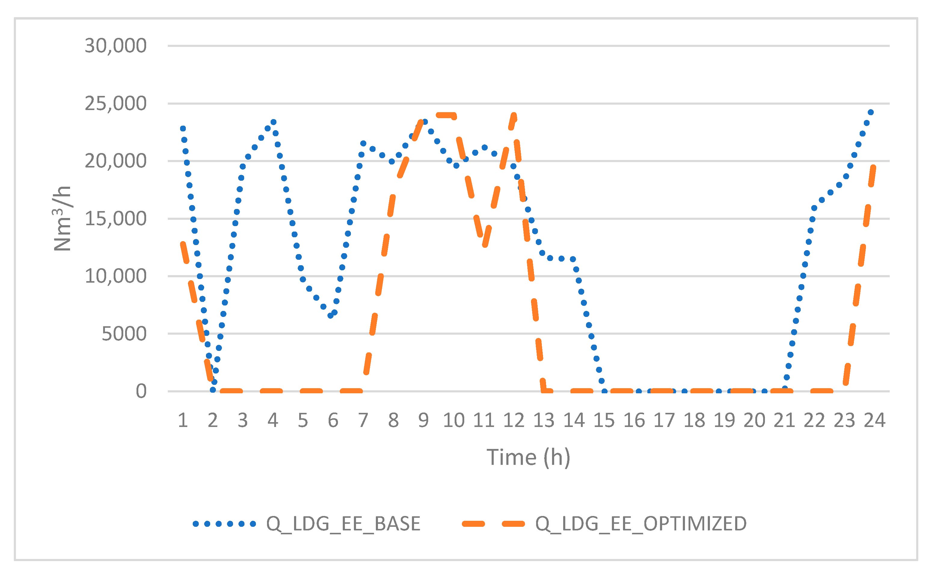
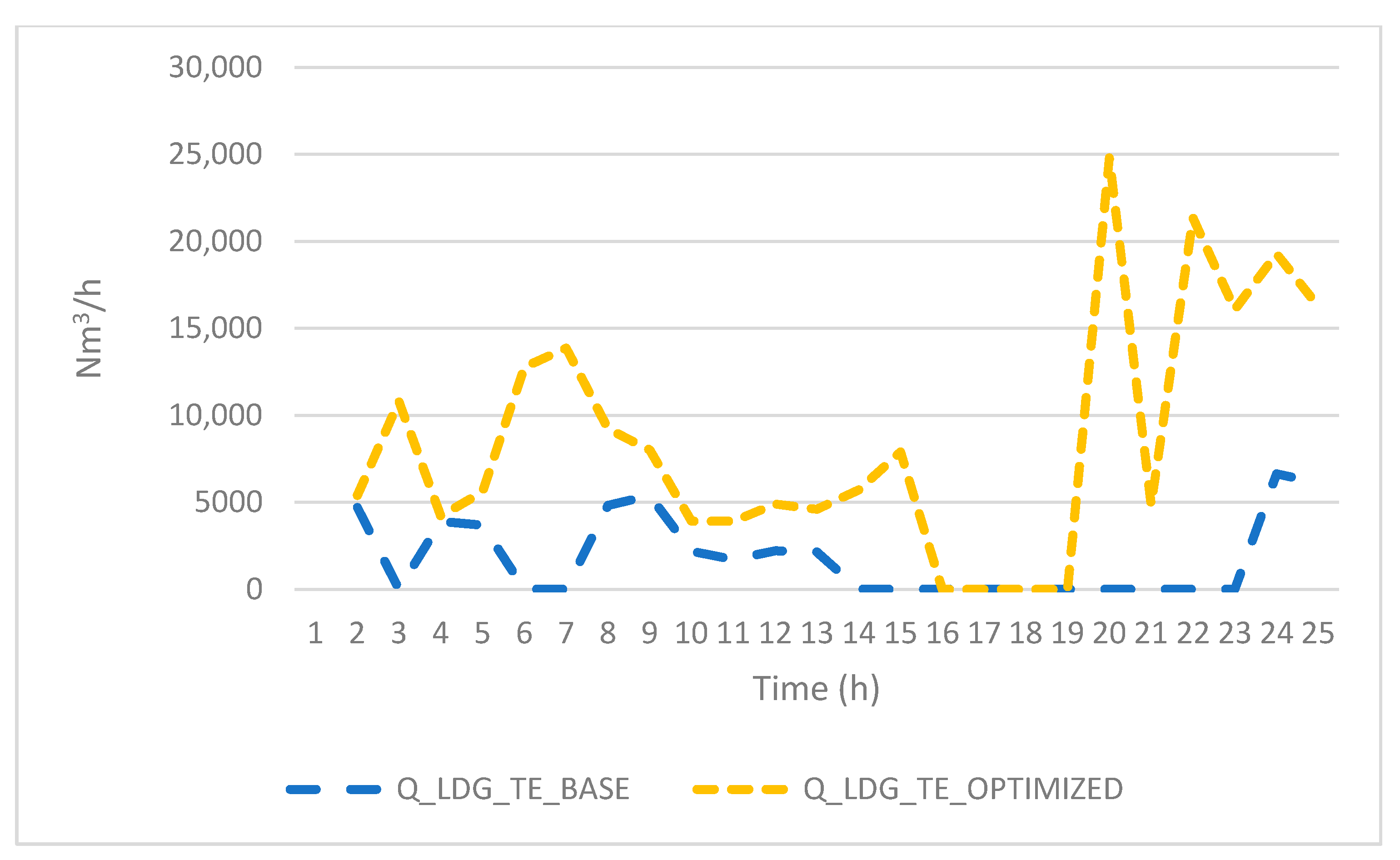
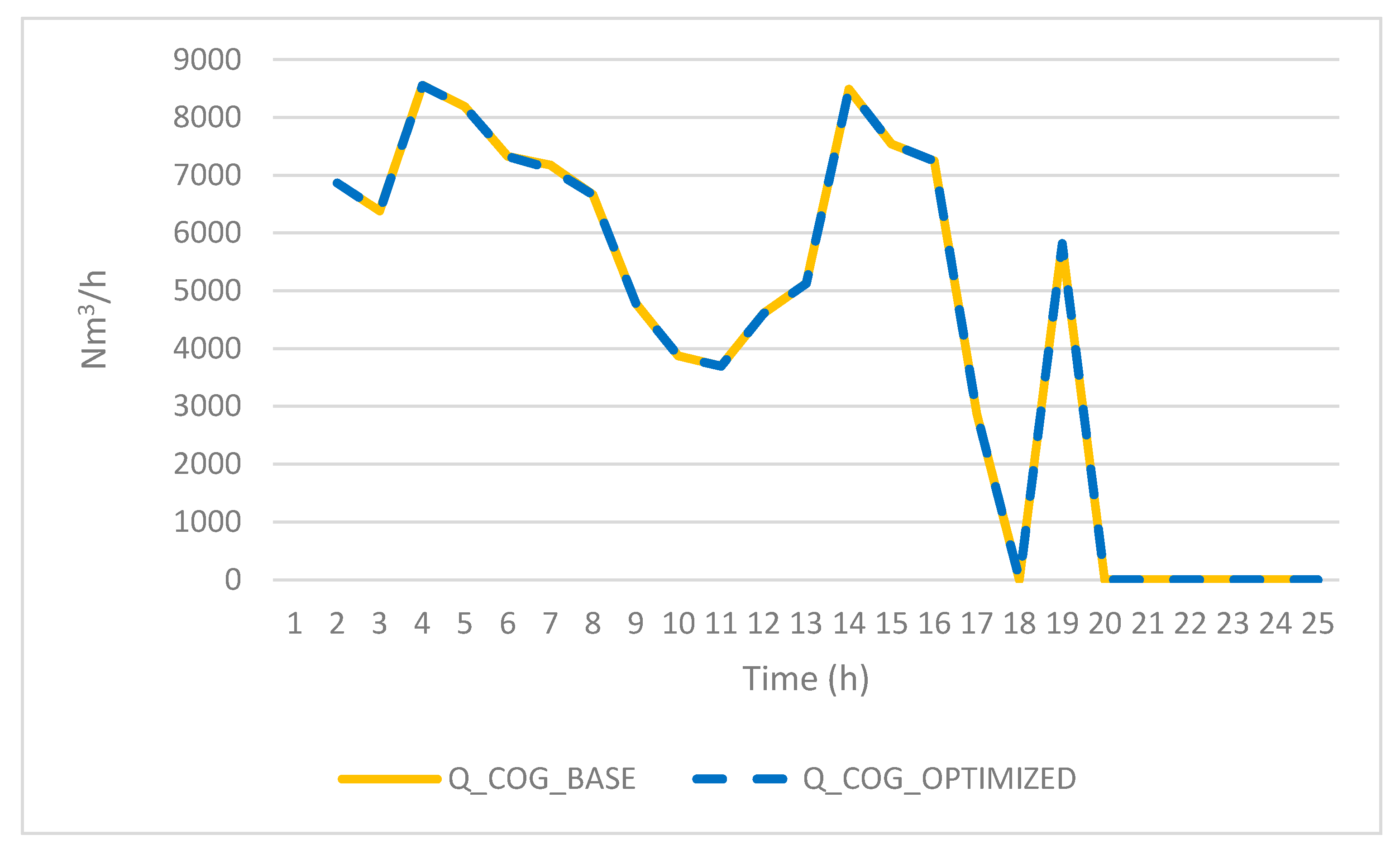
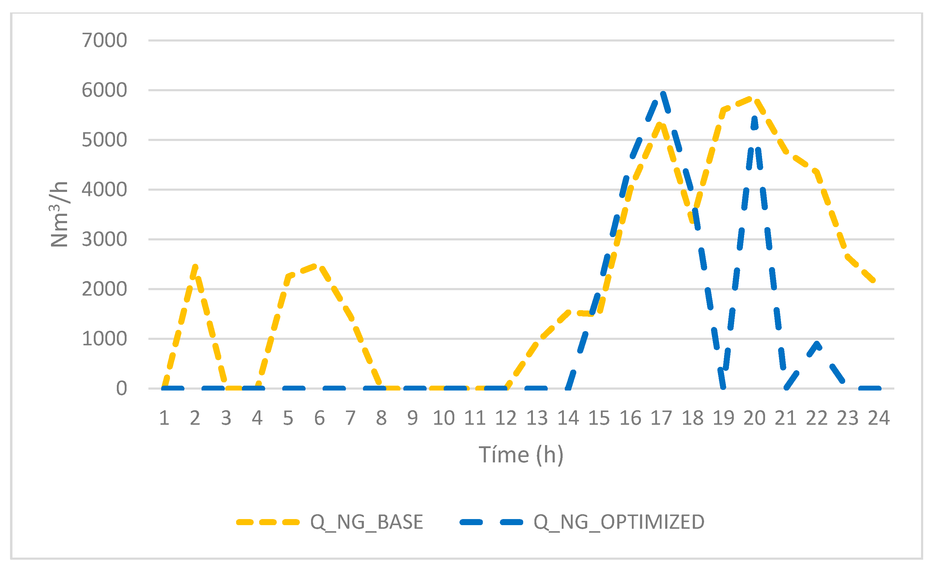
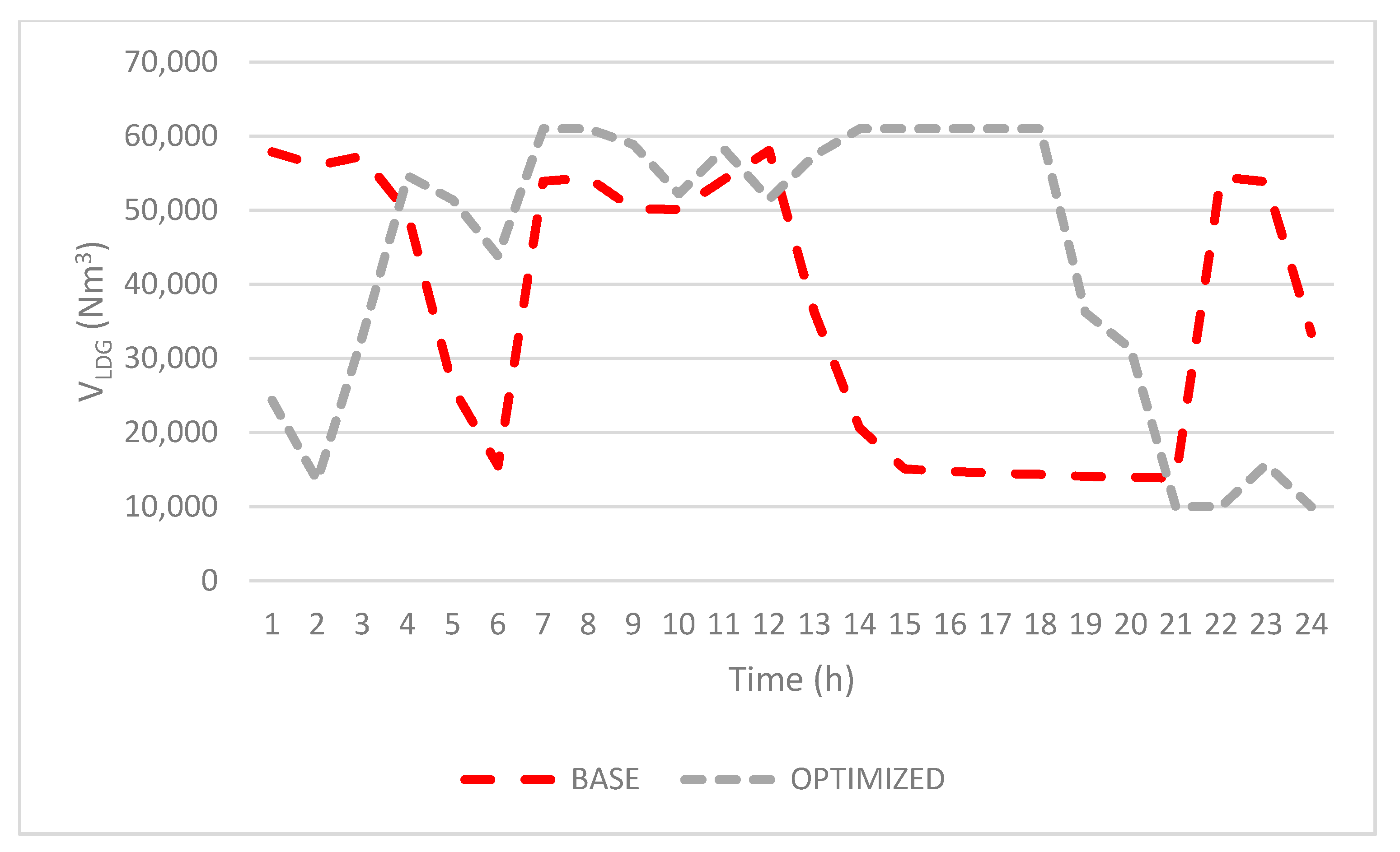
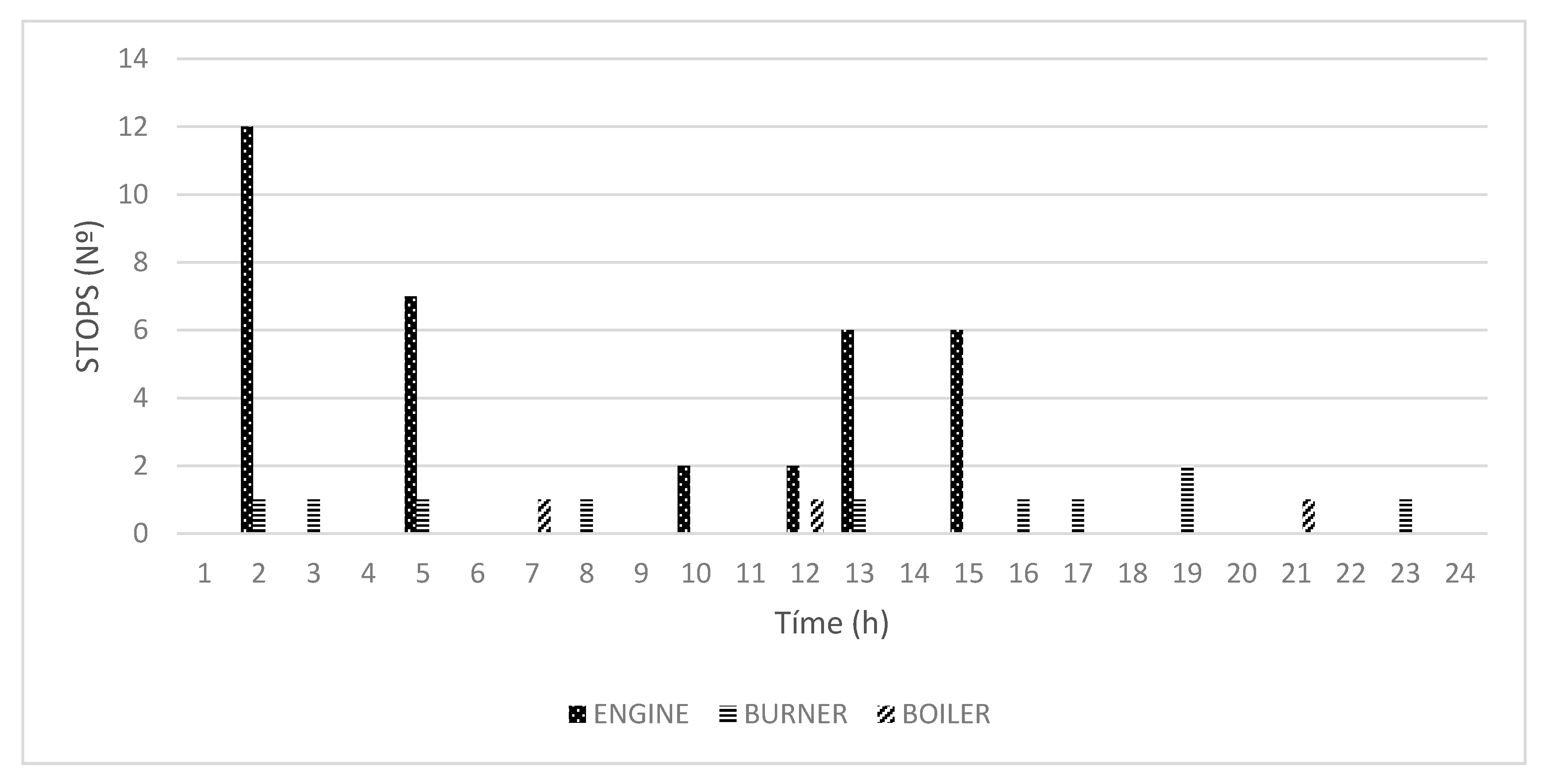
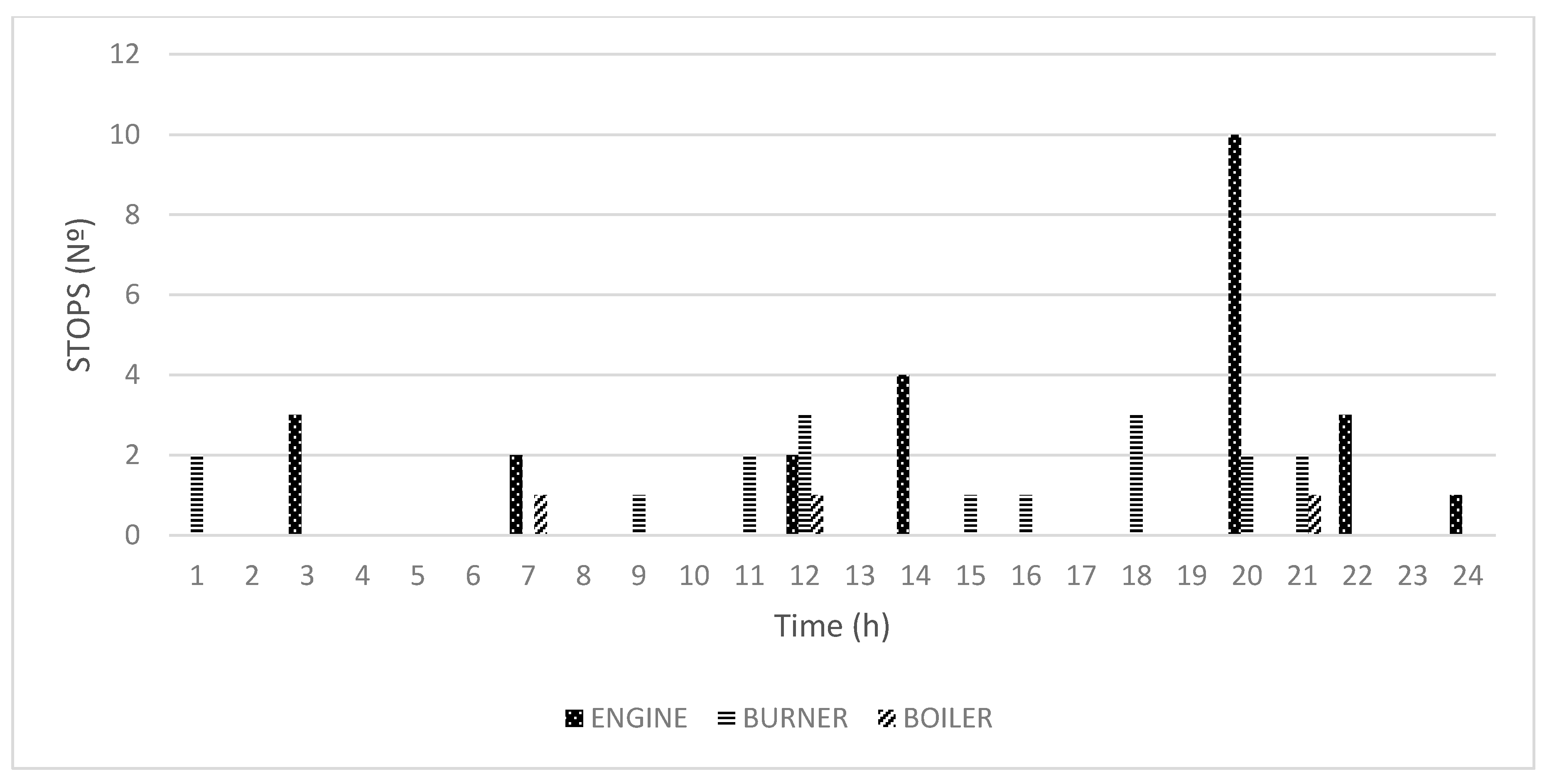
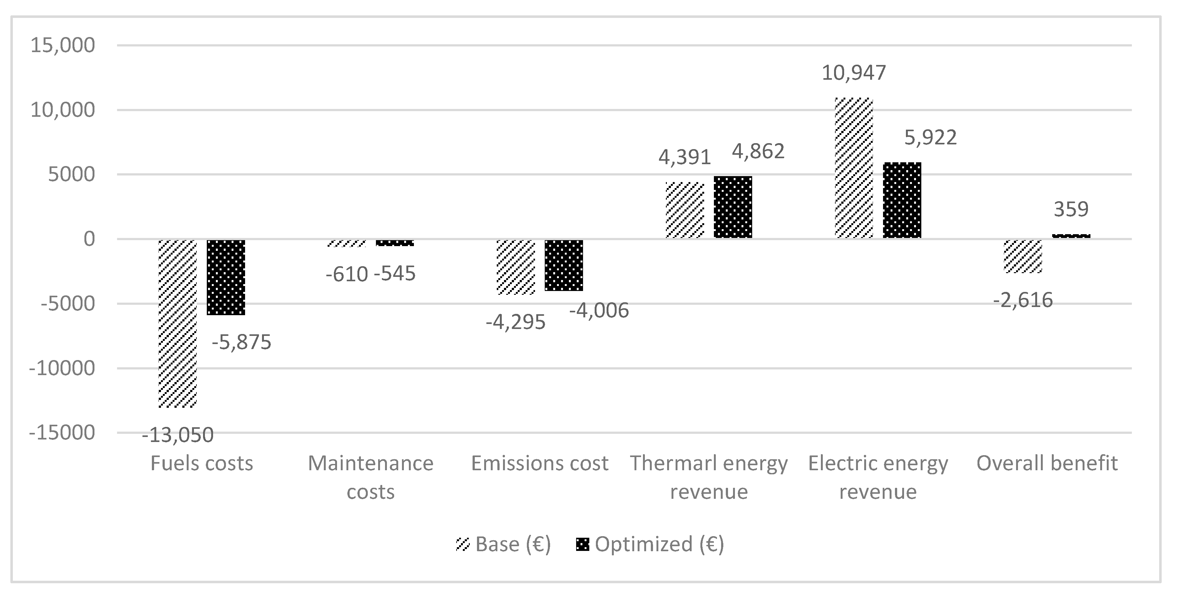
This scenario represents the base day in the operation of the plant with very irregular and discontinuous steel gas availability. The scenario involves periods of operation with natural gas due to a lack of steel gas and mixed operation with steel gas and natural gas. Thus, this scenario is interesting for comparison. Notably, steel gas is not always available depending on the operational program of the steel plant and its storage capacity, which is limited by its gasholders.

The following figures detail the initial conditions with which the different consumption strategies are evaluated. Figure 4 shows the availability of steel waste gas, and Figure 5 presents the steam requirements of the steel company. The electricity price market during this period can be seen in Figure 6.

6. Results

Here, we describe the optimization results during the period. Figure 7 and Figure 8 present the distributions of LDG, COG, and NG in the SGCP in the base scenario (based on the actual data for the studied period) and the results of the optimized solution, respectively. The base scenario refers to the 24-h situation described in Section 5.1, considering the decisions made by the managers and, thus, the outcomes produced by those decisions. That situation is taken as baseline for the comparison against the decisions proposed by the situation modelled with CPLEX. The results indicate the amount that the three kinds of gases fluctuated during the planning period. The behavior in both scenarios is very different. In the optimized solution during nighttime hours, LDG is mainly used to produce thermal energy. This is due to the low price of the electricity market (<40 €/MWh) and to avoid the consumption of NG. However, in the morning hours, the strategy is different due to the high price of the electricity market (> 55€/MWh) and the decrease in the thermal requirements of the steel factory (<50 Tn). In the afternoon (from 15 h onward), LDG accumulates in the gasometer to minimize the contribution of GN (from 19 h onwards).

As depicted in Figure 9, the volume of COG allocated to thermal production is the same in both cases (the lines are overlapped) and coincides with the amount available (Figure 4). To achieve the thermal energy requirements, NG must also be used (Figure 10). This scenario features a shortage of COG, which is complemented with NG. However, as shown in Figure 10, the consumption of NG is greater in the base case than in the optimized scenario, which yields notable savings.

Figure 11 details a comparison between the level of the base and the proposed gasholder level once the optimization is carried out. In the latter case, the optimized solution is associated at a low level during the night; however, from 4 a.m. until 6 p.m. it remains above 50,000 m³. The following hours take advantage of the energy stored in the gasholder to decrease the consumption of NG.

The numbers of engines, burners, and boilers turned on/off in the base and optimized scenarios are shown in Figure 12 and Figure 13, respectively. The optimized solution minimizes the stoppage of the motors by 29%. However, the burner changes in the boilers are increased by 70% due to the more complex management of steel gas.

Figure 14 depicts the economic results under both scenarios. The allocation proposed by the proposed model transforms a scenario with losses into a profitable scenario.

The base scenario focuses mainly on the way to avoid the consumption of NG, neglecting how more suitable off-gas allocation could contribute in a more positive way. Therefore, the base model yields higher operational costs systematically. The optimized model minimizes fuel costs by 55% based on the reduction of NG consumption. The maintenance costs are practically the same in both models. Emission costs are also lower in the proposed scenario due to the greater use of COG, which also has a much lower CO₂ emission factor than LDG. The thermal energy revenue is almost the same in both cases because the price per ton of steam produced using steel gases is the same. The revenue from the production of electrical energy is lower with the proposed model, but the overall benefits are higher.

Sensitivity Analysis

A sensitivity analysis of the most significative factors was performed. Off-gases have no cost in the present scenario. Coke batteries work in a continuous way, so their consumption is presently a priority. In the future, iron and steel plants will increase their consumption and use of steel gases, especially COG, due to its good calorific value. Therefore, COG has economic value. A sensitivity analysis of the COG price was conducted, concluding that until reaching a cost of 0.079 €/m³, the present scenario remains profitable.

Trading in the CO₂ emissions market is becoming increasingly relevant to the sustainability and competitiveness of companies. The future trend is that the price of CO₂ emissions will continue to increase. Therefore, a sensitivity analysis was conducted by increasing the P_CO2 value and comparing its process’s profitability with other very important economic parameters. One of those parameters is the capacity of the gasholder. The capacity of the gasholder is fixed, but this model could be useful to design a new process or to expand the decision-making process.

Table 9. Sensitivity analysis of the CO₂ and gasholder level.

Benefit [€]		CO2 Price (€/t)
		0	5	10	15	20
VLDG (Nm3)	30,000	4460	1019	−2422	−5864	−9306
	60,000	5387	2022	−1342	−4702	−8072
	90,000	6082	2794	−492	−3760	−7068
	120,000	6655	3444	234	−2976	−6187
	150,000	7172	4036	900	−2235	−5371

shows how the benefits vary with different amounts of CO₂ and different capacities of the gasholder. Here, the breakpoint where the cost of CO₂ emissions becomes unprofitable is projected for a specific gasholder capacity. For example, in the present scenario, a capacity of 60,000 Nm³ would be between 5 and 10 €/t. Another interesting analysis is the relationship between the gasholder capacity and the expected profit, which follows a logarithmic relationship: doubling the capacity of the gasometer does not mean doubling the profit.

Likewise,

Table 10. Sensitivity analysis of the CO₂ and thermal energy price.

Benefit [€]		CO2 Price (€/t)
		0	5	10	15	20
P TE (€/t)	2	3111	−251	−3613	−6975	−10,337
	4	5989	2626	−735	−4097	−7459
	6	8867	5504	2142	−1219	−4581
	8	11,745	8392	5020	1658	−1703
	10	14,623	11,260	7898	4536	1174

shows a comparison of thermal energy prices and CO₂ emissions. With a thermal energy price above 50% of the CO₂ price, a plant would be profitable.

7. Conclusions

The management of cogeneration processes based on off-gases in the iron and steel industry is complex. To achieve the lowest operational cost, it is important to take the entire system into account to avoid sub-optimal operations. In this paper, an MILP model for multi-period optimization of the steel gas allocation in a cogeneration system is proposed. The case study shows that the proposed method performs well in maximizing the total benefits. Compared to the base model (human decision-making), a benefit of more than 16.9% was obtained. This result is based on the operational data over one day with a shortage of off-gas and thus requires the system to be supplemented with natural gas. This is a limitation of the present study. However, this is not a rare case but a representative case of a situation that occurs with a certain frequency. In gas-sufficiency situations, human decision-making and model decision-making do not differ significantly, but when other circumstances come into play, operators tend to make decisions following short-term, and therefore less efficient, criteria. To overcome this limitation, the analysis of scenarios with a broader time horizon is proposed for further work. A 24-h time window was used because the electricity price is known anticipatedly, but scenarios with larger periods reflecting different patterns can be considered, for example a week with adverse weather conditions that entails expensive electricity prices.

Sensitivity analyses of CO₂ prices, gasholder levels, and thermal energy were also conducted. This information could be very useful when designing new cogeneration processes. In this sense, our analysis of the influence of gasometer capacity is especially important. The correct dimensioning of gasometer capacity is one of the most relevant design parameters; as noted in this study, the relation of capacity–benefits is logarithmic. The analyses of the influence of CO₂ emissions is also remarkable, as this factor is one of the most important in the context of decarbonization. This study considers only one objective because the CO₂ emissions are translated to cost in order to compute the overall profit. An interesting challenge and future line of research may be the application of multi-objective optimization in which benefits and CO₂ emissions are analyzed. As further work, a model will be developed evaluating the pareto front that relates the profit with the tons of CO₂ emissions. This, in this way, the decision makers will have valuable information for the decision-making process. The CPLEX model would enable the use of a ε-constraint multi objective approach, which is an extension of linear programming for application in bi-objective optimization problems.

References

1. World Steel Association. World Steel in Figures. 2019. Available online: https://www.worldsteel.org/en/dam/jcr:f07b864c-908e-4229-9f92-669f1c3abf4c/fact_energy_2019.pdf (accessed on 7 April 2020).
2. He, K.; Wang, L. A review of energy use and energy-efficient technologies for the iron and steel industry. Renew. Sustain. Energy Rev. 2017, 70, 1022–1039. [Google Scholar] [CrossRef]
3. Quader, M.A.; Ahmed, S.; Ghazilla, R.A.R.; Ahmed, S.; Dahari, M. A comprehensive review on energy efficient CO2 breakthrough technologies for sustainable green iron and steel manufacturing. Renew. Sustain. Energy Rev. 2015, 50, 594–614. [Google Scholar] [CrossRef]
4. Zhao, X.; Bai, H.; Hao, J. A review on the optimal scheduling of byproduct gases in steel making industry. Energy Procedia 2017, 142, 2852–2857. [Google Scholar] [CrossRef]
5. Consejería de Medioambiente y Desarrollo Rural. Principado de Asturias Información Pública—Informe Detallado SIDERGÁS|PRTR España. Available online: http://www.prtr-es.es/Informes/fichacomplejo.aspx?Id_Complejo=4919 (accessed on 25 December 2016).
6. García, S.G.; Montequín, V.R.; Fernández, R.L.; Fernández, F.O. Evaluation of the synergies in cogeneration with steel waste gases based on Life Cycle Assessment: A combined coke oven and steelmaking gas case study. J. Clean. Prod. 2019, 217, 576–583. [Google Scholar] [CrossRef]
7. Shoham, Y.; Leyton-Brown, K. Multiagent Systems: Algorithmic, Game-Theoretic, and Logical Foundations; Cambridge University Press: New York, NY, USA, 2008; ISBN 1-139-47524-X. [Google Scholar]
8. Akimoto, K.; Sannomiya, N.; Nishikawa, Y.; Tsuda, T. An optimal gas supply for a power plant using a mixed integer programming model. Automatica 1991, 27, 513–518. [Google Scholar] [CrossRef]
9. Kim, J.H.; Yi, H.; Han, C. Optimal byproduct gas distribution in the iron and steel making process using mixed integer linear programming. In Proceedings of the International Symposium on Advanced Control of Industrial Processes, Orlando, FL, USA, 2002; pp. 581–586. [Google Scholar]
10. Kim, J.H.; Yi, H.-S.; Han, C. A novel MILP model for plantwide multiperiod optimization of byproduct gas supply system in the iron-and steel-making process. Chem. Eng. Res. Des. 2003, 81, 1015–1025. [Google Scholar] [CrossRef]
11. Kim, J.H.; Yi, H.; Han, C.; Park, C.; Kim, Y. Plant-wide multiperiod optimal energy resource distribution and byproduct gas holder level control in the iron and steel making process under varying energy demands. In Computer Aided Chemical Engineering; Elsevier: Amsterdam, The Netherlands, 2003; Volume 15, pp. 882–887. ISBN 1570-7946. [Google Scholar]
12. Kong, H.; Qi, E.; Li, H.; Li, G.; Zhang, X. An MILP model for optimization of byproduct gases in the integrated iron and steel plant. Appl. Energy 2010, 87, 2156–2163. [Google Scholar] [CrossRef]
13. Qi, E.; Kong, H.; He, S. Multi-period optimal byproduct gas scheduling in iron and steel industry. Syst. Eng.-Theory Pract. 2010, 30, 2070–2079. [Google Scholar]
14. De Oliveira Junior, V.B.; Pena, J.G.C.; Salles, J.L.F. An improved plant-wide multiperiod optimization model of a byproduct gas supply system in the iron and steel-making process. Appl. Energy 2016, 164, 462–474. [Google Scholar] [CrossRef]
15. Song, J.; Zhang, A.C.; Zheng, H.K. Study on Dynamic Optimization Model of Surplus Gas Distribution in Iron and Steel Plant. Adv. Mater. Res. 2012, 610–613, 2228–2231. [Google Scholar] [CrossRef]
16. Zeng, Y.; Xiao, X.; Li, J.; Sun, L.; Floudas, C.A.; Li, H. A novel multi-period mixed-integer linear optimization model for optimal distribution of byproduct gases, steam and power in an iron and steel plant. Energy 2018, 143, 881–899. [Google Scholar] [CrossRef] [Green Version]
17. Orre, J.; Bellqvist, D.; Nilsson, L.; Alstrom, L.; Wiklund, S. Optimised Integrated Steel Plant Operation Dependent on Seasonal Combined Heat and Power Plant Energy Demand. Chem. Eng. Trans. 2018, 70, 1117–1122. [Google Scholar]
18. Pena, J.G.; de Oliveira, V.B.; Salles, J.L. Sensitivity analysis of byproduct gas distribution optimization problem in the iron and steel-making process. In Proceedings of the 2016 12th IEEE International Conference on Industry Applications (INDUSCON), Curitiba, Brazil, 20–23 November 2016; pp. 1–7. [Google Scholar]
19. Pena, J.G.C.; de Oliveira Junior, V.B.; Salles, J.L.F. Optimal scheduling of a by-product gas supply system in the iron-and steel-making process under uncertainties. Comput. Chem. Eng. 2019, 125, 351–364. [Google Scholar] [CrossRef]
20. Zhao, X.; Bai, H.; Shi, Q.; Han, J.; Li, H. Optimal distribution of byproduct gases in iron and steel industry based on mixed integer linear programming (MILP). In Energy Technology 2015; Springer: Berlin/Heidelberg, Germany, 2015; pp. 73–80. [Google Scholar]
21. Zhao, X.; Bai, H.; Shi, Q.; Lu, X.; Zhang, Z. Optimal scheduling of a byproduct gas system in a steel plant considering time-of-use electricity pricing. Appl. Energy 2017, 195, 100–113. [Google Scholar] [CrossRef]
22. Manual, C.U. IBM ILOG CPLEX Optimization Studio. Version 1987, 12, 1987–2018. [Google Scholar]
23. Bixby , R.E. A brief history of linear and mixed-integer programming computation. Doc. Math. 2012, 107–121. [Google Scholar]
Figure 1. Schematic view of a simple iron and steel cogeneration process.
Energies 13 03781 g001
Figure 2. Schematic view of the thermal plant.
Energies 13 03781 g002
Figure 3. Schematic view of the electrical plant.
Energies 13 03781 g003
Figure 4. Availability of steel waste gas in the planning period.
Energies 13 03781 g004
Figure 5. Process steam demand.
Energies 13 03781 g005
Figure 6. Electricity market price.
Energies 13 03781 g006
Figure 7. Base and optimized LDG distribution for electricity production in the planning period.
Energies 13 03781 g007
Figure 8. Base and optimized distribution LDG for steam production in the planning period.
Energies 13 03781 g008
Figure 9. Base and optimized distribution COG for steam production in the planning period.
Energies 13 03781 g009
Figure 10. Base and optimized distribution NG for steam production in the planning period.
Energies 13 03781 g010
Figure 11. Base and optimized VLDG in the gas holder.
Energies 13 03781 g011
Figure 12. Base engine, burner, and boiler ON/OFF.
Energies 13 03781 g012
Figure 13. Optimized engine, burner, and boiler ON/OFF.
Energies 13 03781 g013
Figure 14. Comparative break down of the base and optimized benefits.
Energies 13 03781 g014