A Novel Strategy to Reduce Computational Burden of the Stochastic Security Constrained Unit Commitment Problem

Abstract

The uncertainty related to the massive integration of intermittent energy sources (e.g., wind and solar generation) is one of the biggest challenges for the economic, safe and reliable operation of current power systems. One way to tackle this challenge is through a stochastic security constraint unit commitment (SSCUC) model. However, the SSCUC is a mixed-integer linear programming problem with high computational and dimensional complexity in large-scale power systems. This feature hinders the reaction times required for decision making to ensure a proper operation of the system. As an alternative, this paper presents a joint strategy to efficiently solve a SSCUC model. The solution strategy combines the use of linear sensitivity factors (LSF) to compute power flows in a quick and reliable way and a method, which dynamically identifies and adds as user cuts those active security constraints $N-1$ that establish the feasible region of the model. These two components are embedded within a progressive hedging algorithm (PHA), which breaks down the SSCUC problem into computationally more tractable subproblems by relaxing the coupling constraints between scenarios. The numerical results on the IEEE RTS-96 system show that the proposed strategy provides high quality solutions, up to 50 times faster compared to the extensive formulation (EF) of the SSCUC. Additionally, the solution strategy identifies the most affected (overloaded) lines before contingencies, as well as the most critical contingencies in the system. Two metrics that provide valuable information for decision making during transmission system expansion are studied.

1. Introduction

The security constrained unit commitment (SCUC) problem is the optimization model that schedules a set of power generation units to meet an expected energy demand over a typical time horizon of 24 h while meeting several system constraints (e.g., operational limits of the generation units and transmission limits) under normal operating conditions and also under $N-1$ contingencies. The SCUC problem is widely used in day ahead and real time markets to obtain an economically, reliably, and safely operation of the power system [1]. The SCUC is a complex mixed integer programming (MIP) problem since it belongs to the class of NP-hard problems [2]. This feature has challenged researchers to approach the complexity of the SCUC problem in different ways when dealing with large-scale power systems. Examples of these solution approaches include Lagrangian relaxation (LR) and Benders decomposition (BD) techniques, which have been implemented to solve the SCUC model in efficient computing times [3,4,5,6,7]. Dealing with $N-1$ security constraints posses a challenge when solving the SCUC problem. Therefore, several authors have proposed different alternatives to tackle them. In [8], the authors defined necessary and sufficient conditions to identify and eliminate inactive $N-1$ security constraints. Similarly, H. Wu et al. [9] presented analytical feasibility conditions to define only the subset of security constraints of the SCUC problem feasible region. Likewise, in [10], the authors mathematically ruled out unnecessary security constraints using again necessary and sufficient conditions. However, the application of these methods could be limited for large-scale practical problems, and therefore decomposition techniques such as BD should be required in a complementary manner [9,10]. On the other hand, some authors have addressed this challenge without relying to decomposition techniques or any of the previously mentioned methods. This is the case of Capitanescu et al. [11] who developed a preventive security-constrained optimal power flow (PSCOPF) defining two constraint filtering techniques under the concepts of dominated and non-dominated constraints. Including only the latter in the PSCOPF model accelerates its solution time.

Currently, a key factor to reduce the computing times when solving the SCUC problem is the use of linear sensitivity factors (LSFs) to model the power grid. The Power Transfer Distribution Factor (PTDF) and the Line Outage Distribution Factor (LODF) estimate power flows changes under power injection variations in buses and line outages (i.e., $N-1$ contingencies), respectively [12]. Nonetheless, Eslami et al. [13] proposed a new method for reducing SCUC variables and constraints under a conventional formulation of the power grid for post-contingency constraints. Several iterative methodologies based on LSFs have been developed to increase the computational efficiency of SCUC models for large-scale power systems. In [2], the authors added only binding $N-1$ security constraints to the SCUC problem using the Gurobi deferred constraints function (i.e., lazy constraints). Similarly, Marín-Cano et al. [14] proposed the implementation of user cuts to improve the computational performance of the SCUC and presented indices that provide expansion signals for the transmission network. Xavier et al. [15] added effective security constraints based on the concept of priority queue, adding at most only one $N-1$ security constraint per line. All these methodologies aim to generate iteratively the feasible region of the SCUC problem reducing effectively the computation times needed to solve this problem. However, it is noteworthy that none of the aforementioned methodologies has been applied in the analysis of the safe operation of electrical systems under uncertainty [16].

Recently, the evolution of power systems has imposed major challenges in the solution of the SCUC due to the uncertainty caused by the integration of large amounts of intermittent renewable resources. One way to address these challenges is through the SSCUC problem [17]. In [18], the authors evaluated security through a multi-stage stochastic programming model where random system disturbances (generation unit and transmission line failures) are modeled through scenario trees. To solve the SSCUC, they decomposed the problem using LR. The authors of [19] used BD to solve a SSCUC considering the intermittency and volatility of wind generation through scenarios. Two different procedures to tackle the SSCUC are compared in [17]. The first one is based on scenarios, whereas the second one is based on optimization intervals. The SSCUC model presented in [20] considers wind power production scenarios and non-spinning reserves. The authors relied on chance-constrained programming to solve this variant of the SSCUC. Similarly, the authors of [21] studied an $N-1$ security and chance-constrained unit commitment (SCCUC) model. They formulated this SCCUC problem as a mixed-integer second-order cone program with two types of reserves to consider wind fluctuations and single component outages (i.e., generators or transmission lines outages). In [22], the authors relied on BD to solve a SSCUC model considering different types of pumped-storage hydropower plants. Finally, Park et al. [23] modeled a SSCUC using two-stage stochastic programming, considering dynamic line rating to improve the use of transmission lines during $N-1$ conditions.

The above references highlight the importance of the SSCUC models as a way to hedge against uncertainty in the safe operation of power systems. However, it should be pointed out that high computational speed is of great importance for operators at the moment of real-time decision-making, since the mathematical models for UC under uncertainty are computationally much more complex than their deterministic counterparts [24]. To the best of our knowledge, there are few studies that address the computational complexity of the SSCUC problem and focus on solving the problem quickly and effectively. Among them, Wang and Fu [1] proposed a fully parallel stochastic SCUC approach to obtain efficient and fast solutions in large-scale electrical systems and N. Yang et al. [25] proposed a method that aims to improve the efficiency of the SSCUC problem under constrained ordinal optimization (COO). This approach has two advantages: The first one is a recognition of discrete variables to reduce the solution space of the approximate COO rough model. The second one is the inclusion of a strategy to reduce non-effective security constraints, as presented in [26], which in turn is based on the analytical conditions proposed in [8].

Following the authors of [1,25], in this work, we propose a novel and easy-to-implement strategy to efficiently solve a SSCUC problem under the uncertainty of large penetration of intermittent energy sources. This strategy has the following features: (i) it uses sensitivity linear factors to compute power flows to reduce the number of variables and constraints when compared to conventional network modeling; (ii) it considers user cuts to dynamically add active $N-1$ security constraints, as proposed in [14]; and (iii) it uses the PHA decomposition algorithm to relax the SSCUC model. As shown in [27], the PHA is able to achieve high-quality solutions for stochastic optimization in large-scale power systems. As an additional result from the proposed strategy, we define several indices that allow identifying the most critical and vulnerable lines in terms of the overloads they cause or suffer under single contingencies. Such information is useful to the system planner for short-term transmission expansion analyses.

The rest of the paper is organized as follows. Section 2 introduces some preliminary background on stochastic optimization and presents the SSCUC model studied in this paper. Section 3 presents the elements of the solution strategy proposed in the paper as well as the general framework that embeds $N-1$ security cuts into the progressive hedging algorithm. Section 4 includes the results of the evaluation of the proposed strategy in the IEEE RTS-96 test system. Section 5, introduces and exemplifies transmission expansion indices calculated with the results of the proposed strategy. Finally, Section 6 concludes the paper and provides additional research extensions.

2. Stochastic SCUC Formulation

In this section, we model the SSCUC problem as a two-stage stochastic program. We first set the scene for this by introducing some important background on stochastic optimization, and then we introduce the detailed SSCUC model. For easy reference, Appendix A presents the nomenclature used in the modeling of the SSCUC.

2.1. Background

Stochastic models to address the SCUC problem have been widely used by system operators, especially when wind generation is considered [1]. From a mathematical point of view, the SSCUC problem can be formulated as a two-stage stochastic MIP problem based on scenarios. In the first stage, the generation units are committed, while, in the second (uncertainty) stage, the power output level of each generator to meet the demand is decided, taking into account the $N-1$ criterion. In sum, the SSCUC problem aims to minimize the expected operation cost (Equation (1)), while satisfying the generation and transmission constraints in all scenarios ($\xi \in \Xi$). The SSCUC problem represented through its extensive form (EF) follows:

$$\underset{x,y\left(\xi \right)}{\mathrm{Min}}{c}^{T}x+\sum _{\xi =1}^{\Xi }{p}_{\xi }d{\left(\xi \right)}^{T}y\left(\xi \right)$$

(1)

$$s.t.Ax\le b$$

(2)

$$T\left(\xi \right)x+W\left(\xi \right)y\left(\xi \right)\le h\left(\xi \right)\forall \xi \in \Xi$$

(3)

The decision variable x of the first stage represents the on/off state of a generator (i.e., its commitment), whch is implicitly independent of the realization of the scenarios ($\xi$) [28]. The decision variable of the second stage $y\left(\xi \right)$ represents the power dispatched by each generation unit in each scenario ($\xi$) (with probability $p_{\xi }$ for $\xi \in \Xi$). Equations (2) and (3) represent the constraints associated with the first and second stage, respectively. A is the matrix of coefficients associated with variable x. The coefficients c and d are the costs associated with the binary variable x and the continuous variable y, respectively.

An alternative representation of the SSCUC problem is through the Extensive Form of the Scenario (EFS) as follows:

$$\underset{x\left(\xi \right),y\left(\xi \right)}{\mathrm{Min}}\sum _{\xi =1}^{\Xi }{p}_{\xi }[c^{T}x\left(\xi \right)+d{\left(\xi \right)}^{T}y\left(\xi \right)]$$

(4)

$$s.t.Ax\left(\xi \right)\le b$$

(5)

$$T\left(\xi \right)x\left(\xi \right)+W\left(\xi \right)y\left(\xi \right)\le h\left(\xi \right)\forall \xi \in \Xi$$

(6)

$$p_{\xi }x\left(\xi \right)-p_{\xi }\widehat{x}=0\forall \xi \in \Xi$$

(7)

Unlike Equations (1)–(3), in Equations (4)–(7) the variables of the first stage are calculated for each realization of the scenario ($\xi$). Additionally, it includes (7), known as the non-anticipativity constraint, which requires that the variable x does not depend on the scenarios for all feasible solutions [28].

2.2. Mathematical Model of the SSCUC Problem

The first and second stages of the SSCUC are based on the formulation and modeling in [29,30], respectively. Constraints of the first stage include binary variable logical implications, start-up and shut down costs and minimum down and up time. On the other hand, constraints of the second stage consider minimum and maximum generator outputs as well as ramping and transmission limits. Contrary to H. Pandžić et al. [29], the formulation of transmission constraints uses LSF, PTDF for normal operation and LODF for operation under $N-1$ line contingencies. Details of the LSF calculation are provided in [2,14].

The objective function of the SSCUC minimizes the expected value of the operating costs of the system, consisting on the costs of the generation of thermal plants $C_i(t,\xi )$, the costs associated with the variable of involuntary load shedding $L_s^{sh}(t,\xi )$ and the costs associated with wind power curtailment $Q_w(t,\xi )$. This objective function is subject to the constraints given by (9)–(30), as shown below. Equations (9)–(24) are well-known constraints of the UC formulation that can be found in classical references of this problem (e.g., [29]). We add to this formulation net-power balance equations (constraints (25) and (26)), involuntary load shedding (constraint (29)) and wind power curtailment (constraint (30)). Remarkably, the constraints in Equation (27) and (28) resort to the PTDF and LODF to reduce the complexity of modelling the pre- and post-contingency power flows on lines.

$$Min\sum _{\xi =1}^{\Xi }{p}_{\xi }·[\sum _{t=1}^T\sum _{i=1}^I{C}_i(t,\xi )+\sum _{t=1}^T\sum _{s=1}^S{c}^{sh}·L_s^{sh}(t,\xi )+\sum _{t=1}^T\sum _{w=1}^W{c}_{\omega }·Q_w(t,\xi )]$$

(8)

This objective function is subject to the constraints given by (9)–(30).

• Binary variable logic:

  $$y_i\left(t\right)-z_i\left(t\right)=x_i\left(t\right)-x_i(t-1)\forall t\le T,i\le I$$

  (9)

  $$y_i\left(t\right)+z_i\left(t\right)\le 1\forall t\le T,i\le I$$

  (10)
• Operating costs of thermal plants:

  $$C_i(t,\xi )=a_i{x}_i\left(t\right)+\sum _{b=1}^B{k}_{i,b}{g}_{i,b}(t,\xi )+{SUC}_i\left(t\right)\forall t\le T,i\le I,\xi \le \Xi$$

  (11)
• Total power output of the thermal generator i, expressed as the total sum of the generation level in each segment b of the cost curve:

  $$g_i(t,\xi )=\sum _{b=1}^B{g}_{i,b}(t,\xi )\forall t\le T,i\le I,\xi \le \Xi$$

  (12)
• Minimum generator output constraint:

  $$g_i(t,\xi )\ge g_i^{min}{x}_i\left(t\right)\forall t\le T,i\le I,\xi \le \Xi$$

  (13)
• Maximum generator output constraint:

  $$g_{i,b}(t,\xi )\le g_i^{max}{x}_i\left(t\right)\forall t\le T,i\le I,b\le B,\xi \le \Xi$$

  (14)
• Initial on–off status of generator i at $t=0$ (15), minimum up (16) and down time constraints (17):

  $$x_i\left(t\right)=g_i^{on--off}\forall i\le I,t\le L_i^{up,min}+L_i^{down,min}$$

  (15)

  $$\sum _{tt=t-g_i^{up}+1}^t{y}_i\left(tt\right)\le x_i\left(t\right)\forall i\le I,\forall t\ge L_i^{up,min}$$

  (16)

  $$\sum _{tt=t-g_i^{down}+1}^t{z}_i\left(tt\right)\le 1-x_i\left(t\right)\forall i\le I,\forall t\ge L_i^{down,min}$$

  (17)

  where

  $$L_i^{up,min}=min[T,(g_i^{up}-g_i^{up,init})g_i^{on--off}]$$

  $$L_i^{down,min}=min[T,(g_i^{down}-g_i^{down,init})(1-g_i^{on--off})]$$
• Ramping constraints:

  $$-{ramp}_i^{down}\le g_i(t,\xi )-g_i(t-1,\xi )\forall i\le I,2\le t\le T,\xi \le \Xi$$

  (18)

  $${ramp}_i^{up}\ge g_i(t,\xi )-g_i(t-1,\xi )\forall i\le I,2\le t\le T,\xi \le \Xi$$

  (19)

  $$-{ramp}_i^{down}\le g_i(t=1,\xi )-g_i^0\forall i\le I,\xi \le \Xi$$

  (20)

  $${ramp}_i^{up}\ge g_i(t=1,\xi )-g_i^0\forall i\le I,\xi \le \Xi$$

  (21)
• Generator off counter set-up constraints. In this case, symbols | and $\wedge$ indicate the logical conditions IF and AND, respectively:

  $$\begin{array}{cc}\hfill w_{i,j}\left(t\right)\le & \sum _{tt=SU{C}_{i,j}^{lim}}^{min\{t-1,SU{C}_{i,j+1}^{lim}-1\}}{z}_i(t-j)\hfill \\ \hfill & +1\left|\right\{j=J-1\wedge SU{C}_{i,j}^{lim}\le g_i^{down,init}+t-1<SU{C}_{i,j+1}^{lim}\}\hfill \\ \hfill & +1\left|\right\{j=J\wedge SU{C}_{i,j}^{lim}\le g_i^{down,init}+t-1\}\forall t\le T,i\le I,j\le J\hfill \end{array}$$

  (22)

  $$\sum _{j=1}^J{w}_{i,j}\left(t\right)=y_i\left(t\right)\forall t\le T,i\le I$$

  (23)

  $${SUC}_i\left(t\right)=\sum _{j=1}^J{w}_{i,j}\left(t\right)\forall t\le T,i\le I$$

  (24)
• Net power balance constraints:

  $$P_s^{Net}(t,\xi )=\sum _i{A}_i^s·g_i(t,\xi )-D_s\left(t\right)+L_s^{sh}(t,\xi )+\sum _w{A}_w^s·[{\widehat{g}}_w(t,\xi )-Q_w(t,\xi )]$$

  (25)

  $$\forall ,s\le S,t\le T,\xi \le \Xi$$

  $$\sum _s{P}_s^{Net}(t,\xi )=0\forall t\le T,\xi \le \Xi$$

  (26)
• Power flow constraints under normal (27) and post-contingency (28) operation conditions. In this case, ${\overline{PTDF}}_{l,s}$ is the power transfer distribution factor of line l for a power injection at bus s, and ${\overline{LODF}}_{l,k}$ is the line outage distribution factor for line l when line k is out of service.

  $$-F_l^{\max }·TCF\le \sum _s{\overline{PTDF}}_{l,s}·P_s^{Net}(t,\xi )\le F_l^{\max }·TCF\forall l\le L,t\le T,\xi \le \Xi$$

  (27)

  $$-F_l^{max}·TCF\le F_l(t,\xi )+{\overline{LODF}}_{l,k}·F_k(t,\xi )\le F_l^{max}·TCF\forall l\le L,k\le K,t\le T,\xi \le \Xi$$

  (28)
• Constraints (29) and (30), represent the limit of involuntary load shedding $L_s^{sh}(t,\xi )$ and wind power curtailment $Q_w(t,\xi )$, respectively:

  $$0\le L_s^{sh}(t,\xi )\le D_s\left(t\right)\forall s\le S,t\le T,\xi \le \Xi$$

  (29)

  $$0\le Q_w(t,\xi )\le {\widehat{g}}_w(t,\xi )\forall w\le W,t\le T,\xi \le \Xi$$

  (30)

3. Solution Strategy

The proposed solution strategy embeds the dynamic generation of $N-1$ security constraints into the PHA. We first describe these two elements independently and then present the embedding procedure.

3.1. Method for Adding Binding N − 1 Security Constraints

LODFs allow the modeling of $N-1$ contingencies with low computational cost [2,12,14]. From the standpoint of computational efficiency, it makes no sense to consider all possible $N-1$ contingencies, since not all of them generate violations on the maximum thermal transmission limit of the rest of system lines. Therefore, to take into account only the binding $N-1$ security constraints that define the feasible region of the SCUC problem, we follow the method proposed by Marín-Cano et al. [14]. Such approach is based on the concept of user cuts. These cuts are linear constraints strategically and dynamically added by the user, based on the implicit information of the problem [31], with the objective of tightening model (8)–(30).

Algorithm 1 shows the method proposed by Marín-Cano et al. [14] to add (only) sufficient and necessary $N-1$ constraints to the model through user cuts. In Step 1, the $SC{R}_{l,k,t}\left(\xi \right)$ parameter is set to zero to discard the $N-1$ security constraints (28), since the objective is to solve only the base case (normal operation) of the system during the first iteration of the process. In the main loop (Steps 2–14), the model defined by Equations (8)–(30) is solved iteratively (Step 3). This process, Steps 4–9, estimates useful parameters that allow finding those $N-1$ security constraints directly linked to the feasible region of the SSCUC problem. In Step 4, parameter $O{P}_{l,k,t}\left(\xi \right)$ is reset to zero, with the aim of storing the overload value of only new $N-1$ security constraints. In Step 5, the parameter ${\widehat{F}}_{l,k}(t,\xi )$ estimates the post-contingency power flows of the lines based on the optimal flows in the normal operating state of the line l and the contingency k, which are $F_l^{\ast }(t,\xi )$ and $F_k^{\ast }(t,\xi )$, respectively. These values were previously calculated in Step 3. Once ${\widehat{F}}_{l,k}(t,\xi )$ is estimated, Step 6 compares it with the maximum transmission capacity for each line $F_l^{max}$. If this capacity is surpassed, Step 8 calculates and stores the values of the overloads generated at the lines in parameter $O{P}_{l,k,t}\left(\xi \right)$. Furthermore, the sum of this parameter allows calculating the total system overload $TO$ in Step 9. This value is useful to define the stopping condition of the algorithm (Step 12). In Step 10, the addition of $N-1$ security constraints (28) is performed, for combinations of $l,k,t,\xi$ where $SC{R}_{l,k,t}\left(\xi \right)$ is equal 1; this last parameter allows to record and count all the overloads in each iteration. In Step 12, if there have been no overloads since the first iteration of the algorithm, then $O{P}_{l,k,t}\left(\xi \right)$ is zero, thus $TO=0$. Step 14 is the end of the iterative process when $TO$ is zero or less than a tolerance value $tol$; in this case, we set $tol=1^{-7}MW$. For a detailed description of this method, the interested reader is referred to [14].

Algorithm 1: Method for Adding N − 1 Security Constraints.

1. Set: $SC{R}_{l,k,t}\left(\xi \right)=0,\forall l\le L,k\le K,t\le T,\xi \le \Xi$

3.2. Progressive Hedging Algorithm

The extensive form of a stochastic optimization problem consists of a single mathematical model where all constraints are written for all possible scenarios [32]. For large-scale problems, such formulation does not guarantee a solution due to the lack of computational resources [32]. As a solution alternative, PHA is a scenario-based decomposition method initially proposed by Rockafellar and Wets [33]. In PHA, the stochastic problem is solved independently scenario by scenario, by relaxing the non-anticipativity constraint. This decomposition obtains good solutions with high computational efficiency [28]. Furthermore, PHA has proven to be much more stable than other widely used algorithms in the literature such as BD [32,34]. For these reasons, PHA has recently been used as a promising solution method for the stochastic operation of electrical power systems, such as unit commitment [27,32,35,36,37] and the short- and medium-term hydro-thermal planning [34,38]. Algorithm 2, taken from Gade et al. [28], describes the PHA for two-stage Stochastic MIP problems. In PHA, $\rho$ is a penalty (scalar or vector) of the same length of the non-anticipativity variable x [28,32]. In Step 1, the iteration counter $\nu$ and weight vector $w^0\left(\xi \right)$ are initialized. In Steps 2–4, the initial solution of the subproblems of each scenario is obtained. Step 5 updates the iteration counter $\nu$. In Step 6, the algorithm defines the current best estimate of a non-anticipativity solution (${\overline{x}}^{\nu }$) that does not depend on the realization of scenario $\xi$. Step 7 estimates multipliers $w\left(\xi \right)$ that are used to update the non-anticipativity condition. In Steps 8–10, the multipliers $w\left(\xi \right)$ are used together with a proximal term ($\frac{\rho }{2}{\Vert x-{\overline{x}}^{\nu }\Vert }^2$) to find an optimal solution when the x values do not depend on the scenarios. The main loop (Steps 5–10) is repeated until the convergence condition is met (Step 11).

Algorithm 2: Progressive Hedging Algorithm.

1 initialize: $\nu =0,w^{\nu }\left(\xi \right)=0,\forall \xi \in \Xi$

11 if$x\left(\xi \right)$ is the same for all scenarios $\xi \in \Xi$then stop and report ${\overline{x}}^{\nu }$;$\phantom{(}$

12 else go to 5;$\phantom{(}$

3.2.1. Adjustment of $\rho$ Parameter and Convergence Improvement

As reported in [39,40], an important factor for the performance of the PHA is its high sensitivity to the value of the penalty parameter $\rho$. This parameter determines the step length of the W dual price update, and its inappropriate choice could lead to non-convergence or slow convergence times [32]. Currently, there is no general rule for the selection of $\rho$ based on theoretical analysis [40]. However, high values of $\rho$ could give faster convergence rates in Lagrangian methods [39]. An adaptive method, as well as a comprehensive summary of the different strategies for the adjustment of $\rho$ can be found in [40].

Different strategies for adjusting the penalty factor $\rho$ have been used when dealing with the stochastic UC problem. The authors of [27] used a value of $\rho$ proportional to the hedging variable (i.e., $\rho$ is proportional to the cost of the on/off state variables). An adjustment of $\rho$ based on locational marginal prices for different nodes and time periods was proposed by Ryan et al. [32]. Alternatively, Li et al. [35] proposed a method for using the shadow prices of the coverage variable as a penalty factor $\rho$. Finally, Ordoudis et al. [36] defined a new way of adjusting $\rho$ as a fraction of the objective function proportional to the cost of the hedging variable averaged over all scenarios.

Additionally, the cyclic behavior of the PHA does not guarantee convergence while solving the Stochastic UC problem, due to the binary nature of the on/off state variables. To tackle this problem, some heuristic variable setting procedures have been proposed to improve the convergence speed of the PHA [27,35]. In this work, we follow the rounding technique proposed by Li et al. [35] to guarantee convergence at the end of the PHA. Setting $\overline{x}$ when its value is close to 0 or 1, this rounding technique has proven to be flexible, easy to implement, and it has been used successfully by other authors [36]. In this technique, two thresholds values ($\alpha ,\beta$) define three categories to round the value of $\overline{x}$, as follows:

$${\overline{\mathbf{x}}}^{\mathit{round}}=\left\{\begin{array}{cc}1& \mathrm{if}\overline{x}\ge 1-\alpha \\ 0& \mathrm{if}\overline{x}\le \beta \\ x\in \{0,1\}& \mathrm{if}\beta <\overline{x}<1-\alpha \end{array}\right.$$

(31)

Although this rounding technique can speed-up the computation time of the PHA, it could also generate infeasibility [35]. To avoid this behavior, threshold values of $\beta$ must be adjusted close to 0 to guarantee enough availability of powered-up units within the system [35,36]. On the other hand, $\alpha$ can be chosen with more flexibility since a large availability of power units guarantees feasibility.

3.3. Integrating N − 1 Security Constraints Within the PHA

As a novel and effective strategy to address the computational challenge imposed by the SSCUC problem, Algorithm 3 shows the integration of the iterative method proposed by Marín-Cano et al. [14] within the PHA.

Algorithm 3: Method for Adding $N-1$ Constraints Embedded Within the PHA.

1 Set:    $SC{R}_{l,k,t}\left(\xi \right)=0$, $\forall l\le L,k\le K,t\le T,\xi \le \Xi$

2 Initialize:$\nu =0,w^{\nu }\left(\xi \right)=0,{\rho }^0=0,\overline{x}=0,\forall \xi \in \Xi$

3 Update Iteration:$\nu =\nu +1$

19 Compute:${\overline{x}}^{\nu }$ = ${\sum }_{\xi \in \Xi }{p}_{\xi }\left(x^{\nu }\right)$

20 Update:${\rho }^{\nu }$ according to the strategies presented in Section 3.2.1

21 Update:$w^{\nu }\left(\xi \right)=w^{\nu }\left(\xi \right)+\rho (x^{\nu }\left(\xi \right)-{\overline{x}}^{\nu })$, $\forall \xi \in \Xi$

22 if$x\left(\xi \right)$ is equal in every scenario $\xi$then stop and report ${\overline{x}}^{\nu }$;$\phantom{(}$

22 else go to 3;$\phantom{(}$

Steps 1 and 2 initialize the necessary working parameters for the $N-1$ constraint addition method and for the PHA, respectively. Step 3 updates the iteration for the main iterative process of the PHA where every sub-problem of each scenario (Step 4) is solved. Steps 5–17 account for the proposed $N-1$ security constraint addition method, which is embedded within the iterative PHA process. Here, $x^{\nu }\left(\xi \right)$ represents the hedging variable of PHA in each iteration $\nu$ and each scenario $\xi$. In this case, the hedging variable is the binary variable ($x\in \{0,1\}$) that assigns the on/off status of each generation unit. Once a solution for each scenario has been found through the $N-1$ cut-adding method (Step 17), Steps 18–20 are the continuation of the PHA to find an optimal solution $x^{\nu }\left(\xi \right)$ for all scenarios meeting the non-anticipativity condition (Step 19), and the penalty factor (Step 20) and weight updating procedures (Step 21), respectively. It is important to note that, to improve the PHA convergence, in Step 20, the penalty factor ${\rho }^{\nu }$ is updated in every PHA iteration $\nu$, according to the strategies presented in Section 3.2.1. The procedure stops when the stopping condition (convergence of x) is met and the value ${\overline{x}}^{\nu }$ reported (Step 21).

4. Results

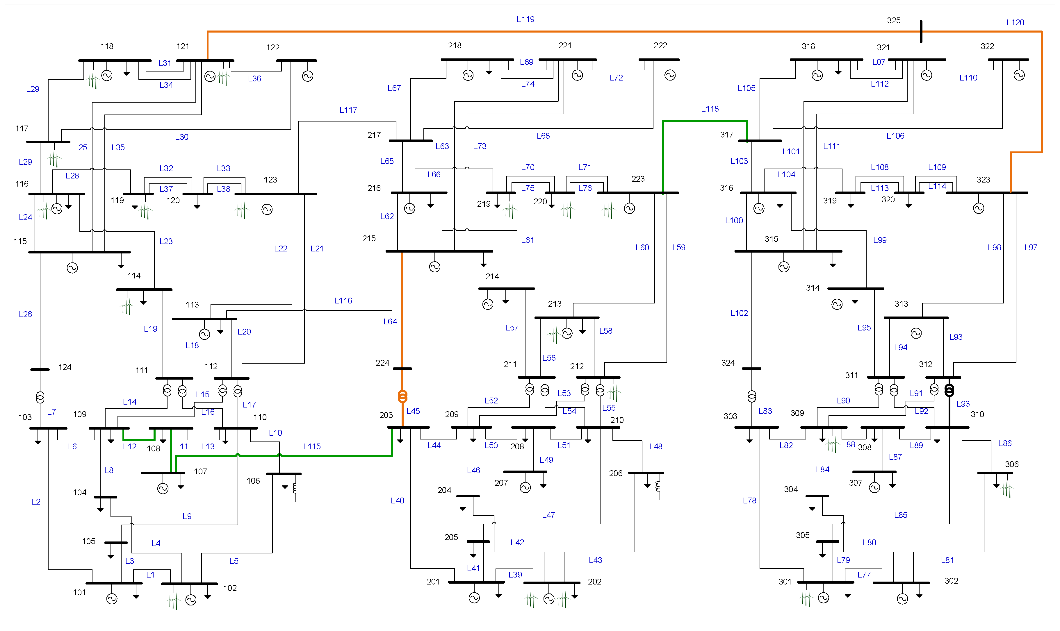
The test system used to evaluate the proposed strategy is the IEEE RTS-96 (see Figure 1) used previously whose information is fully available in [30]. This system is made up of 73 buses, 120 transmission lines, 96 thermal generators, and 19 wind farms (with an installed capacity of 6900 MW and located at buses 102, 114, 116, 118, 121, 119, 123, 202, 212, 213, 219, 220, 223, 301, 306 and 309. There are 51 loads with a maximum demand of 7539 MW and an average demand of 6258 MW. A time horizon of 24 h is considered. The SSCUC problem for this system considers 10 scenarios each with a given probability representing different generation outputs of the wind farms throughout the 24 h of the day. A detailed description of the scenarios under consideration, as well as the Excel sheets containing all input data, can be consulted in [30].

The proposed computational strategy was tested on two computers: an Intel Xeon E5 @ 2.40GHz server with 44 cores and 256 GB of RAM memory (hereafter, server) and an Intel Core i7 @ 3.4GHz desktop computer with 8 cores and 8 GB of RAM memory (hereafter, desktop). The proposed approach was implemented using the commercial algebraic modeling system GAMS version 24.8.5, with CPLEX V12.6.1 as optimization engine.

4.1. Parameters Setting for the PHA

One of the first parameters to be adjusted is the penalty factor $\rho$. Values of $\rho$ based on energy production costs of the hedging variable are suggested as a good option to foster the convergence of the PHA [36]. Additionally, we selected two of the updating strategies cited in Section 3.2.1: ${\rho }_1$ is the strategy proposed by Watson and Woodruff [27], whereas ${\rho }_2$ is the one proposed by Ordoudis et al. [36].

Another important factor is the selection of the hedging variable. Some authors have carried out experiments to study which is the best hedging variable within the Stochastic UC problem [35,36]. Under different adjustment strategies of $\rho$, Ordoudis et al. [36] showed that the best-performing hedging variable is the on/off status variable, rather than the start and stop down variable. Accordingly, in our computational experiments, we used as hedging variable the on/off state variable ($x\in \{0,1\}$).

Finally, to guarantee convergence and feasible PHA solutions in the different tests of the proposed computational strategy, we set parameters $\alpha$ and $\beta$ in the context of the so-called rounding technique. It is advisable to assign 0 to $\beta$ to guarantee whole availability of generation units to have a higher chance of reaching feasibility as mentioned in [35,36]. On the other hand, $\alpha$ must be set for every problem. In this case, an initial value of $\alpha$ is set and small variations over this value are performed. As illustrated in [36], small increments of $\alpha$ can provide high quality solutions in short PHA running times. Therefore, in our experiments, we set $\beta$ to zero, and the values of $\alpha$ were set heuristically. Beginning at a given (relatively high value) of $0.6$, we ran PHA reducing the value of $\alpha$ iteratively in steps of $0.01$ until reaching a good trade-off between solution quality and running time. In this case, we stopped the search at $\alpha =0.53$. Below this value, PHA presented convergence problems. The results presented in this section (on the server) were obtained with this value. It is noteworthy that the value of $\alpha$ was set to a different value ($\alpha =0.57$) for the experiments performed on the desktop.

4.2. Formulations

To validate the performance of the strategy proposed in this work, we carried out a comparative analyses between the following three formulations:

Formulation A: 

Extensive Formulation of the SSCUC without the $N-1$ cut-adding method.

Formulation B: 

Extensive Formulation of the SSCUC with the $N-1$ cut-adding method.

Formulation C: 

This formulation corresponds to the computational strategy proposed in this work. That is, the SSCUC formulation with the $N-1$ cut-adding method embedded within PHA. Additionally, we compared two methods for adjusting $\rho$ in this formulation (${\rho }_1$ and ${\rho }_2$), as defined in Section 3.2.1.

As a benchmark, we first solved the EF of the SSCUC problem (Formulation A). This gives some key metrics to compare the performance of the other formulations: the optimality gap and the objective function of the optimal solution of the problem (i.e., the best relaxed solution). As stopping criterion, the minimum relative optimality gap defined in GAMS was set to 1% for all tested formulations. The optimality gap was calculated as the difference between the solution of a formulation and the best relaxed solution, divided by the best relaxed solution.

Table 1. Results of Formulation A, server.

Objective Function [MUS$]	Running Time [s]	Optimality Gap [%]
$1.1110$	61222	$1.10$

presents the values of the objective function, the computing time, and the optimality gap of Formulation A, obtained with the server.

4.3. Analysis and Comparison of Results

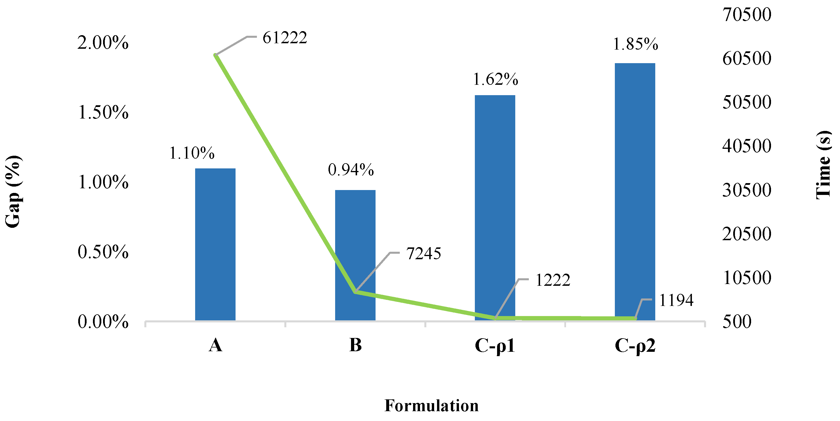
Ten scenarios were used to consider the uncertainty associated to wind production within the IEEE-RTS-96 test case, which were taken from Pandzic et al. [30]. Figure 2 compares the gap (%) (blue bars) and running time (s) (green line), taken to solve the SSCUC model for each formulation on the server. As shown by Ordoudis et al. [36], PHA is a promising algorithm with great potential to efficiently address the stochastic unit commitment problem in large-scale power systems as the number of scenarios increases.

Figure 2 shows that Formulation A takes a (large) computing time of $61,222$ s (approximately 17 h) to reach an optimality gap of $1.1$% with an objective function of $1.1110$ MUS$. Meanwhile, the performance of Formulation B is notably better; it took only 7245 s (approximately 2 h) to find a solution with an optimality gap of $0.94$% (which corresponds to an objective function of $1.1109$ MUS$). This is $8.5$ times faster with respect to the running time of Formulation A for a solution of even better quality. This first result illustrates that the inclusion of the $N-1$ cut-adding method proposed by Marín-Cano et al. [14] generates a more compact SSCUC model. Additionally, considering explicitly single contingencies for all 118 lines generates 3.3 million $N-1$ security constraints (in Formulation A). By contrast, the $N-1$ cut-adding method of Formulation C generated only 0.116 million binding security constraints defining the feasible region of the SSCUC problem. As a result, the cut-adding method embedded in PHA reduces the size of the model (of Formulation A) by 99.6% (by ignoring unnecessary security constraints within this model). As a consequence, the comparison of Formulations A and C (with ${\rho }_1$ and ${\rho }_2$) shows that the latter formulation achieves results of comparable quality in much faster running times. Even though the solutions reached by Formulation C have slightly greater optimality gaps (compared to the other formulations), it reaches acceptable sub-optimal solutions (with a gap of 1.62% for Formulation C-${\rho }_1$ and 1.85% for Formulation C-${\rho }_2$) in roughly 1200 s (approximately 20 min). Remarkably, Formulation C (with ${\rho }_1$ or ${\rho }_2$) is on average 50 times faster than Formulation A, and it is six times faster than Formulation B.

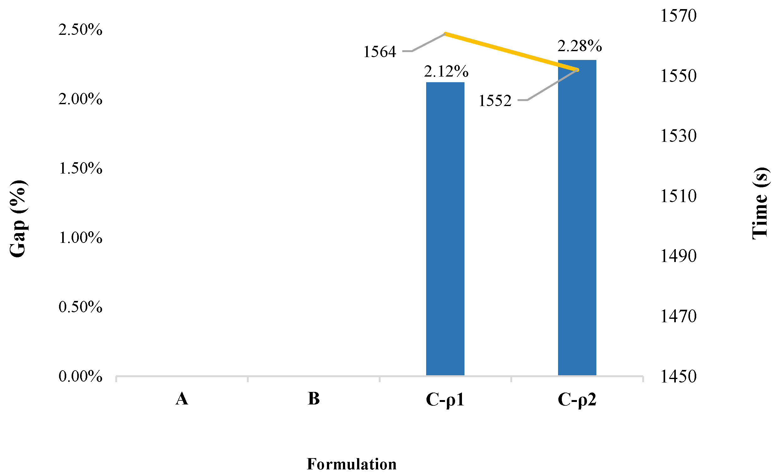
Figure 3 presents the performance of the proposed method in the test performed in the desktop, where blue bars are the optimality gap and yellow line is the running time taken by each formulation. This figure depicts clearly the value of the solution strategy presented in this paper. First, for Formulations A and B, no results were obtained, because a (standard) desktop computer does not have the computational resources required by these formulations. On the other hand, Formulation C (in both variants of the penalty factor update ${\rho }_1$ and ${\rho }_2$) obtained solutions with optimality gaps of around 2%. For example, Formulation C-${\rho }_1$ managed to obtain a gap of 2.12% (with a solution of 1.1223 MUS$) in a running time of 1564 s (26.1 min), whereas Formulation C-${\rho }_2$ reached a gap of $2.28$% in 1552 s ($25.8$ min). Notably, the results of both variants of Formulation C on the server (see Figure 2) and on the desktop computers (see Figure 3) are comparable in terms of both solution quality and running time. This, once again, shows the contribution of our novel strategy when it comes to obtaining high-quality solutions in short times, even when using computing resources of limited capacity.

On the other hand, Formulation C was unable to get solutions with gaps below 1% on the server (see Figure 2), as well as to get gaps below 2%, on the desktop computer (see Figure 3). This behavior is due to the fact that the $N-1$ SSCUC problem is an MIP problem with high dimensionality and PHA is a method that guarantees convergence and optimality only for convex problems. Therefore, some authors (e.g., Guo et al. [41]) have proposed integrating PHA with dual decomposition to have exact solutions for stochastic mixed-integer programming problems. However, Formulation C offers a good trade-off between the degree of suboptimality of the solution and the elapsed running time. The choice of the penalty factor updating strategies (Formulation C-${\rho }_1$ or Formulation C-${\rho }_2$) offers an additional control parameter, since the better is the quality of the solution (with Formulation C-${\rho }_1$) the longer is the running time. As a reference, detailed results of the experiments presented in this section are given in Appendix B.

5. Expansion Transmission Indices

In addition to establishing the safe operation of the system, an added value of the $N-1$ outage addition method proposed by Marín-Cano et al. [14] is the identification of the most severe line faults and vulnerable lines under contingency analysis. This additional information serves as indicative signals of needed expansion of the transmission system. These indices are computed considering the number of overloads and most severe outage of the network in scenario $\xi$ (i.e., $SC{R}_{l,k,t}\left(\xi \right))$.

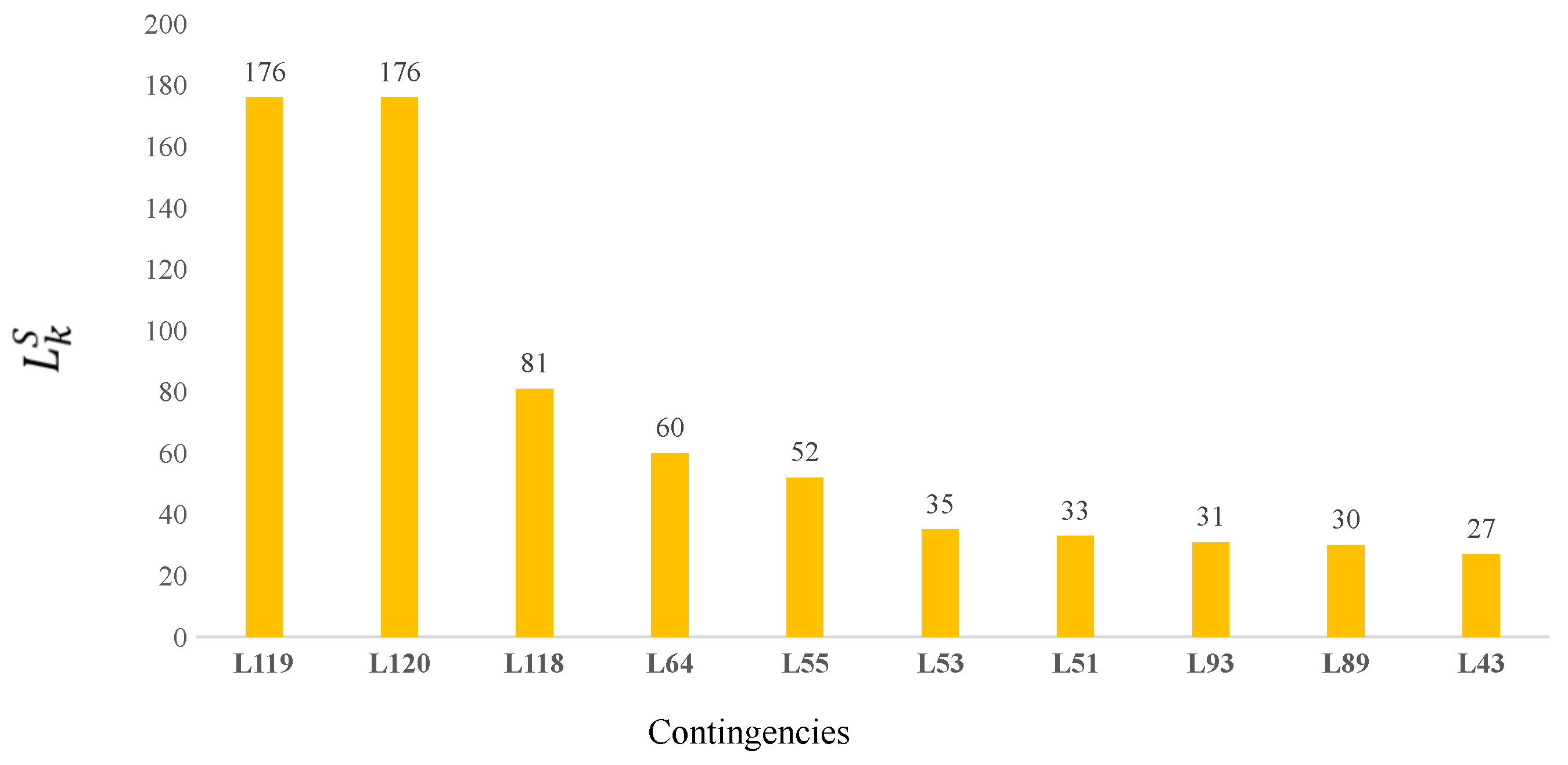
The most severe line failures are those whose contingency generates the greatest amount of overloads on other lines l. Index $L_k^S$ estimates the expected value of the number of lines l affected by contingency k, and it is obtained by rounding the weighted sum of the parameter $SC{R}_{l,k,t}\left(\xi \right)$ over the sets of time periods t, contingencies l and scenarios $\xi$. Briefly, $L_k^S$ indicates which line contingencies are the most severe, generating the greatest number of overloads on other lines.

$$L_k^S=\left[\sum _{t,l,\xi }{p}_{\xi }·SC{R}_{l,k,t}\left(\xi \right)\right],\forall k$$

(32)

As an example, Figure 4 shows the most severe line faults that cause the greatest overload impact on the system, according to parameter $L_k^S$. Outages of lines L119, L120, L118 and L64 (highlighted in orange in Figure 1) would generate, respectively, 176, 176, 81 and 60 thermal overloads in the transmission lines that remain in operation on the system.

Index $L_l^V$, estimates the expected value of the number of times that line l is overloaded when the contingency analysis is performed. This index show how vulnerable a line is when other lines are out of service. That is, $L_l^V$ indicates the number of overloads that a line experiences when transmission contingencies are produced in the system. This parameter is calculated by rounding the weighted sum of $SC{R}_{l,k,t}\left(\xi \right)$ over the sets of time periods t, contingencies k and scenarios $\xi$.

$$L_l^V=\left[\sum _{t,k,\xi }{p}_{\xi }·SC{R}_{l,k,t}\left(\xi \right)\right],\forall l$$

(33)

Figure 5 shows the most vulnerable lines of the IEEE-RTS-96 test system based on Index $L_l^V$. In this system, the lines with the highest number of overloads for different $N-1$ contingencies are L11, L118, L12 and L115 (highlighted in green in Figure 1), with 506, 349, 94 and 431 expected overloads over the time horizon and all scenarios, respectively.

Finally, the results of these indices suggest which lines to prioritize for the reinforcement of the transmission network through parallel circuits on some of the lines with the highest values of $L_l^V$ and $L_k^S$. This could guide short-term transmission expansion analyses aimed at reducing the risks of post-contingency overloads on other elements of the network. That, in turn, increases the security, reliability and operating margins of the power system to deal with an increasing demand in the short and medium terms.

6. Conclusions

This work presented a novel strategy to efficiently solve the Stochastic Security Constrained Unit Commitment (SSCUC) problem (coined as Formulation C through the paper). It combines Linear Sensitivity Factors (LSF), an efficient cut-adding method and the progressive hedging algorithm (PHA). The use of the cut-adding method reduces drastically (by 99%) the size of the problem by only including active $N-1$ security constraints in the model. Embedding (for the first time) this method into the PHA provides an effective and efficient solution approach, which is able to obtain solution of comparable quality but is 50 times faster than the extensive formulation (EF) of the SSCUC problem (Formulation A through the paper). Computational experiments also showed that the proposed solution strategy is stable to the choice of the updating procedure of the $\rho$ penalty factor, a key parameter for the successful convergence of the PHA. Additionally, the fine tuning of parameters $\alpha$ and $\beta$ depends on the problem characteristics (i.e., power system topology) and the need for high quality solutions of the SSCUC problem in short running times. The setting of these values allow the exploration of the trade-off between running time and solution quality. This characteristic of the proposed approach is valuable and can be exploited by the system operator when very short running times are needed.

Similarly, computational experiments on a (rather standard) desktop computer showed its value when it comes to obtain high quality solutions of the SSCUC problem with limited computational resources (where the EF or even the cut-adding method without PHA are not implementable). Additionally, as a side result of the proposed solution strategy, it is possible to identify the most affected (overloaded) lines before contingencies, as well as the most critical contingencies in the system. This is possible thanks to the values of two indices calculated with the information of the $N-1$ cuts added during the execution of the PHA iterative process. These two indices provide valuable information for decision-making during short- to medium-term transmission system expansion studies.

Although the PHA technique is more stable than other step-wise decomposition algorithms such as Benders decomposition, it is advisable to test the performance of the $N-1$ security constraint addition method with this type of technique. This suggest the integration of PHA and a promising decomposition method for Stochastic Mixed-Integer Programming: (i.e., Fenchel decomposition based on PHA), which has not yet been reported on the analysis of stochastic models for the operation of electrical power systems. Likewise, to further reduce the running time of the proposed approach, parallel versions of the solution strategy could be tested.

Finally, the method proposed in the paper can be extended to take into account other sources of uncertainty such as photovoltaic generation and demand, as well as batteries to hedge against them. For this, new constraints must be taken into account, such as the charging and discharging of batteries during the time horizon and the expected generation of the photovoltaic plants, among others.

References

1. Wang, C.; Fu, Y. Fully Parallel Stochastic Security-Constrained Unit Commitment. IEEE Trans. Power Syst. 2016, 31, 3561–3571. [Google Scholar] [CrossRef]
2. Tejada-Arango, D.A.; Sánchez-Martın, P.; Ramos, A. Security Constrained Unit Commitment Using Line Outage Distribution Factors. IEEE Trans. Power Syst. 2018, 33, 329–337. [Google Scholar] [CrossRef]
3. Ma, H.; Shahidehpour, S.M. Transmission-constrained unit commitment based on Benders decomposition. Int. J. Electr. Power Energy Syst. 1998, 20, 287–294. [Google Scholar] [CrossRef]
4. Shahidehpour, M.; Tinney, F.; Yong, F. Impact of Security on Power Systems Operation. Proc. IEEE 2005, 93. [Google Scholar] [CrossRef]
5. Fu, Y.; Shahidehpour, M.; Li, Z. AC contingency dispatch based on security-constrained unit commitment. IEEE Trans. Power Syst. 2006, 21, 897–908. [Google Scholar] [CrossRef]
6. Rahimi, S.; Niknam, T.; Fallahi, F. A New Approach Based on Benders Decomposition for Unit Commitment Problem. Word Appl. Sci. J. 2009, 6, 1665–1672. [Google Scholar]
7. Alemany, J.M.; Magnago, F.; Moitre, D. Benders Decomposition applied to Security Constrained Unit Commitment. IEEE Latin Am. Trans. 2013, 11, 421–425. [Google Scholar] [CrossRef]
8. Zhai, Q.; Guan, X.; Cheng, J.; Wu, H. Fast Identification of Inactive Security Constraints in SCUC Problems. IEEE Trans. Power Syst. 2010, 25, 1946–1954. [Google Scholar] [CrossRef]
9. Wu, H.; Guan, X.; Zhai, Q.; Ye, H. A Systematic Method for Constructing Feasible Solution to SCUC Problem With Analytical Feasibility Conditions. IEEE Trans. Power Syst. 2012, 27, 526–534. [Google Scholar] [CrossRef]
10. Ardakani, A.J.; Bouffard, F. Identification of umbrella constraints in DC-based security-constrained optimal power flow. In Proceedings of the 2014 IEEE PES General Meeting | Conference & Exposition, National Harbor, MD, USA, 27–31 July 2014; p. 1. [Google Scholar] [CrossRef]
11. Capitanescu, F.; Glavic, M.; Ernst, D.; Wehenkel, L. Contingency Filtering Techniques for Preventive Security-Constrained Optimal Power Flow. IEEE Trans. Power Syst. 2007, 22, 1690–1697. [Google Scholar] [CrossRef]
12. Wood, A.J.; Wollenberg, B.F.; Sheble, G.B. Power Generation, Operation, and Control, 3rd ed.; Wiley: Hoboken, NJ, USA, 2013. [Google Scholar]
13. Eslami, M.; Moghadam, H.A.; Zayandehroodi, H.; Ghadimi, N. A New Formulation to Reduce the Number of Variables and Constraints to Expedite SCUC in Bulky Power Systems. Proc. Natl. Acad. Sci. India Sec. A Phys. Sci. 2019, 89, 311–321. [Google Scholar] [CrossRef]
14. Marín-Cano, C.C.; Sierra-Aguilar, J.E.; López-Lezama, J.M.; Jaramillo-Duque, A.; Villa-Acevedo, W.M. Implementation of User Cuts and Linear Sensitivity Factors to Improve the Computational Performance of the Security-Constrained Unit Commitment Problem. Energies 2019, 12, 1399. [Google Scholar] [CrossRef] [Green Version]
15. Xavier, A.S.; Qiu, F.; Wang, F.; Thimmapuram, P.R. Transmission Constraint Filtering in Large-Scale Security-Constrained Unit Commitment. IEEE Trans. Power Syst. 2019, 34, 2457–2460. [Google Scholar] [CrossRef]
16. Van Ackooij, W.; Lopez, I.D.; Frangioni, A.; Lacalandra, F.; Tahanan, M. Large-scale unit commitment under uncertainty: An updated literature survey. Ann. Oper. Res. 2018, 271, 11–85. [Google Scholar] [CrossRef] [Green Version]
17. Wu, L.; Shahidehpour, M.; Li, Z. Comparison of Scenario-Based and Interval Optimization Approaches to Stochastic SCUC. IEEE Trans. Power Syst. 2012, 27, 913–921. [Google Scholar] [CrossRef]
18. Wu, L.; Shahidehpour, M.; Li, T. Stochastic Security-Constrained Unit Commitment. IEEE Trans. Power Syst. 2007, 22, 800–811. [Google Scholar] [CrossRef]
19. Wang, J.; Shahidehpour, M.; Li, Z. Security-Constrained Unit Commitment With Volatile Wind Power Generation. IEEE Trans. Power Syst. 2008, 23, 1319–1327. [Google Scholar] [CrossRef]
20. Hreinsson, K.; Vrakopoulou, M.; Andersson, G. Stochastic security constrained unit commitment and non-spinning reserve allocation with performance guarantees. Int. J. Electr. Power Energy Syst. 2015, 72, 109–115. [Google Scholar] [CrossRef]
21. Sundar, K.; Nagarajan, H.; Lubin, M.; Roald, L.; Misra, S.; Bent, R.; Bienstock, D. Unit commitment with N − 1 Security and wind uncertainty. In Proceedings of the 2016 Power Systems Computation Conference (PSCC), Genoa, Italy, 20–24 June 2016; pp. 1–7. [Google Scholar] [CrossRef] [Green Version]
22. Alizadeh-Mousavi, O.; Nick, M. Stochastic Security Constrained Unit Commitment with variable-speed pumped-storage Hydropower Plants. In Proceedings of the 2016 Power Systems Computation Conference (PSCC), Genoa, Italy, 20–24 June 2016; pp. 1–7. [Google Scholar] [CrossRef]
23. Park, H.; Jin, Y.G.; Park, J.K. Stochastic security-constrained unit commitment with wind power generation based on dynamic line rating. Int. J. Electr. Power Energy Syst. 2018, 102, 211–222. [Google Scholar] [CrossRef]
24. Zheng, Q.P.; Wang, J.; Liu, A.L. Stochastic Optimization for Unit Commitment: A Review. IEEE Trans. Power Syst. 2015, 30, 1913–1924. [Google Scholar] [CrossRef]
25. Yang, N.; Ye, D.; Zhou, Z.; Huang, Y.; Dong, B. Research on Solving Method of Security Constrained Unit Commitment Based on Improved Stochastic Constrained Ordinal Optimization. In Proceedings of the 2018 3rd International Conference on Intelligent Green Building and Smart Grid (IGBSG), Yi-Lan, Taiwan, 22–25 April 2018; pp. 1–4. [Google Scholar] [CrossRef]
26. Wu, H.; Shahidehpour, M. Stochastic SCUC Solution With Variable Wind Energy Using Constrained Ordinal Optimization. IEEE Trans. Sustain. Energy 2014, 5, 379–388. [Google Scholar] [CrossRef]
27. Watson, J.P.; Woodruff, D.L. Progressive hedging innovations for a class of stochastic mixed-integer resource allocation problems. Comput. Manag. Sci. 2011, 8, 355–370. [Google Scholar] [CrossRef]
28. Gade, D.; Hackebeil, G.; Ryan, S.M.; Watson, J.P.; Wets, R.J.B.; Woodruff, D.L. Obtaining lower bounds from the progressive hedging algorithm for stochastic mixed-integer programs. Math. Program. 2016, 157, 47–67. [Google Scholar] [CrossRef] [Green Version]
29. Pandžić, H.; Qiu, T.; Kirschen, D.S. Comparison of state-of-the-art transmission constrained unit commitment formulations. In Proceedings of the 2013 IEEE Power & Energy Society General Meeting, Vancouver, BC, Canada, 21–25 July 2013; pp. 1–5. [Google Scholar] [CrossRef]
30. Pandzic, H.; Dvorkin, Y.; Qiu, T.; Wang, Y.; Kirschen, D. Unit Commitment under Uncertainty—GAMS Models; Library of the Renewable Energy Analysis Lab (REAL), University of Washington: Seattle, WA, USA, 2017; Available online: https://www2.ee.washington.edu/research/real/gams_code.html (accessed on 20 July 2018).
31. IBM®-IBM Knowledge Center. Differences between User Cuts and Lazy Constraints. 2014. Available online: https://www.ibm.com/support/knowledgecenter/SSSA5P12.7.0/ilog.odms.cplex.help/CPLEX/UsrMan/topics/progradv/usrcutlazyconstr/02defn.html (accessed on 15 February 2019).
32. Ryan, S.; Wets, R.B.; Woodruff, D.; Silva-Monroy, C.; Watson, J.P. Toward scalable, parallel progressive hedging for stochastic unit commitment. In Proceedings of the 2013 IEEE Power Energy Society General Meeting, Vancouver, BC, Canada, 21–25 July 2013; pp. 1–5. [Google Scholar]
33. Rockafellar, R.T.; Wets, R.J.B. Scenarios and Policy Aggregation in Optimization Under Uncertainty. Math. Oper. Res. 1991, 16, 119–147. [Google Scholar] [CrossRef]
34. Gonçalves, R.E.C.; Finardi, E.C.; Silva, E.L.D. Applying different decomposition schemes using the progressive hedging algorithm to the operation planning problem of a hydrothermal system. Electr. Power Syst. Res. 2012, 83, 19–27. [Google Scholar] [CrossRef]
35. Li, C.; Zhang, M.; Hedman, K.W. N − 1 Reliable Unit Commitment via Progressive Hedging. J. Energy Eng. 2015, 141, B4014004. [Google Scholar] [CrossRef]
36. Ordoudis, C.; Pinson, P.; Zugno, M.; Morales, J.M. Stochastic unit commitment via Progressive Hedging—Extensive analysis of solution methods. In Proceedings of the 2015 IEEE Eindhoven PowerTech, Eindhoven, The Netherlands, 29 June–2 July 2015; pp. 1–6. [Google Scholar] [CrossRef]
37. Gil, E.; Araya, J. Short-term Hydrothermal Generation Scheduling Using a Parallelized Stochastic Mixed-integer Linear Programming Algorithm. Energy Procedia 2016, 87, 77–84. [Google Scholar] [CrossRef] [Green Version]
38. Dos Santos, M.L.L.; da Silva, E.L.; Finardi, E.C.; Gonçalves, R.E.C. Practical aspects in solving the medium-term operation planning problem of hydrothermal power systems by using the progressive hedging method. Int. J. Electr. Power Energy Syst. 2009, 31, 546–552. [Google Scholar] [CrossRef]
39. Mulvey, J.M.; Vladimirou, H. Applying the progressive hedging algorithm to stochastic generalized networks. Ann. Oper. Res. 1991, 31, 399–424. [Google Scholar] [CrossRef]
40. Zehtabian, S.; Bastin, F. Penalty Parameter Update Strategies in Progressive Hedging Algorithm; CIRRELT: Montreal, QC, Canada, 2016. [Google Scholar]
41. Guo, G.; Hackebeil, G.; Ryan, S.M.; Watson, J.P.; Woodruff, D.L. Integration of progressive hedging and dual decomposition in stochastic integer programs. Oper. Res. Lett. 2015, 43, 311–316. [Google Scholar] [CrossRef] [Green Version]
Figure 1. Test system under study (IEEE RTS-96).
Energies 13 03777 g001
Figure 2. Optimality gap (%) and running time (s) for the different formulations on the server.
Energies 13 03777 g002
Figure 3. Optimality gap (%) vs. running time (s) for the different formulations on the desktop.
Energies 13 03777 g003
Figure 4. L k S : The average number of lines l affected by contingency k.
Energies 13 03777 g004
Figure 5. L l V : The average number of times that line l is overloaded, given a k single contingency.
Energies 13 03777 g005