1. Introduction
Offshore-located wind-turbines are always clustered in wind farms to limit overall installation and maintenance expenses. Today, the potential offshore market is also the main driver for the development of large wind-turbines. As shown in
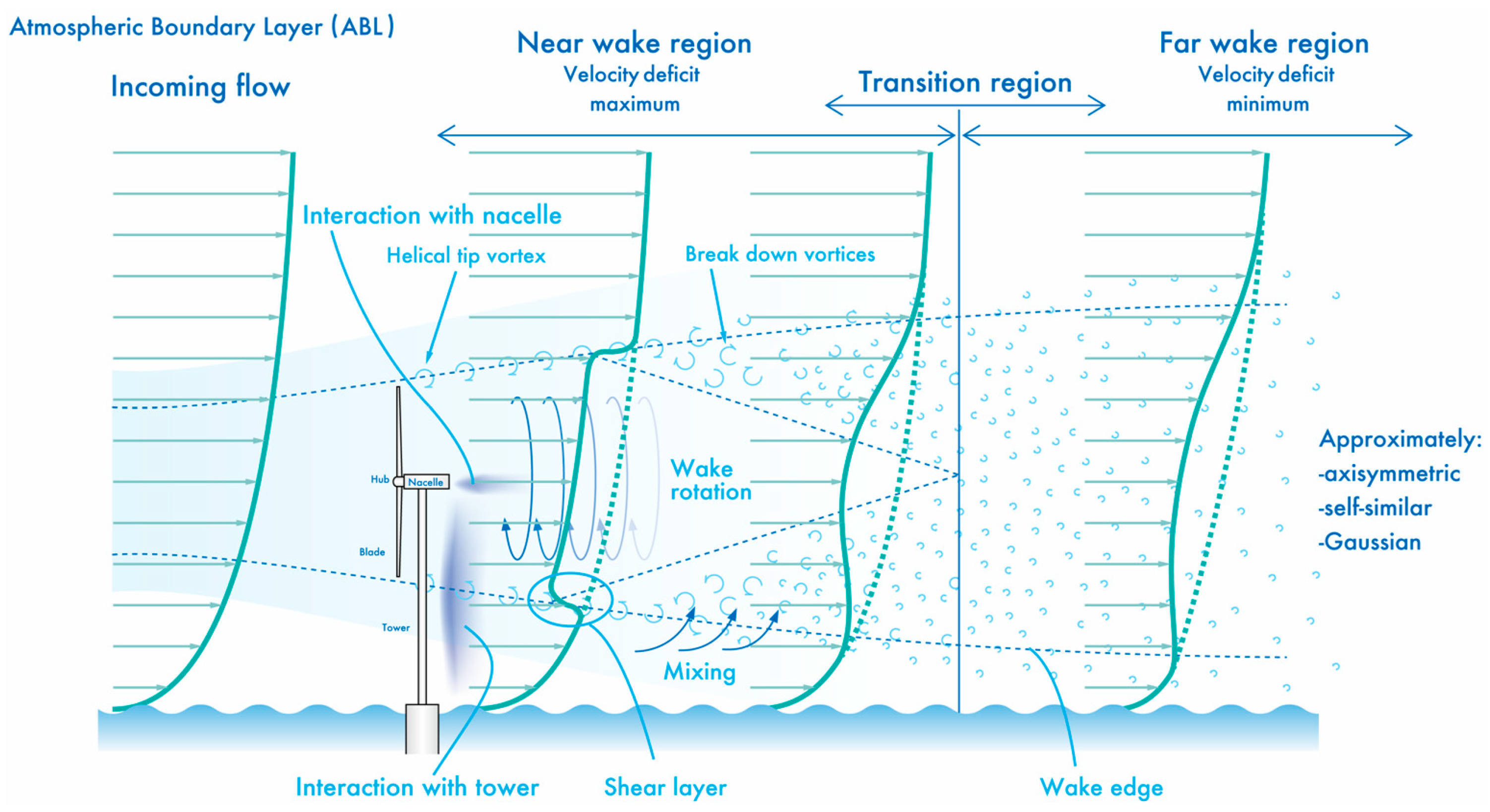
Figure 1, with the rotation of the blade of the wind-turbine, a region of wind-velocity deficit with temporal and spatial variations is formed downstream of the wind-turbine. This flow phenomenon is called wind-turbine wake. Wind-turbines in offshore wind farms operating in downwind wake flow are subjected to two main problems. One is decreased energy production due to the wind-velocity deficit, and the other is increased fatigue loading due to the added turbulence intensity generated by the upwind turbine. The mutual interference of wind-turbine wake, which is a strongly nonlinear flow phenomenon, occurs especially in large offshore wind farms consisting of multiple wind-turbine groups. The mutual interference of wind-turbine wakes is an essential and inherent problem in offshore wind farms. Therefore, in order to improve the power efficiency and lifetime of a wind-turbine, an accurate understanding of wake effects due to the mutual interaction between the wakes of the wind-turbines is extremely important [
1,
2,
3,
4,
5,
6,
7,
8,
9,
10,
11,
12,
13,
14].
For accurate evaluation of wind-turbine wake flows, field measurements and wind-tunnel experiments using a scale model are currently problematic. Therefore, engineering wake models (empirical/analytical wake models represented by Jensen [
15]/Katic [
16]), computational fluid dynamics (CFD) with the wake model using an actuator disk (AD) model [
17], the actuator disk model with rotation (ADM-R) [
18], actuator line (AL) model [
19], actuator surface (AS) model [
20], and numerical investigations based on fully resolved geometries combined with CFD simulations [
21] are generally used.
In this study, we focused on the incoming flow conditions of a wind-turbine (two sheared and one uniform inflow) and examined the effects of inflow shear on the wake characteristics of wind-turbines over flat terrain. The effect of mean shear in conjunction with other effects (atmospheric stratification or turbulence intensity) on wind-turbine-wake recovery has been investigated. The effect of shear alone on wind-turbine wake recovery has not been investigated. For this purpose, the approach of CFD by large-eddy simulation (LES) was adopted. In this study, we constructed an in-house LES solver called RIAM-COMPACT [
22,
23,
24,
25,
26,
27] based on the Cartesian staggered grid. In this study, we adopted the AL model for the rotation of wind-turbine blades as a method in which numerical simulations for multiple wind-turbines are relatively easy.
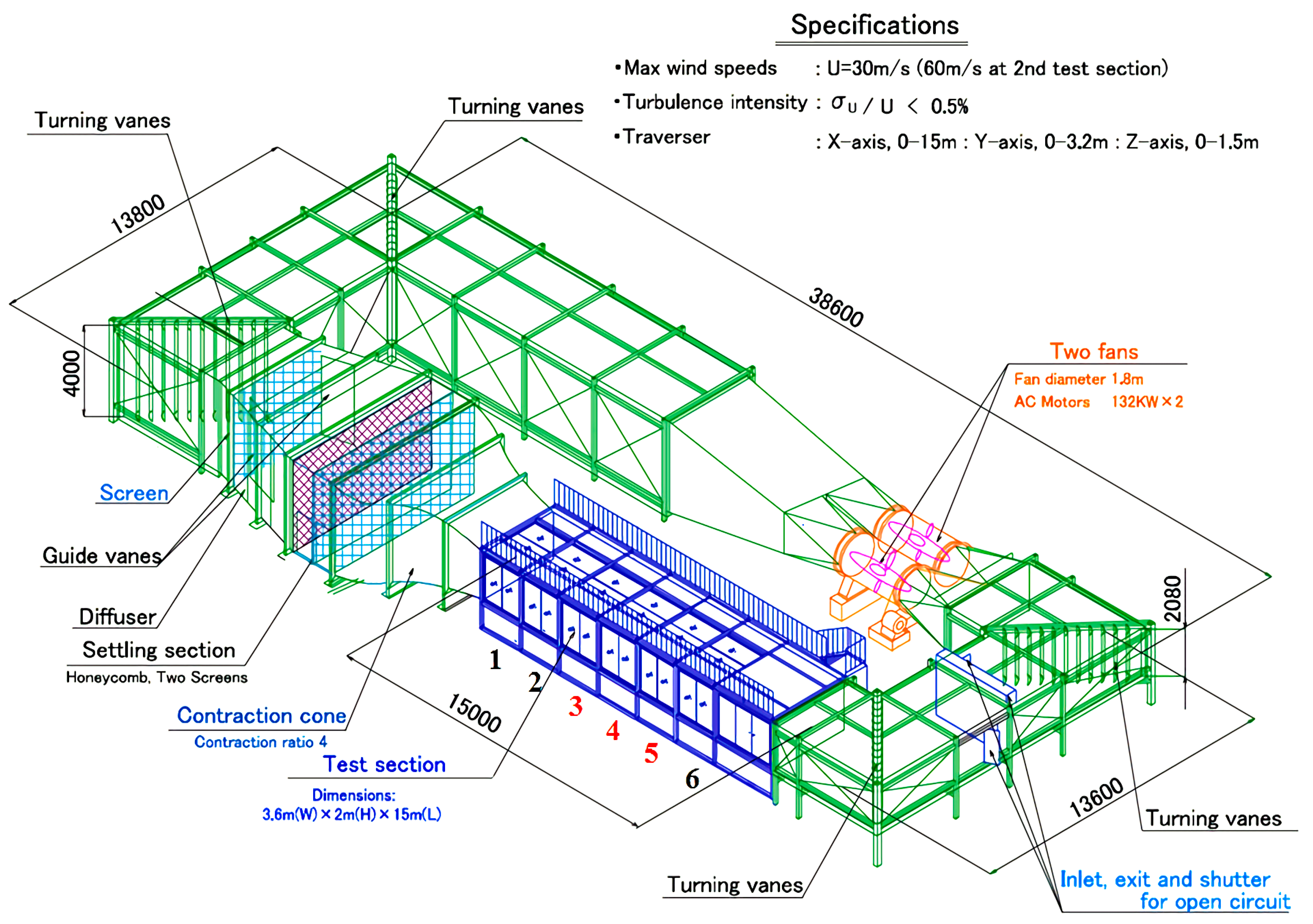
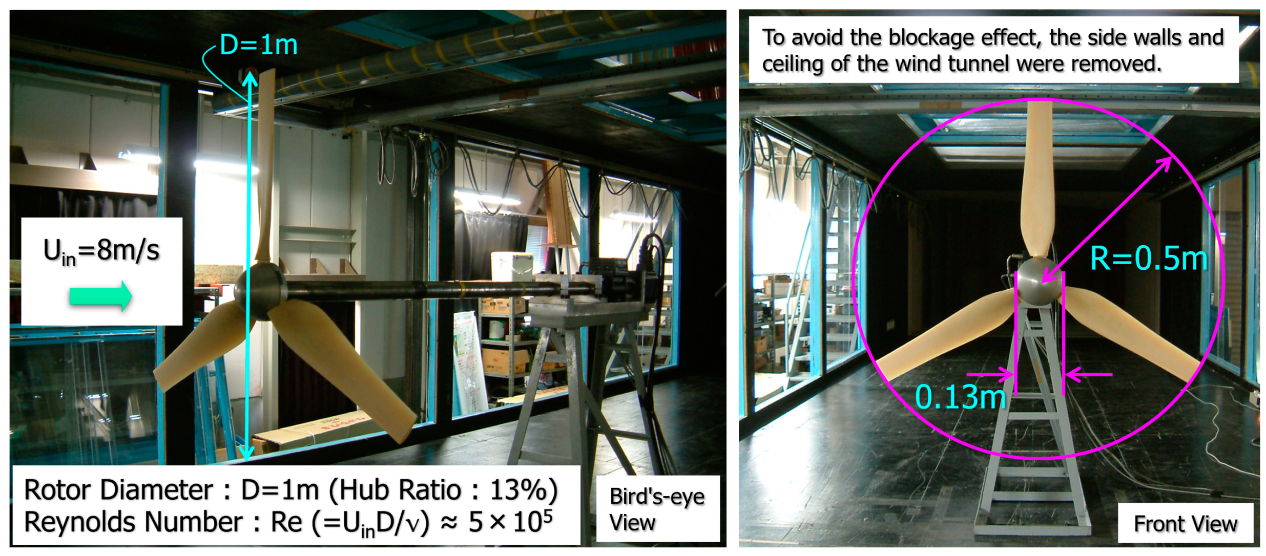
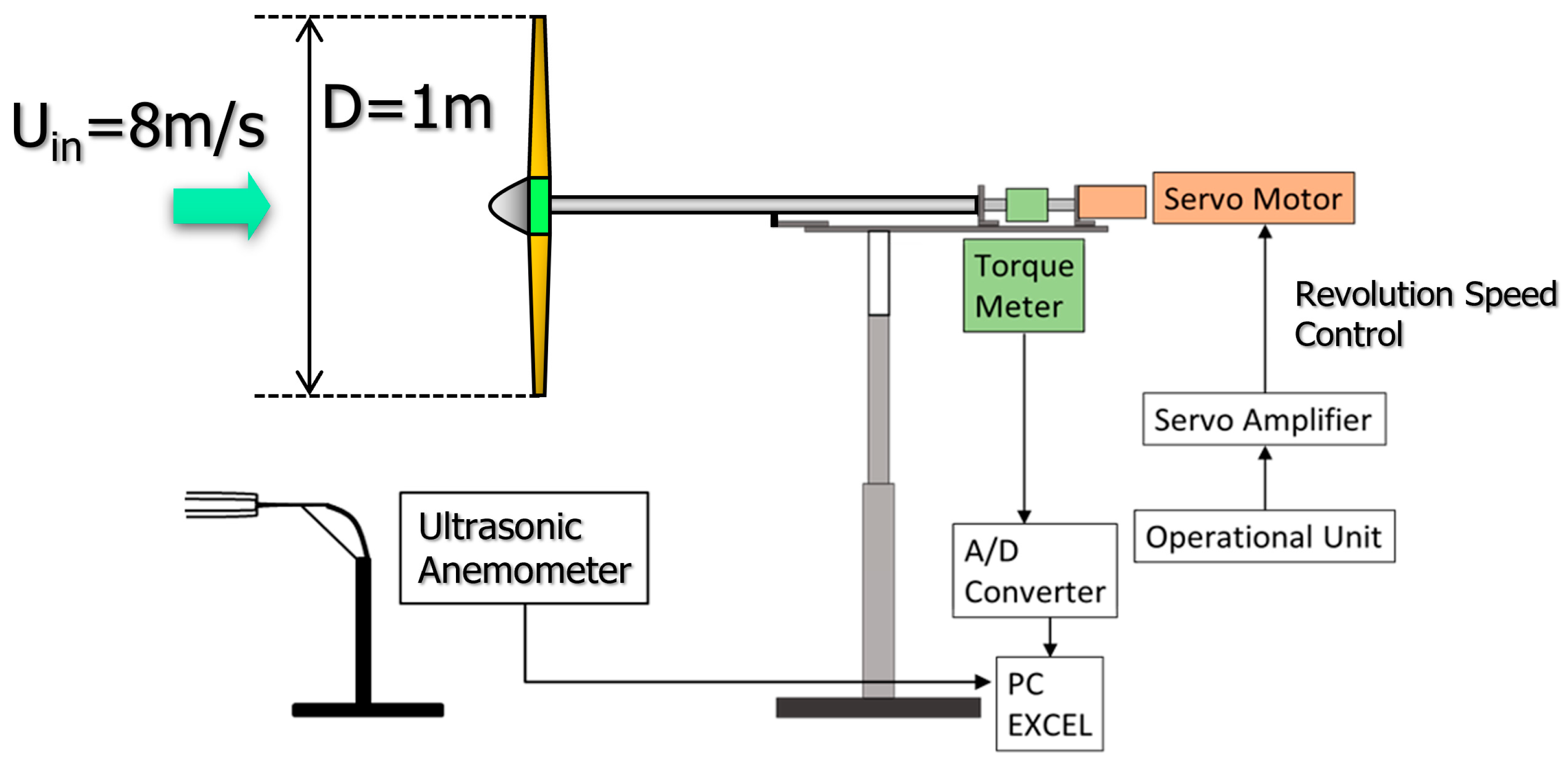
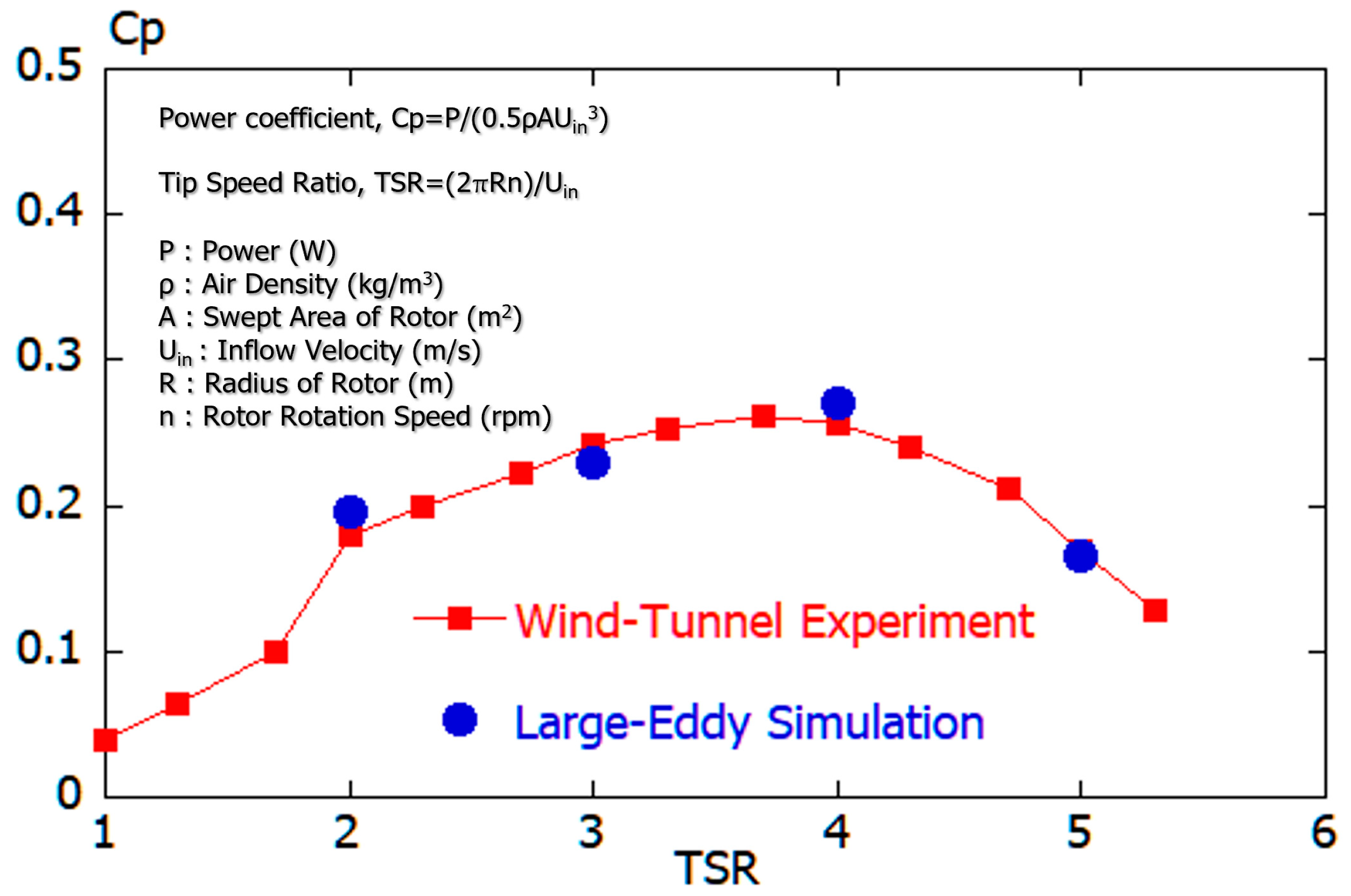
The scope of the present study is to understand the wake characteristics of wind-turbines, under various inflow shears. First, in order to verify the prediction accuracy of the in-house LES solver based on a Cartesian staggered grid, RIAM-COMPACT, we conducted a wind-tunnel experiment using a wind-turbine scale model, and compared the numerical and experiment results. Next, with the developed in-house LES solver, flow past the entire wind-turbine (isolated wind-turbine), including the nacelle and the tower, was simulated for a tip speed ratio of 4, the optimal tip-speed ratio (TSR). On the basis of the obtained results, we numerically investigated the effects of inflow shear on the wake characteristics of wind-turbines over a flat terrain.
3. Effects of Inflow Shear on Wake Characteristics of Wind-Turbines over Flat Terrain
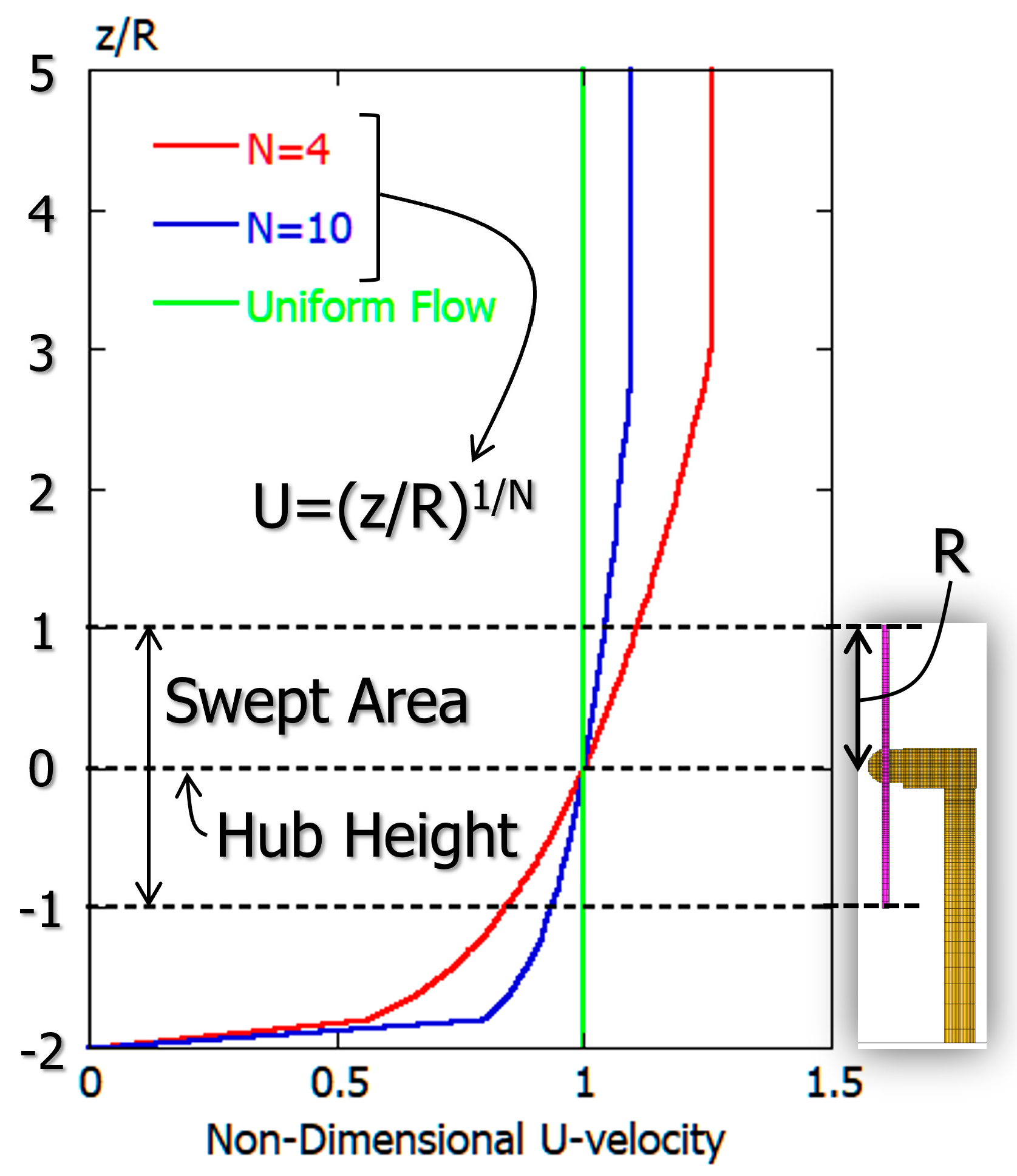
Here, as shown in
Figure 12 and
Figure 13, various inflow shears were assumed at the inflow boundary surface, and we conducted wind-turbine wake simulations installed on a flat terrain. On the basis of the obtained results, the effect of inflow shear on the flow characteristics in the wind-turbine wake region was considered. Similar to the calculation shown in
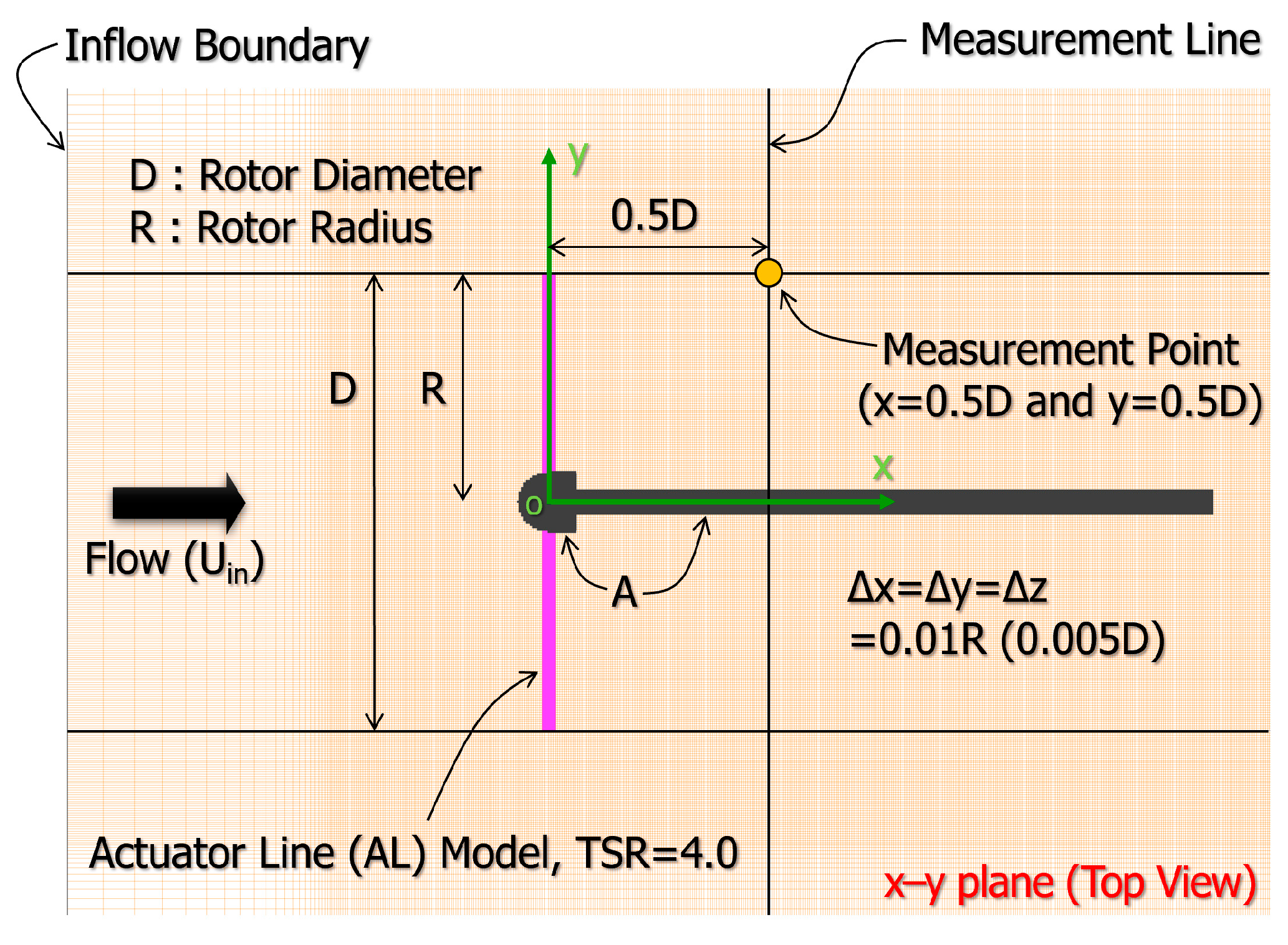
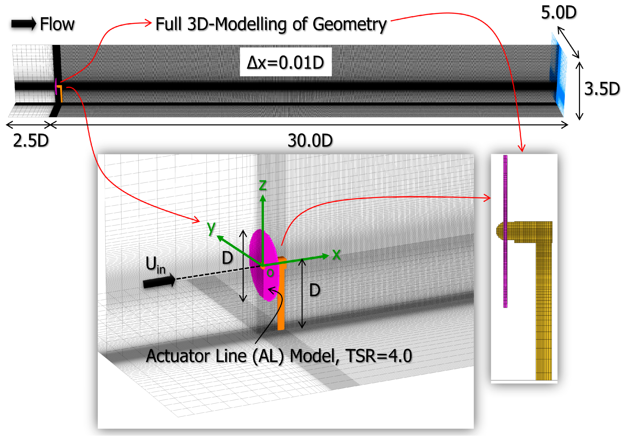
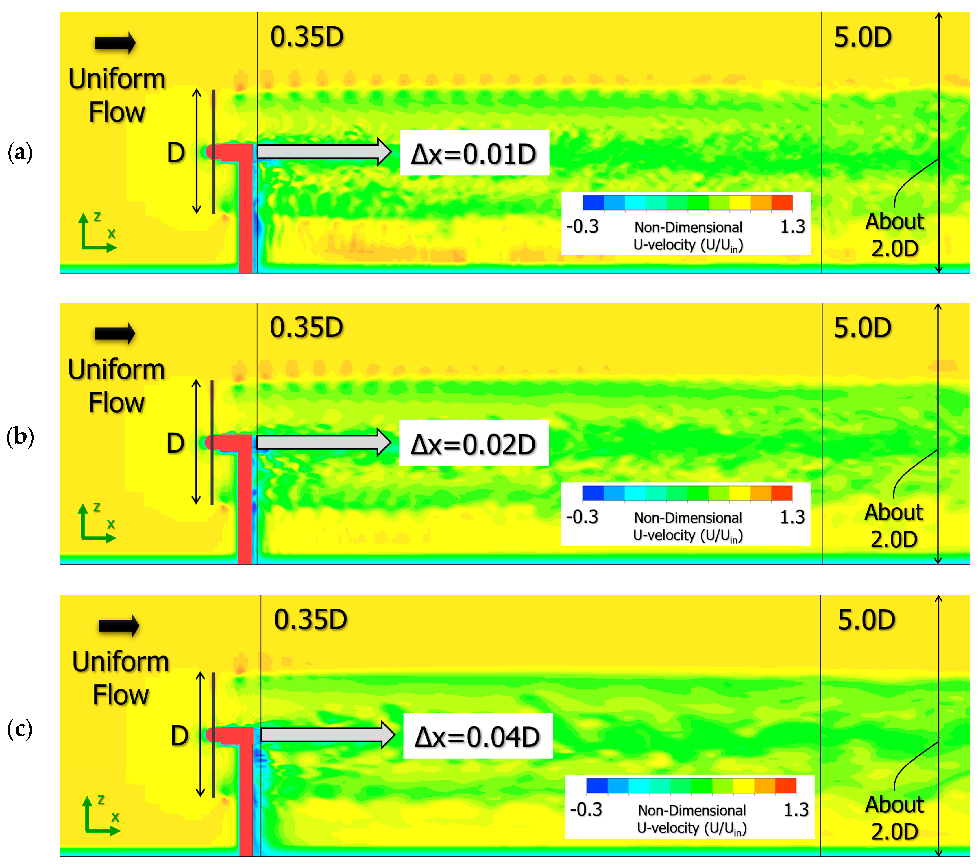
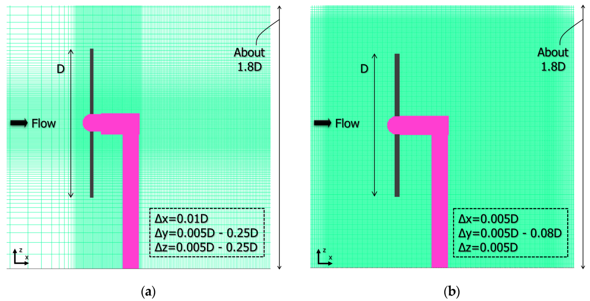
Section 2, the wind-turbine blades were rotated at the optimal TSR = 4.0, at which the power coefficient Cp showed the maximum value. In order to reproduce the shape of the nacelle and tower, the spatial grid resolution in the vicinity of the wind-turbine was set to Δx = Δy = Δz = 0.005 D (x+ = y+ = z+ < 10.0). Here, D is the diameter of the wind-turbine blade. In order to eliminate the influence of the spatial-grid resolution on the reproduction accuracy of the wind-turbine wake as much as possible, the spatial-grid resolutions in the x direction were all the same downstream of the wind-turbine, and Δx = 0.01 D. The total number of grid points in the entire computational domain was about 85 million (3075 (x) × 171 (y) × 161 (z)). In particular, we focused on reproducing the generation and collapse of tip vortex, and set the spatial resolution in the streamwise direction (see
Appendix C). The boundary conditions of velocity at the other boundaries except for the inflow boundary surface were as shown below. Slip conditions were imposed on the upper- and lateral-boundary surfaces. No-slip conditions were applied on the ground, and convection-type outflow conditions were applied on the outflow boundary surface. Boundary conditions for pressure were Neumann conditions on all boundary surfaces. Other conditions were the same as those in the calculation in
Section 2. The time step was Δt = 1 × 10
−3 R/U
in. In this calculation, the calculation domain in the x direction was very long, 30.0 D; thus, a long-term integration of t = 0 to 400 R/U
in was performed. Various turbulence statistics were calculated at t = 200 to 400 R/U
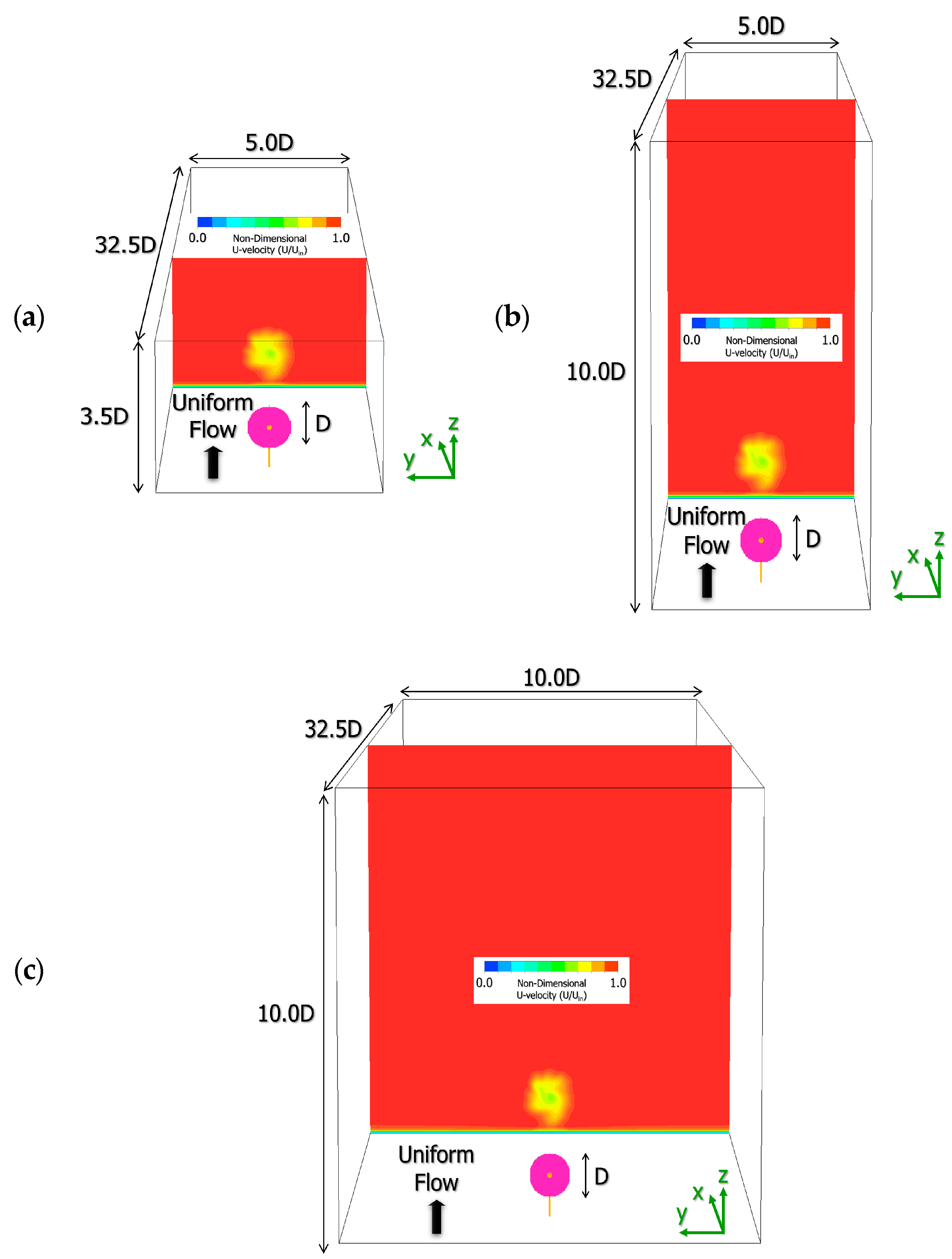
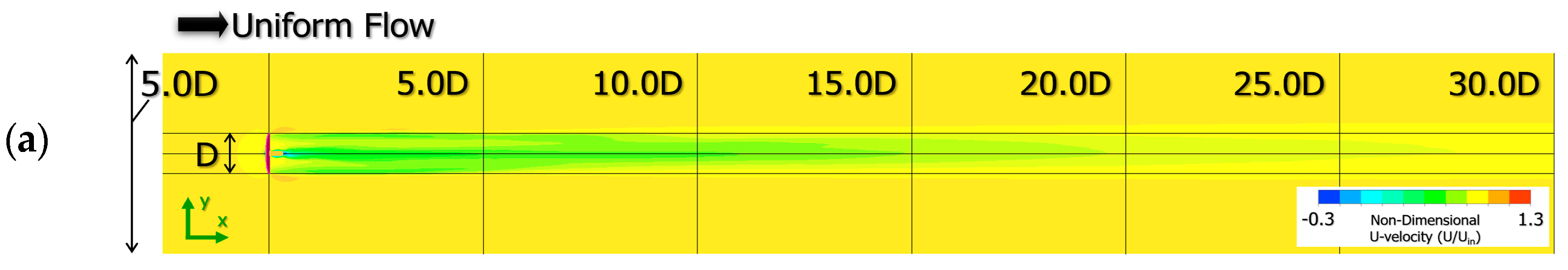
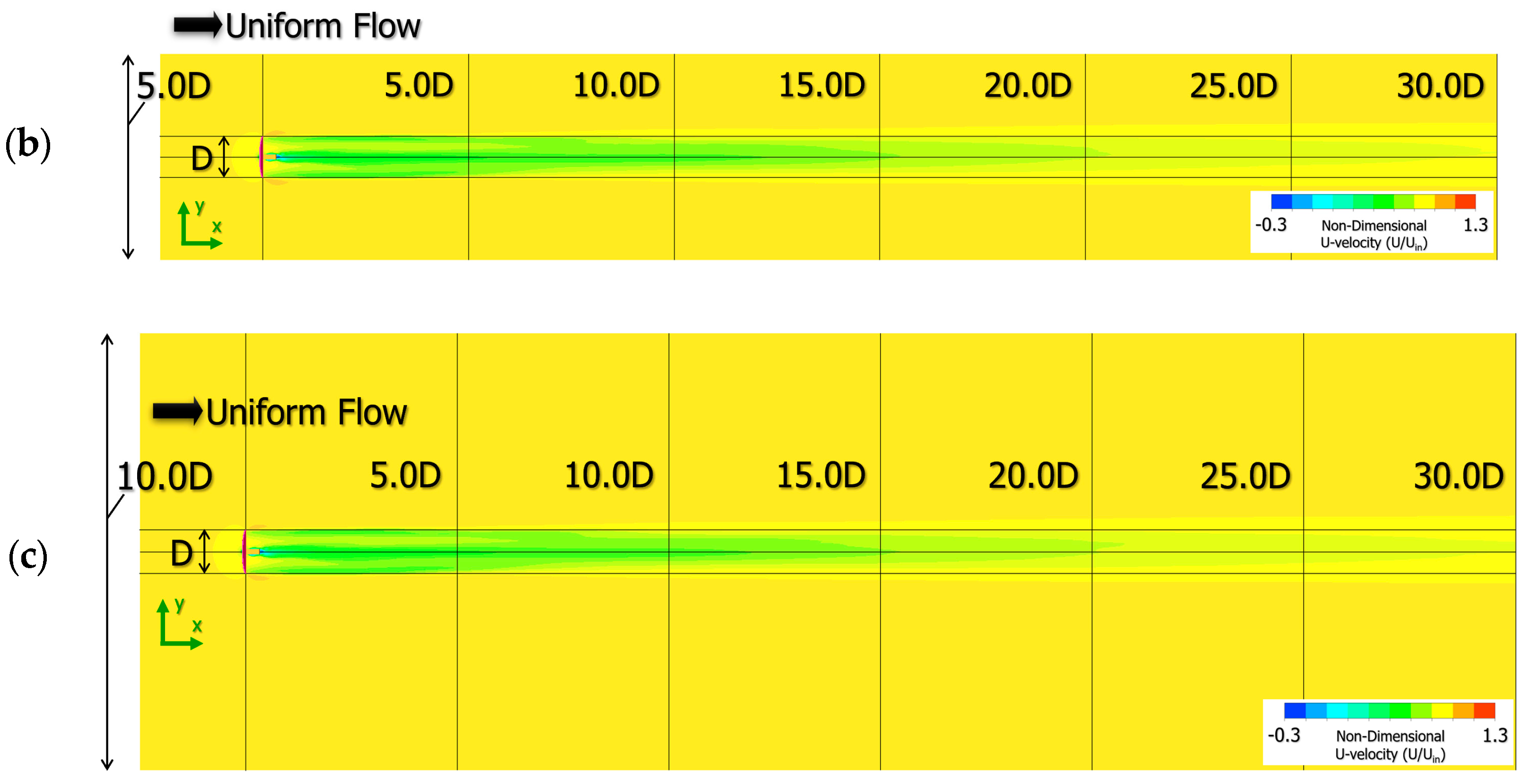
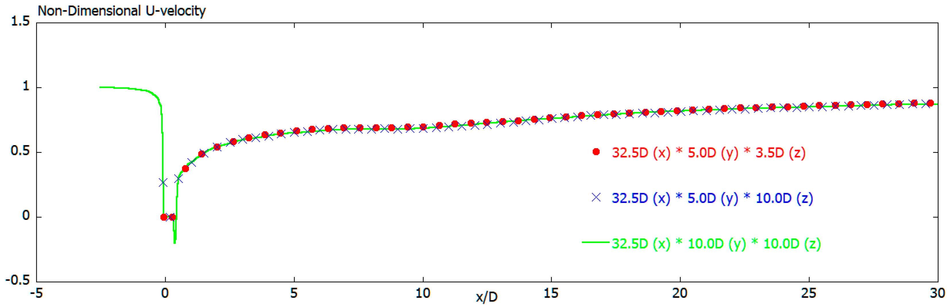
in. In this study, the some calculations were performed by changing the domain size, and its effect was also examined (see
Appendix B). The calculations in this study were performed using a new SX-Aurora TSUBASA vector supercomputer. The CPU time required for each calculation is about several days.
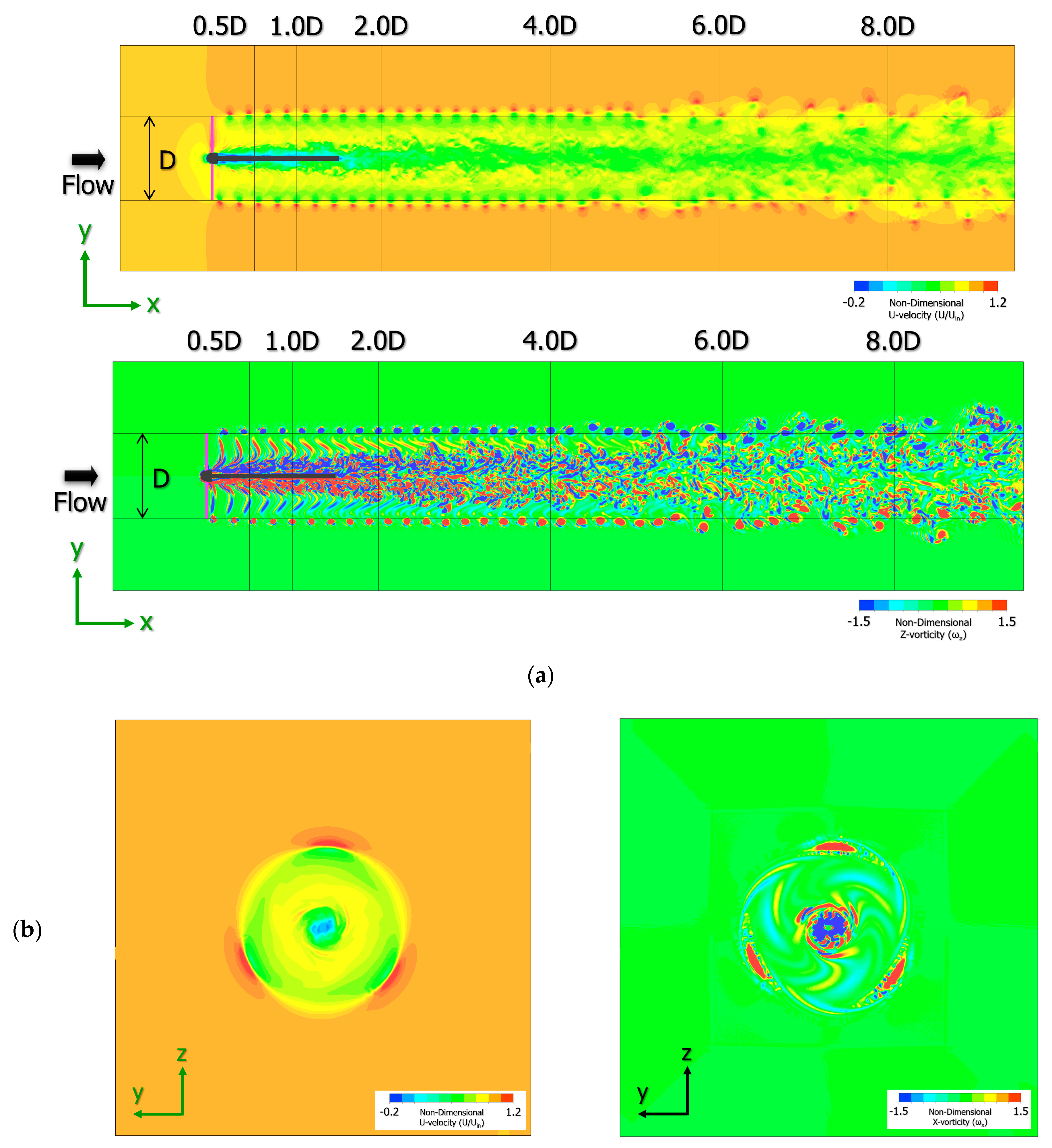
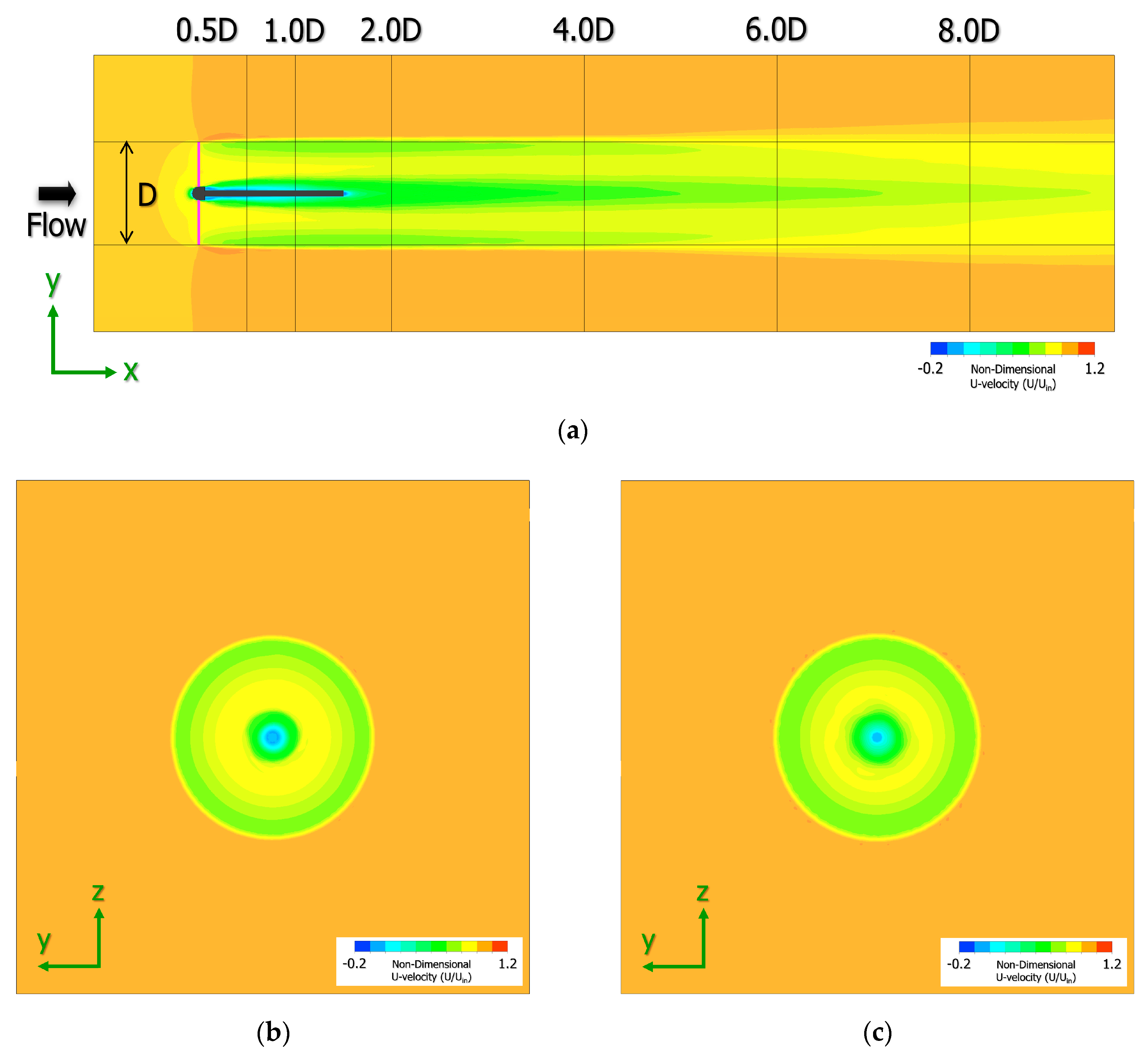
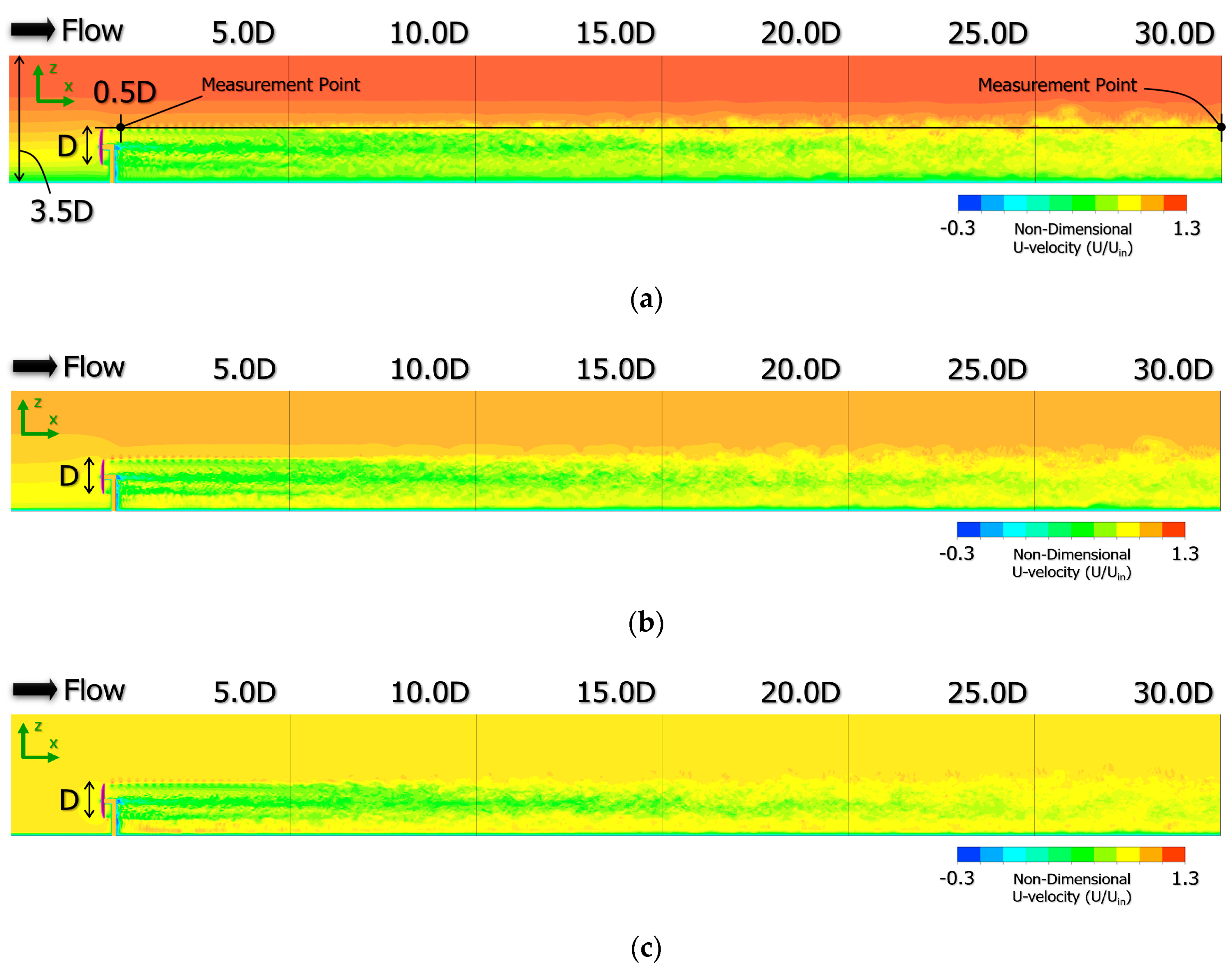
Figure 14 shows spatial distribution of instantaneous U-velocity in the mid-span plane (side view) at t = 400 R/U
in. In all cases of N = 4 shown in
Figure 14a, N = 10 shown in
Figure 14b, and uniform flow shown in
Figure 14c, periodic shedding of the tip vortex was clearly observed in the near-wake region of x = 5.0 D. In all cases, a vertical meandering motion of the wind-turbine wake occurred from around x = 6.0 D. After that, in the far-wake region where x = 10.0 D, the amount of change in vertical meandering motion was even larger. We can see the entrainment of ambient fluid into the wake-flow region. In other words, the rapid mixing and exchange of fluid volumes across the wake edge occurred.
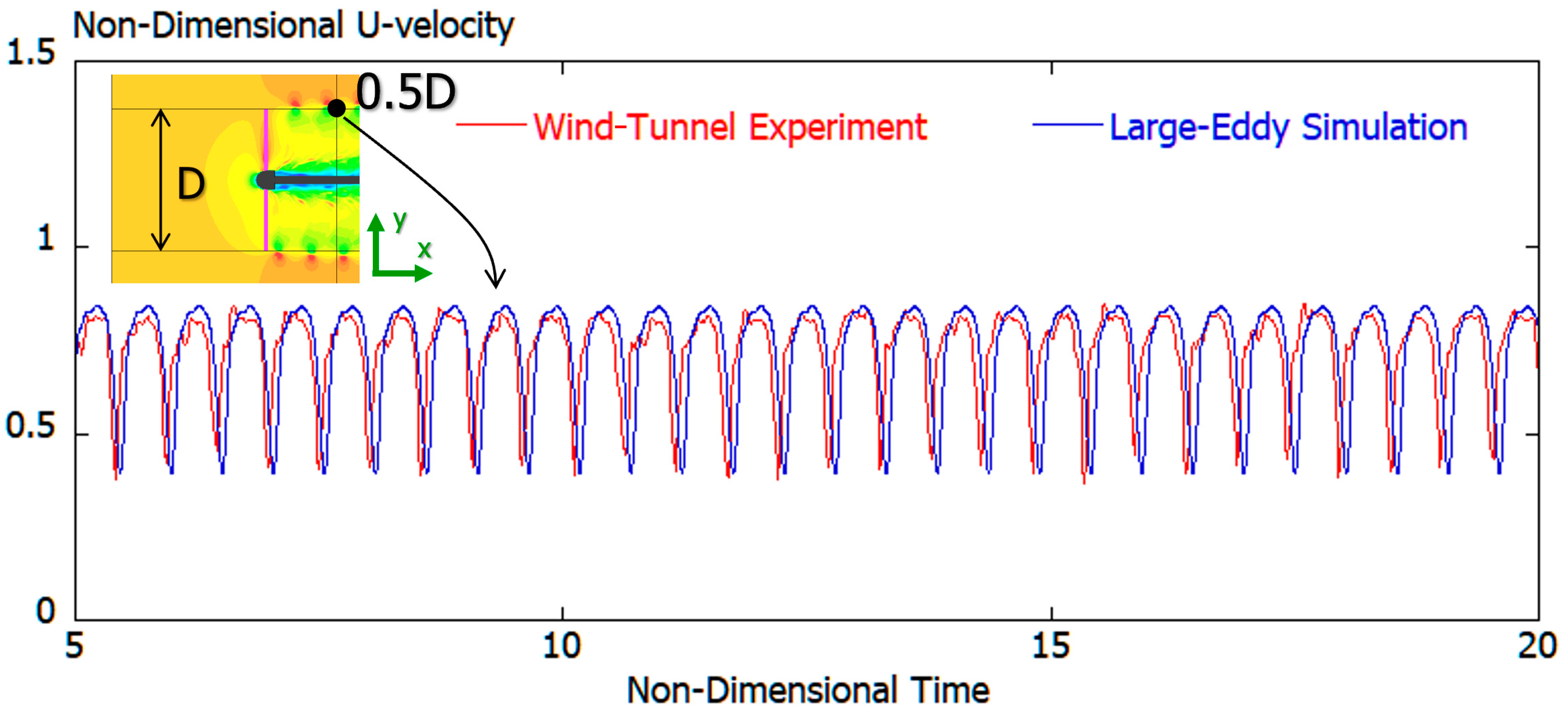
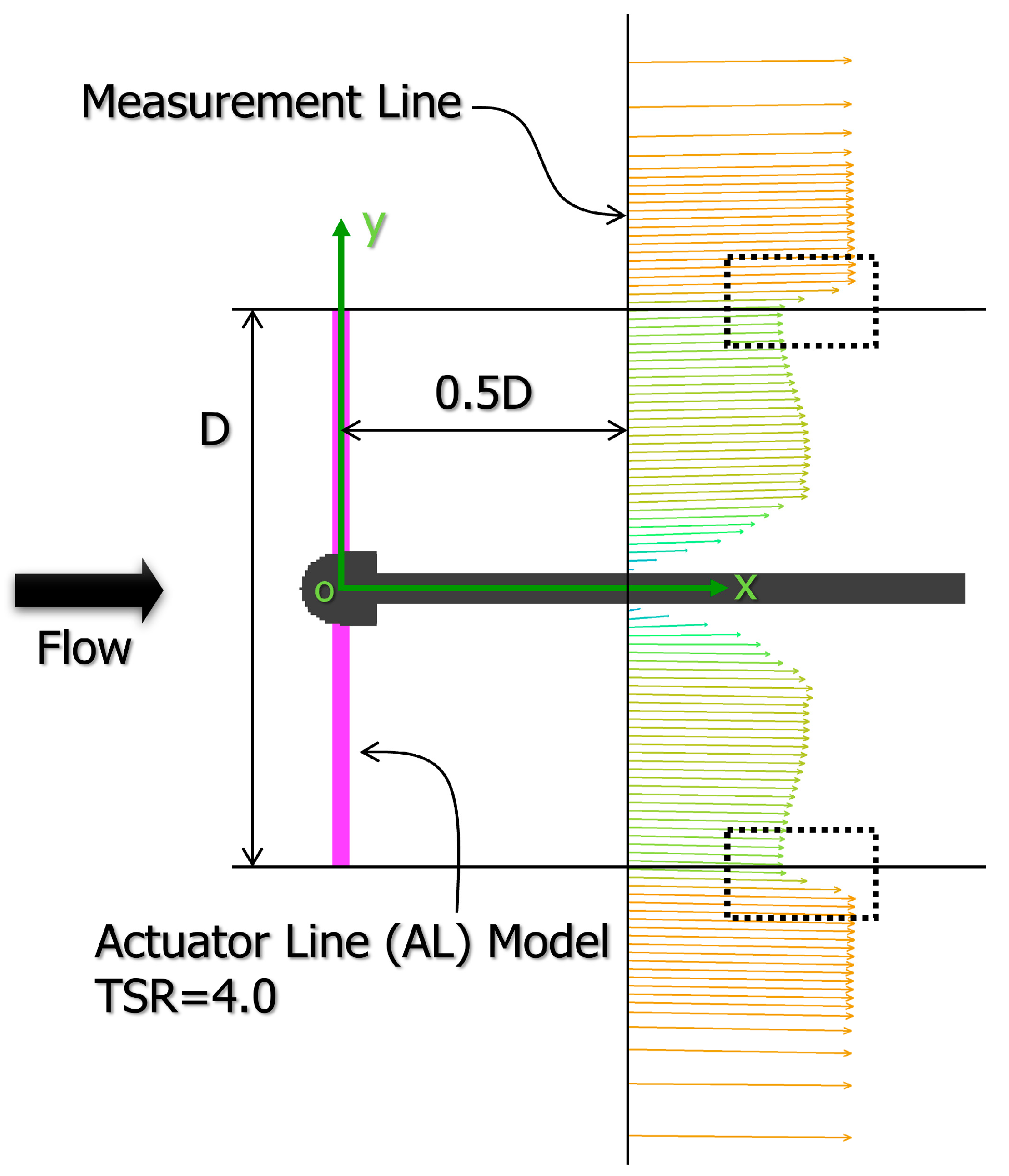
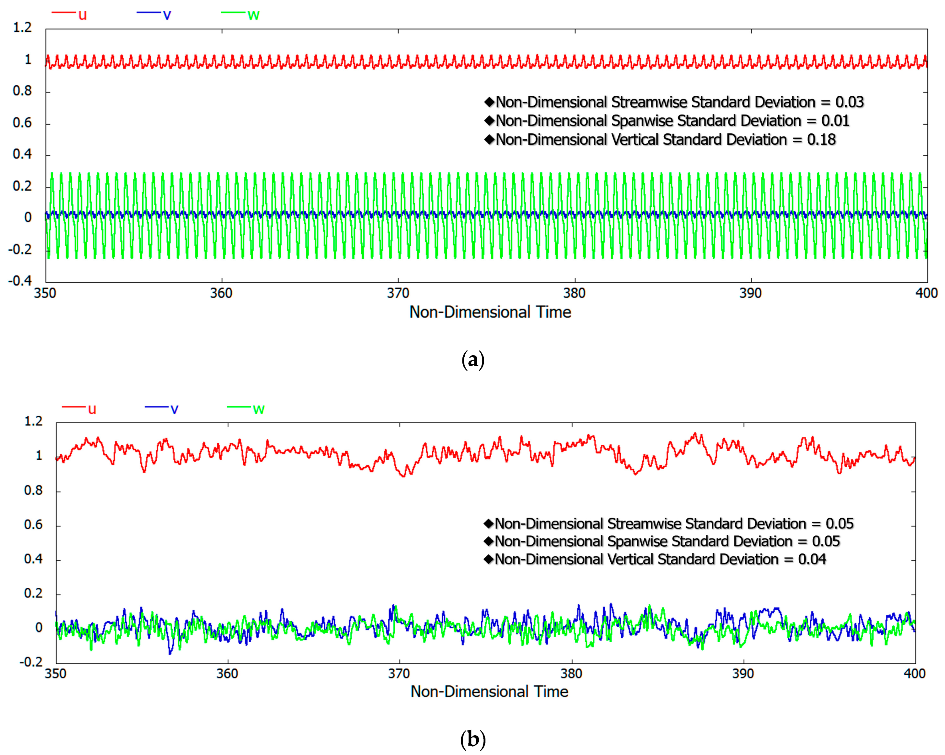
Figure 15 shows the time variation of the three velocity components at the N = 4 measurement points (x = 0.5 D and z = 0.5 D, x = 30.0 D and z = 0.5 D) shown in
Figure 14a (the mid-span plane and at the top-tip height). The current paper imposes inflow condition with no turbulent fluctuations. Therefore, at x = 0.5 D in the near-wake region shown in
Figure 15a, a waveform that reflected the behavior of the tip vortex that was periodically formed and shed was clearly observed, as described above. On the other hand, at x = 30.0 D in the far-wake region shown in
Figure 15b, it could be seen that the three velocity components greatly fluctuated, reflecting the vertical meandering motion. We considered that the mechanism by which the periodic shedding of the tip vortex formed from the tip of the wind-turbine blade collapsed, due to the instability of the strong velocity shear in the distance of the wind turbine, and the vertical meandering motion in the far-wake region subsequently formed. Due to the inflow condition with no turbulent fluctuations, the periodic generation and shedding of tip vortex and the subsequent collapse of tip vortex caused by shear instability directly affect the meandering motion in the far-wake region [
12,
13].
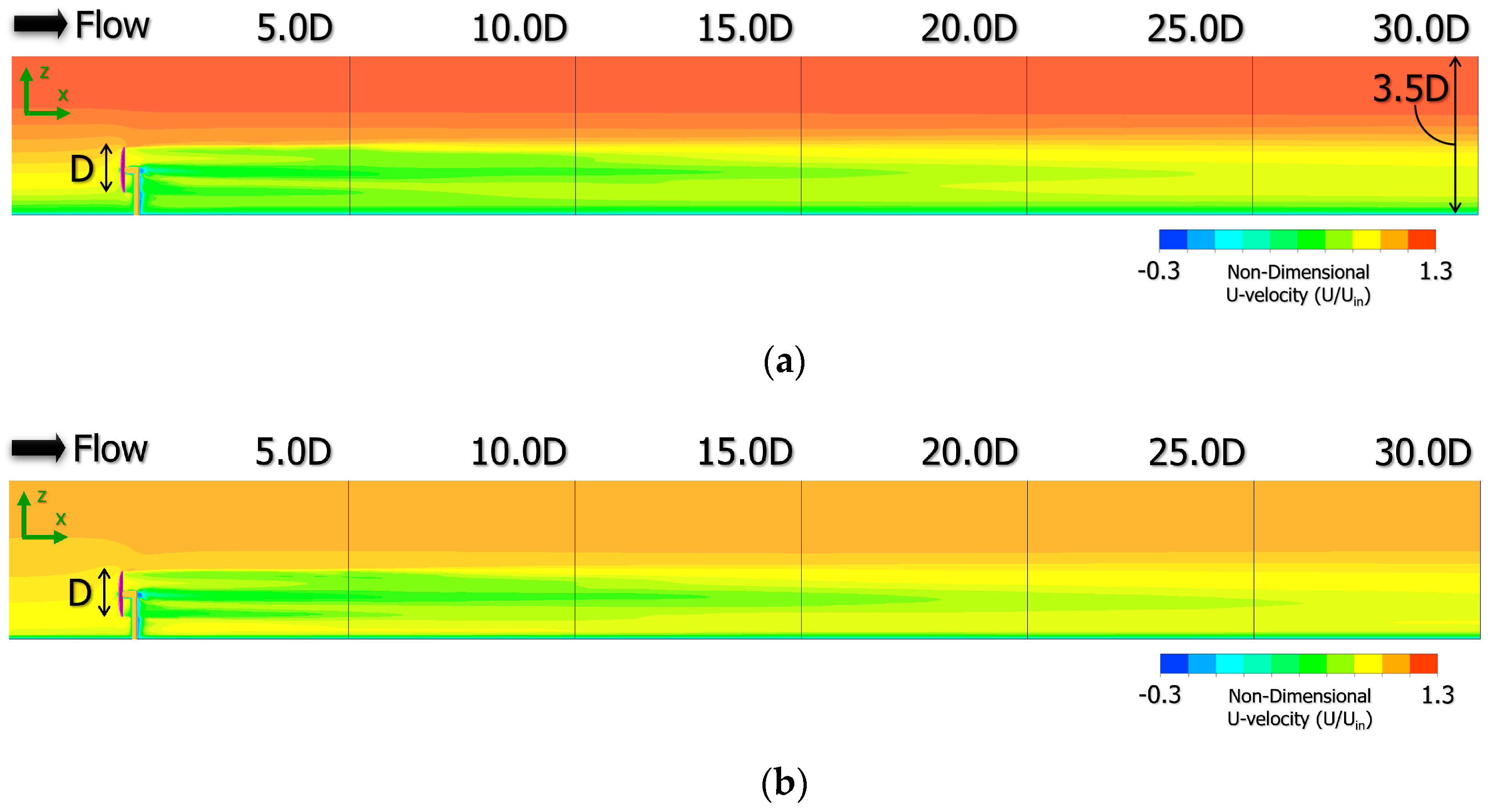
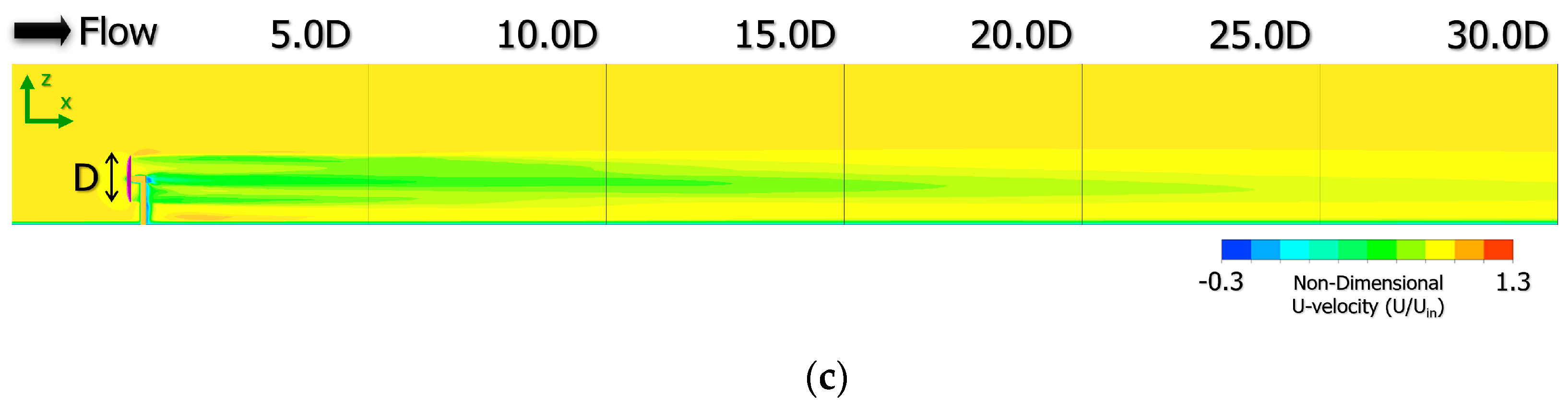
Figure 16 shows the spatial distribution of U-velocity in the mid-span plane (side view) for the time-averaged field calculated at t = 200–400 R/U
in. First, as expected, the periodic shedding of the tip vortex observed in
Figure 14 disappeared with temporal averaging. On the other hand, it was clear that the decay of the wake velocity deficit in the far-wake region behind a wind-turbine clearly existed, even 30 times downstream of the diameter of the wind-turbine. The wind velocity deficit near the hub center was almost the same in all cases regardless of difference in inflow shear.
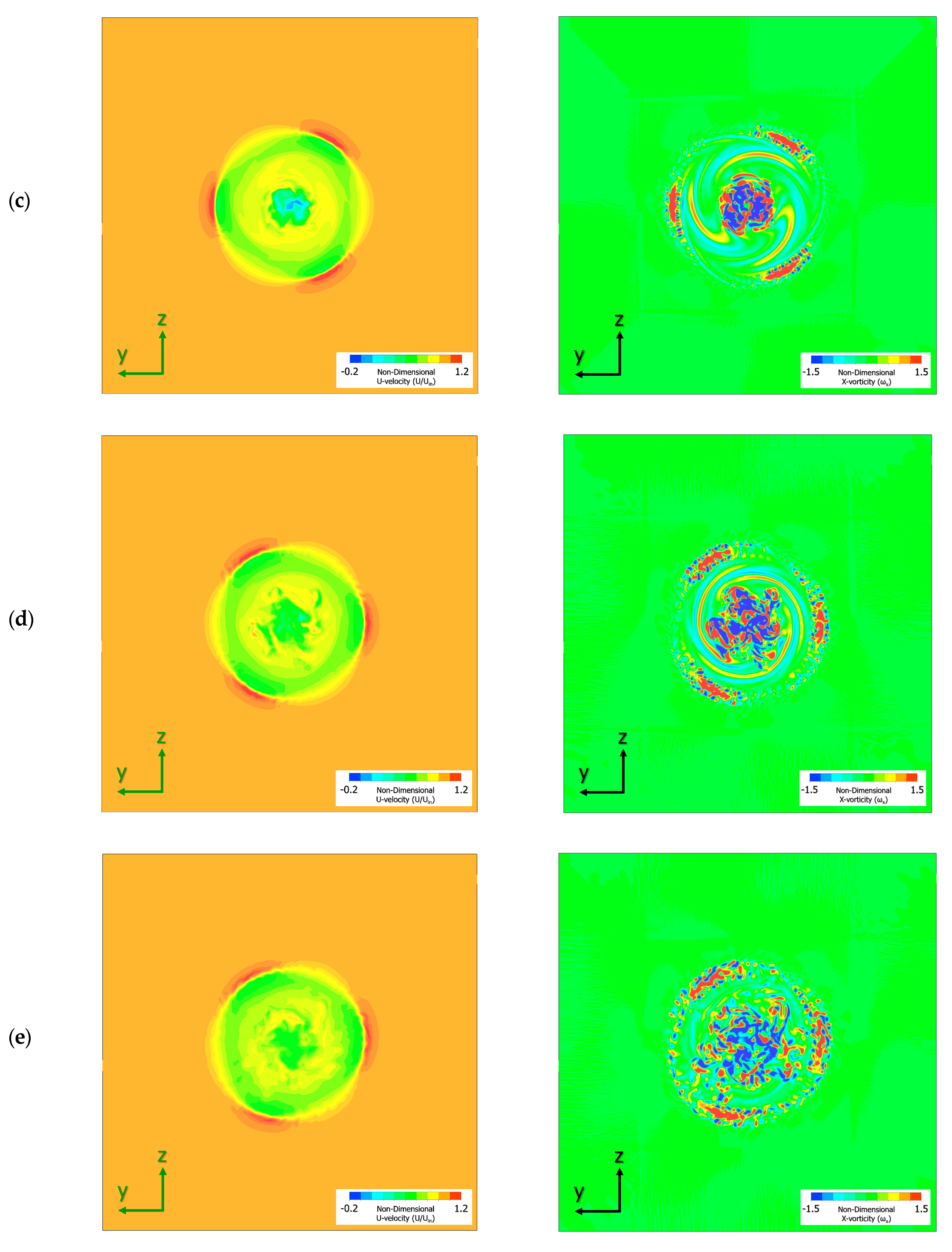
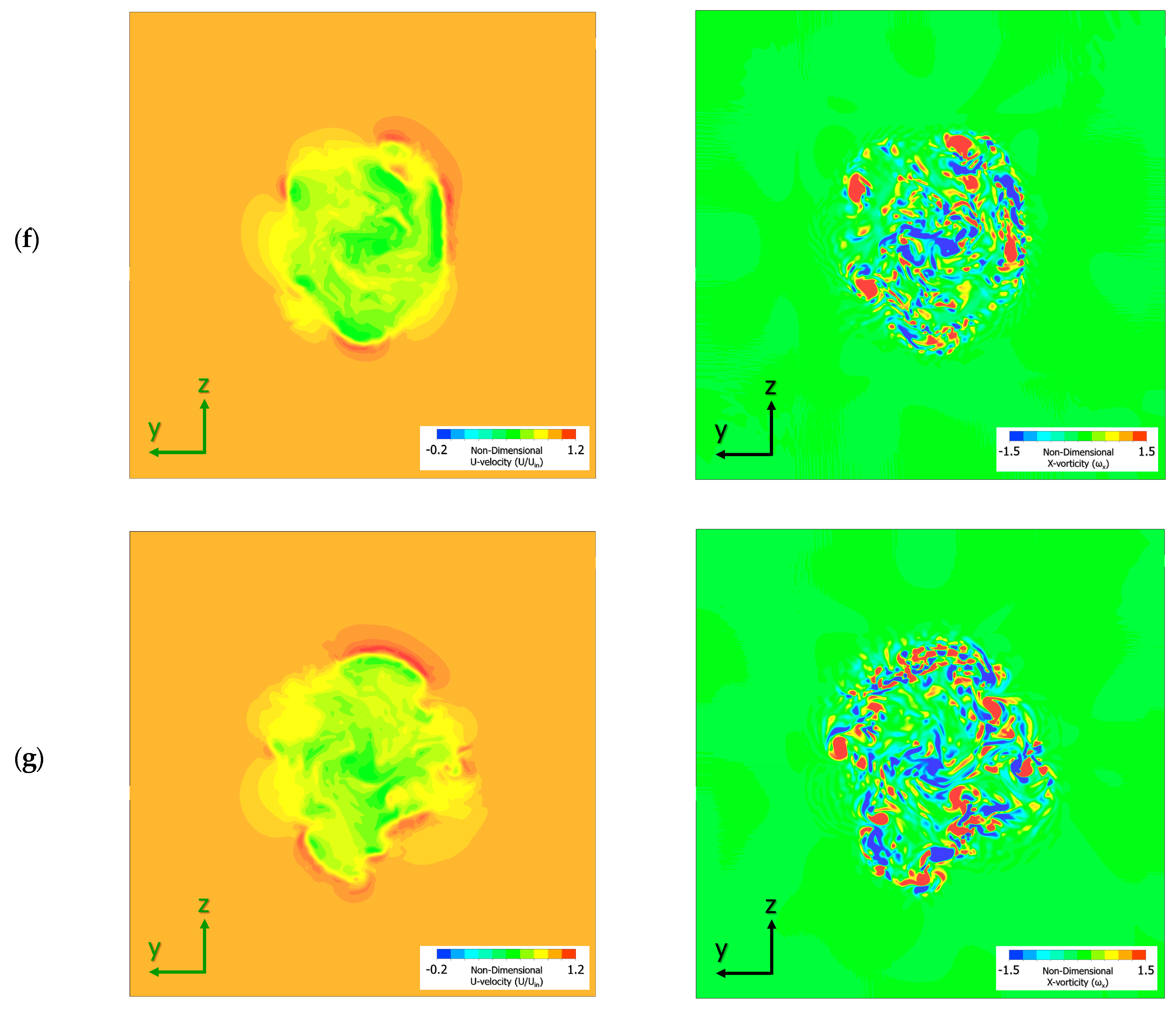
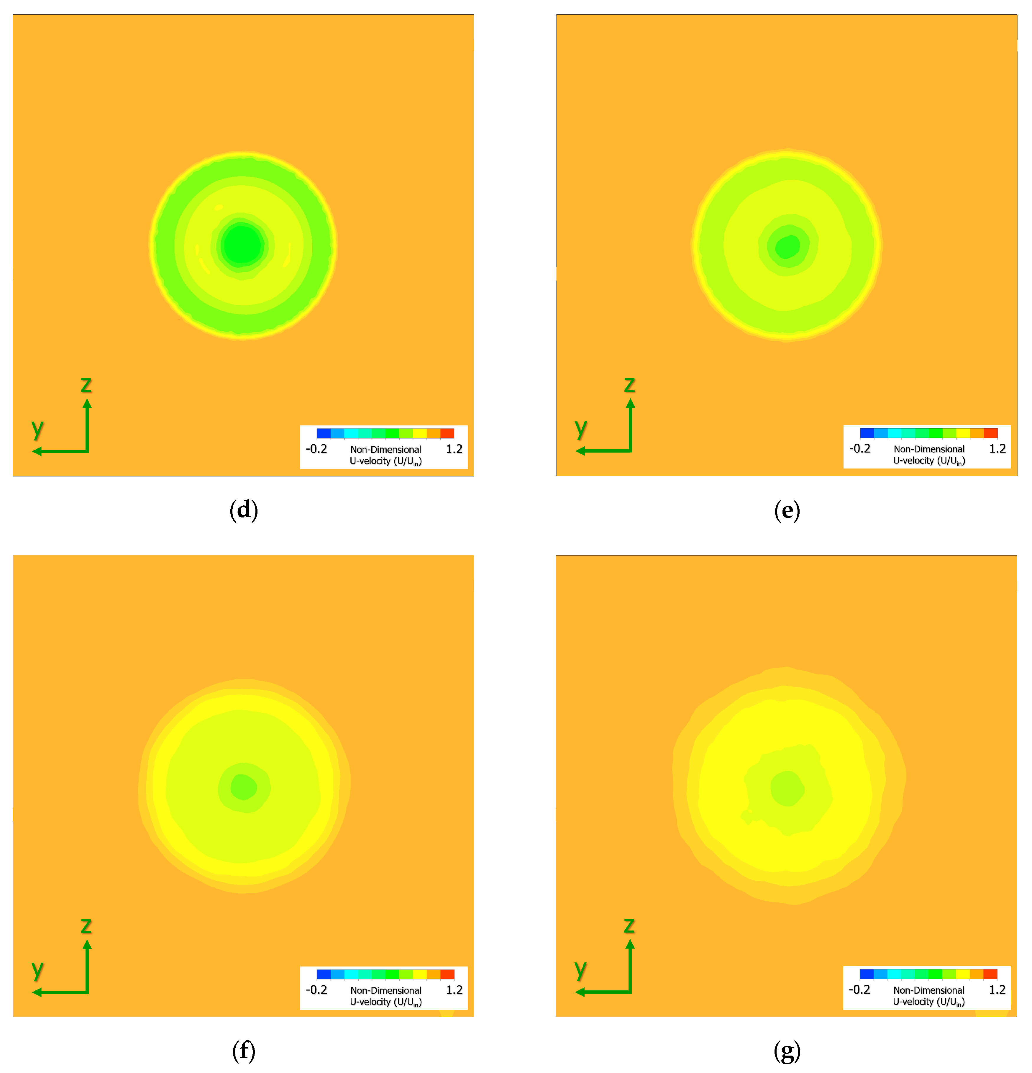
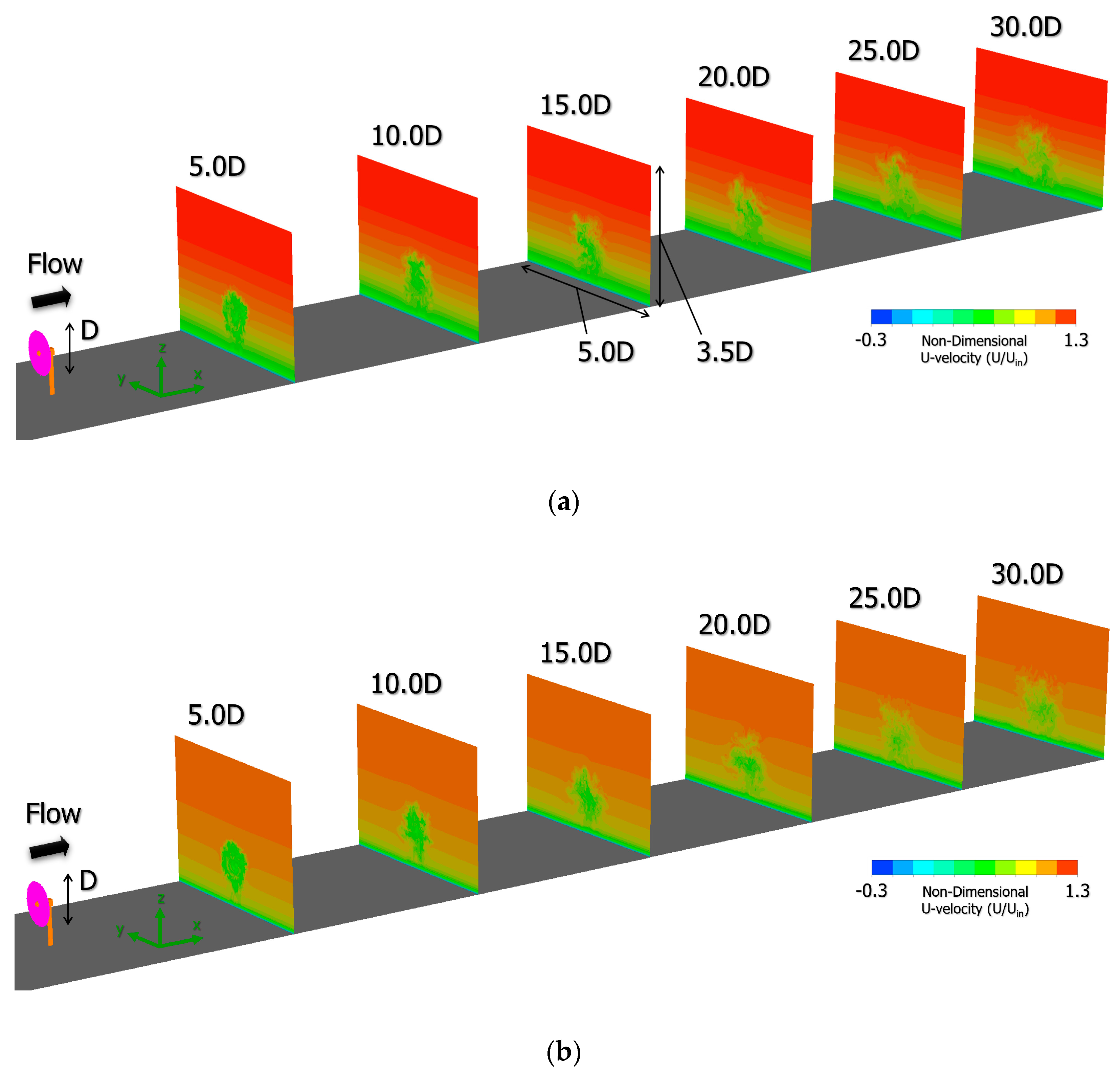
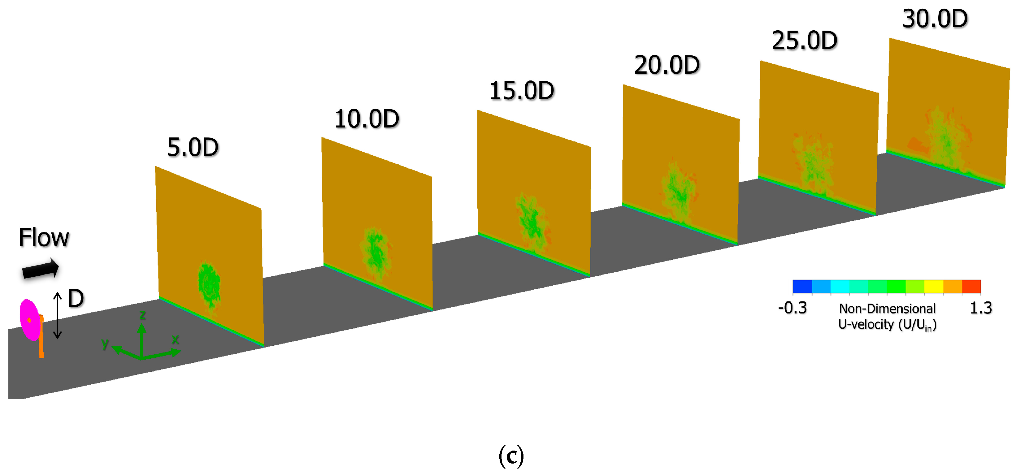
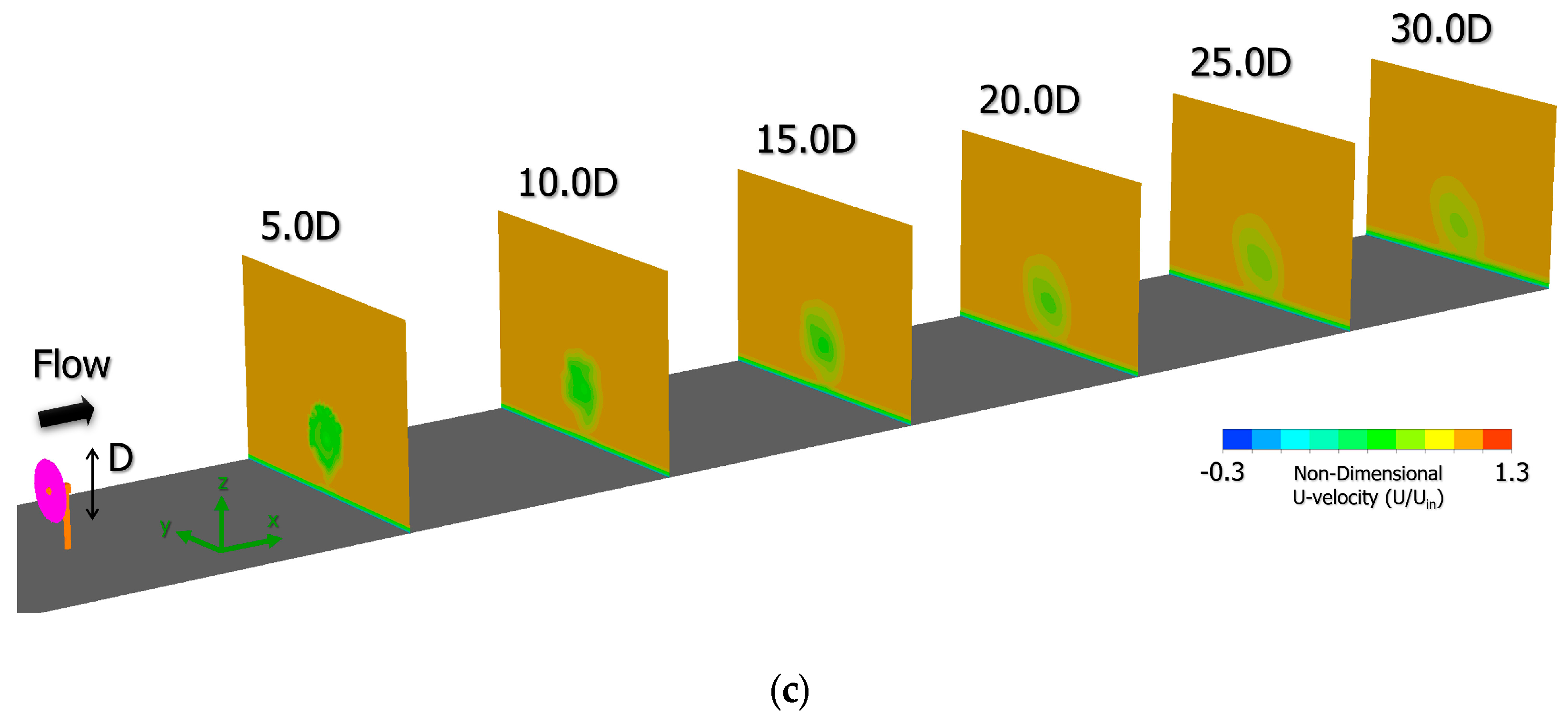
Figure 17 shows the spatial distribution of U-velocity in the y–z plane (front view) at x = 5.0 D to 30.0 D for the instantaneous flow field of t = 400 R/U
in. In all cases of N = 4 shown in
Figure 17a, N = 10 shown in
Figure 17b, and uniform flow shown in
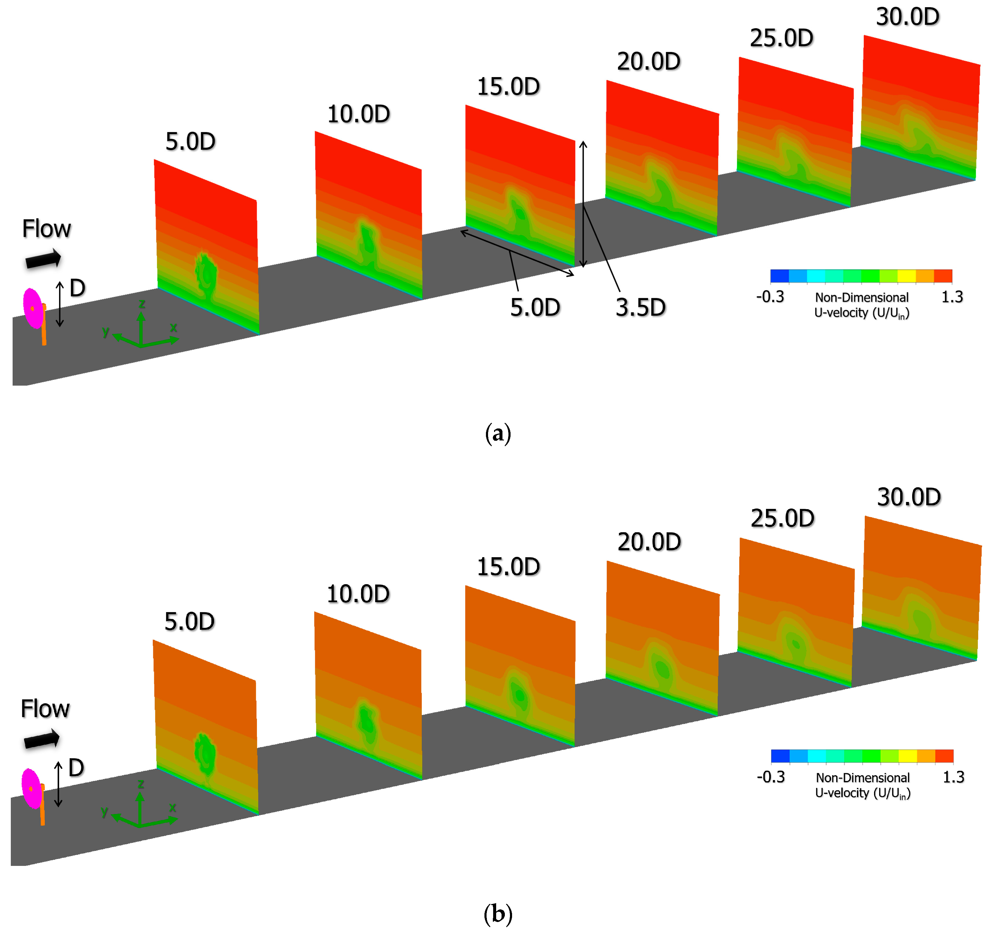
Figure 17c, an almost concentric wake region was formed behind the wind-turbine in the near-wake region with x = 5.0 D. In the far-wake region of x ≥ 10.0 D, the concentric wake region was greatly deformed with the occurrence of the vertical meandering motion. In the visualization result (
Figure 18) for the time-averaged flow field corresponding to
Figure 17, the distortion of wake flows in the far-wake region with x ≥ 10.0 D also clearly existed. As described above,
Figure 18 also shows that the wind velocity deficit near the hub center of the wind-turbine was almost the same in all cases, regardless of the difference in inflow shear.
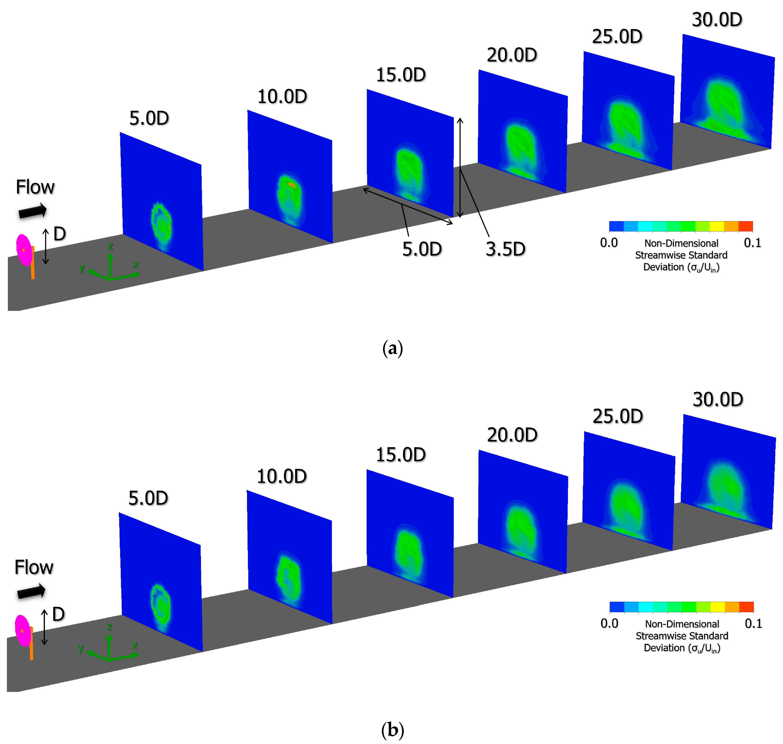
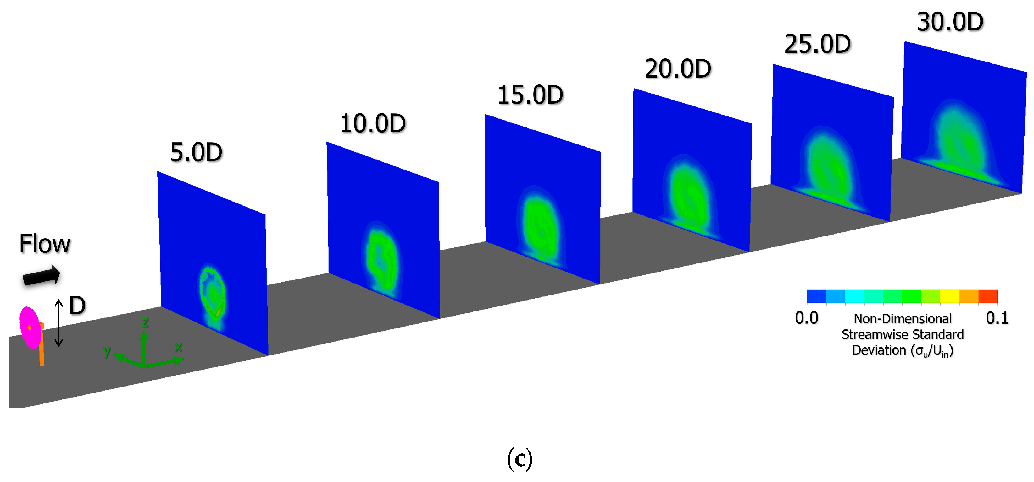
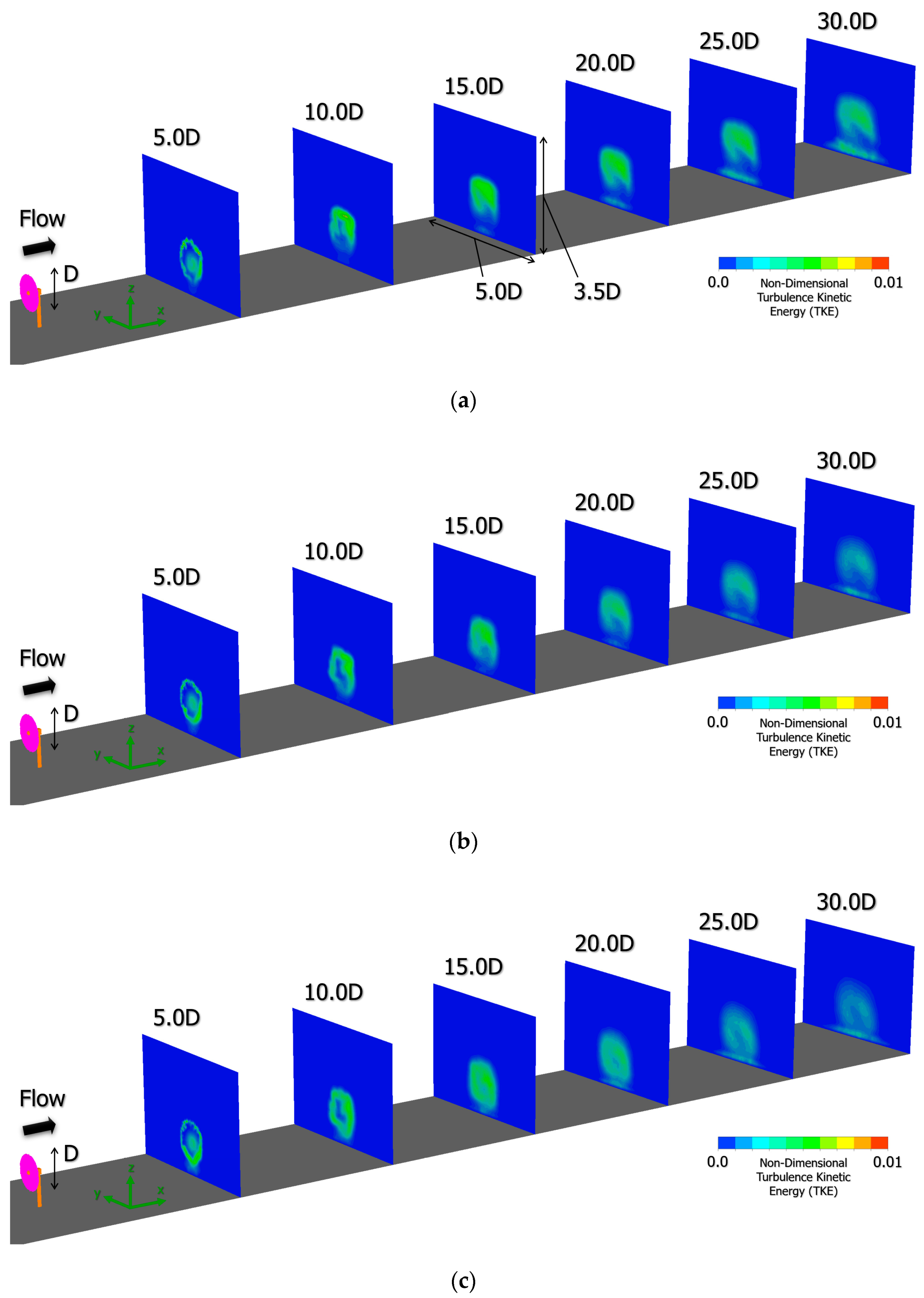
Figure 19 shows the spatial distribution of nondimensional streamwise standard deviation in the y–z plane (front view) at x = 5.0 D to 30.0 D. Regardless of the difference in velocity shear, spatial distribution was almost the same at each x coordinate position. We also examined the spatial distribution of turbulence kinetic energy (TKE) corresponding to
Figure 19. The results are shown in
Appendix E. In
Figure 19 and
Figure 20, the discernible difference in the flow fields depending on the sheared and uniform inflow conditions could not be observed clearly.
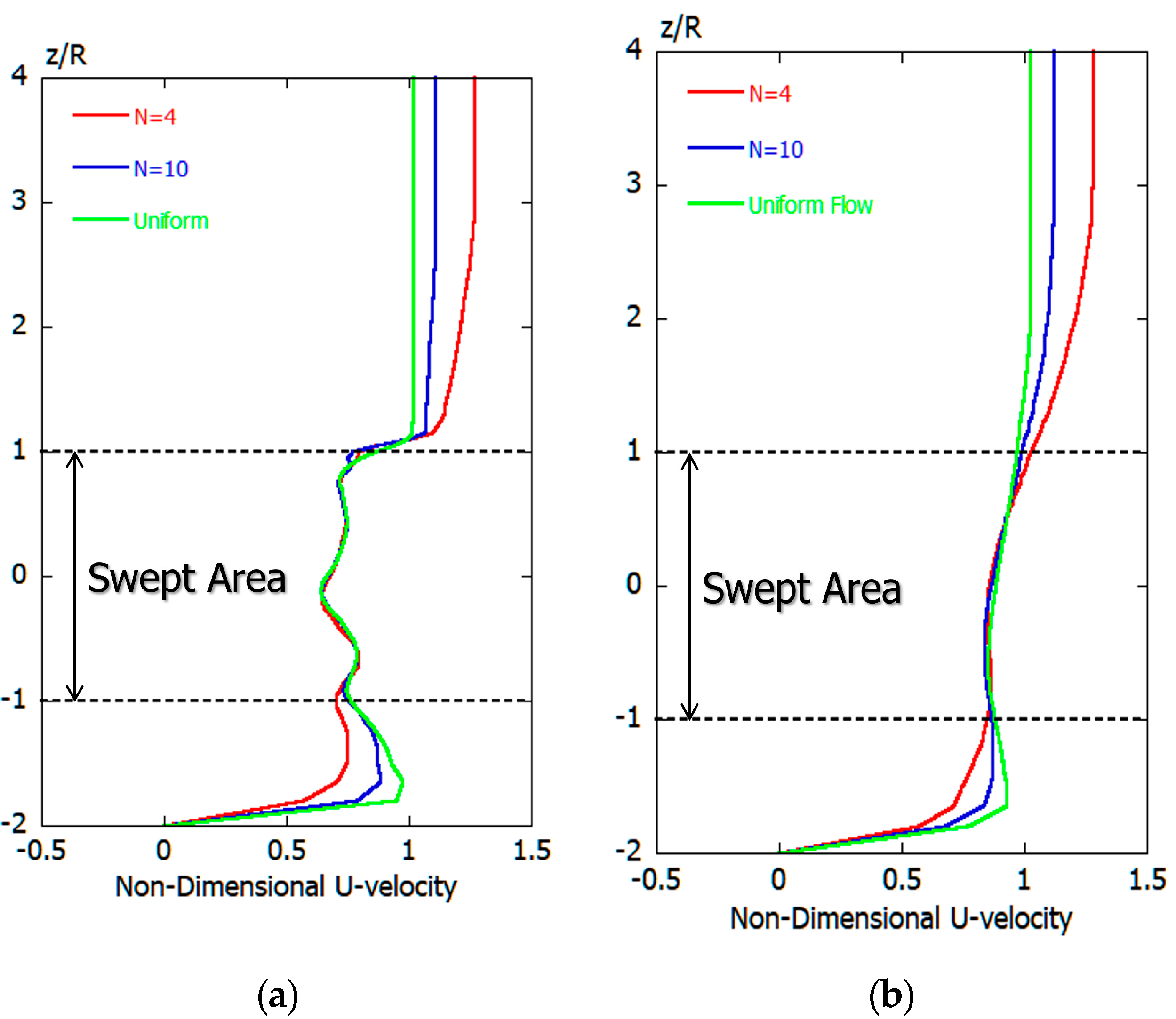
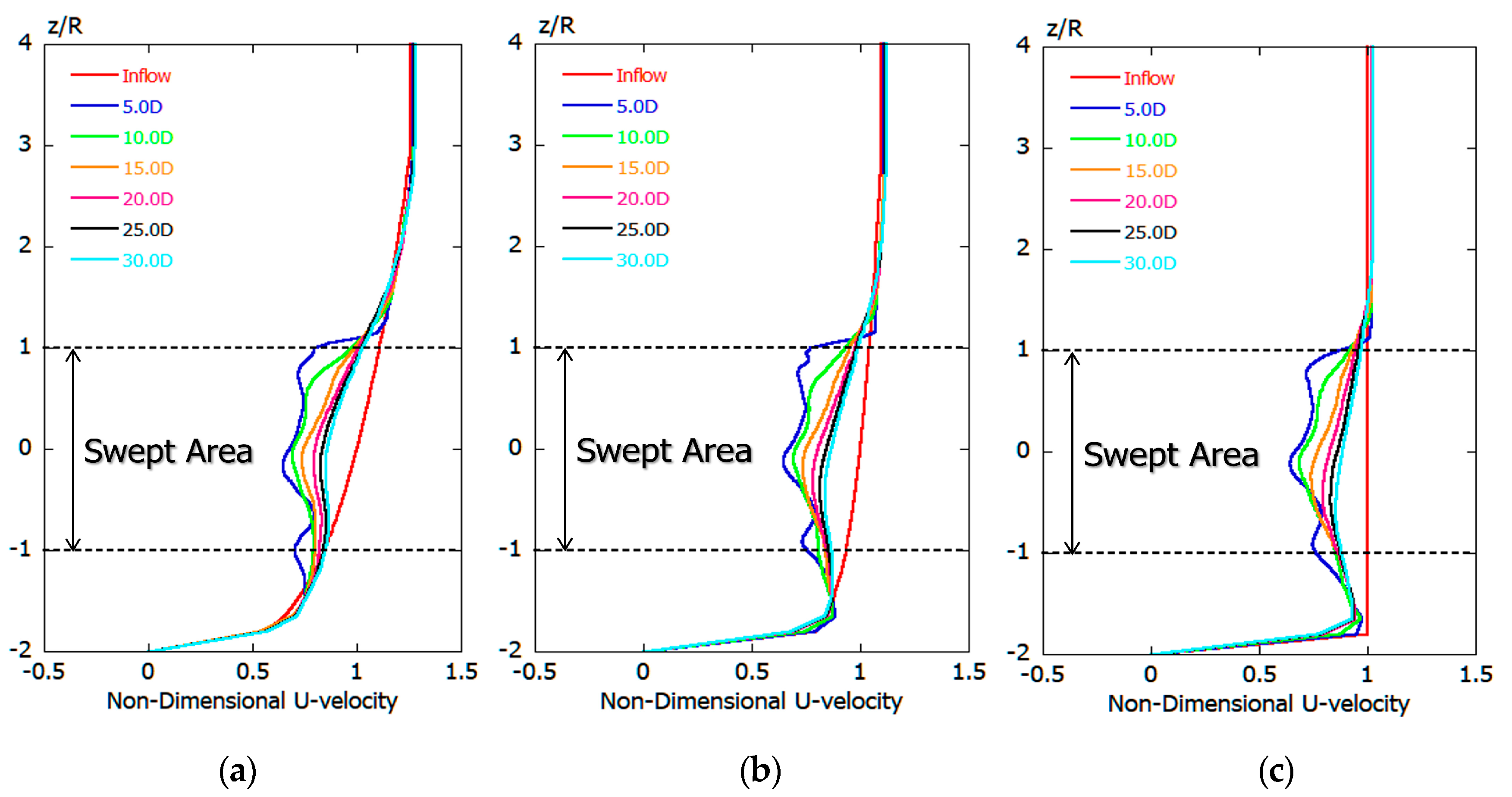
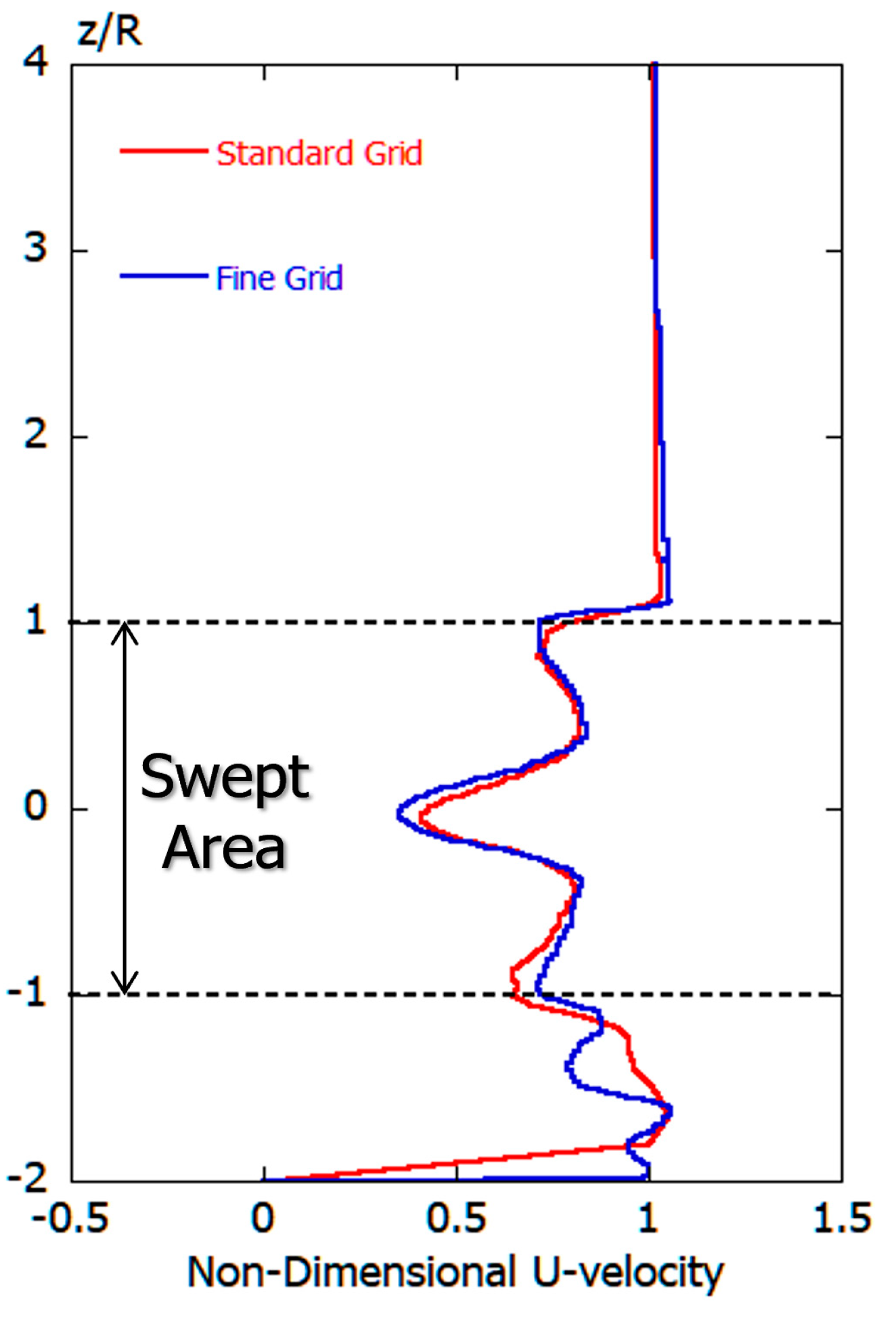
Figure 20 shows a comparison of vertical distribution of time-averaged U-velocity at x = 5.0 D and 30.0 D. It is very interesting that, regardless of difference in inflow shear, the vertical distribution of time-averaged U-velocity showed almost the same tendency in the entire swept area of the wind-turbine at both x = 5.0 D and 30.0 D. At x = 5.0 D in the near-wake region shown in
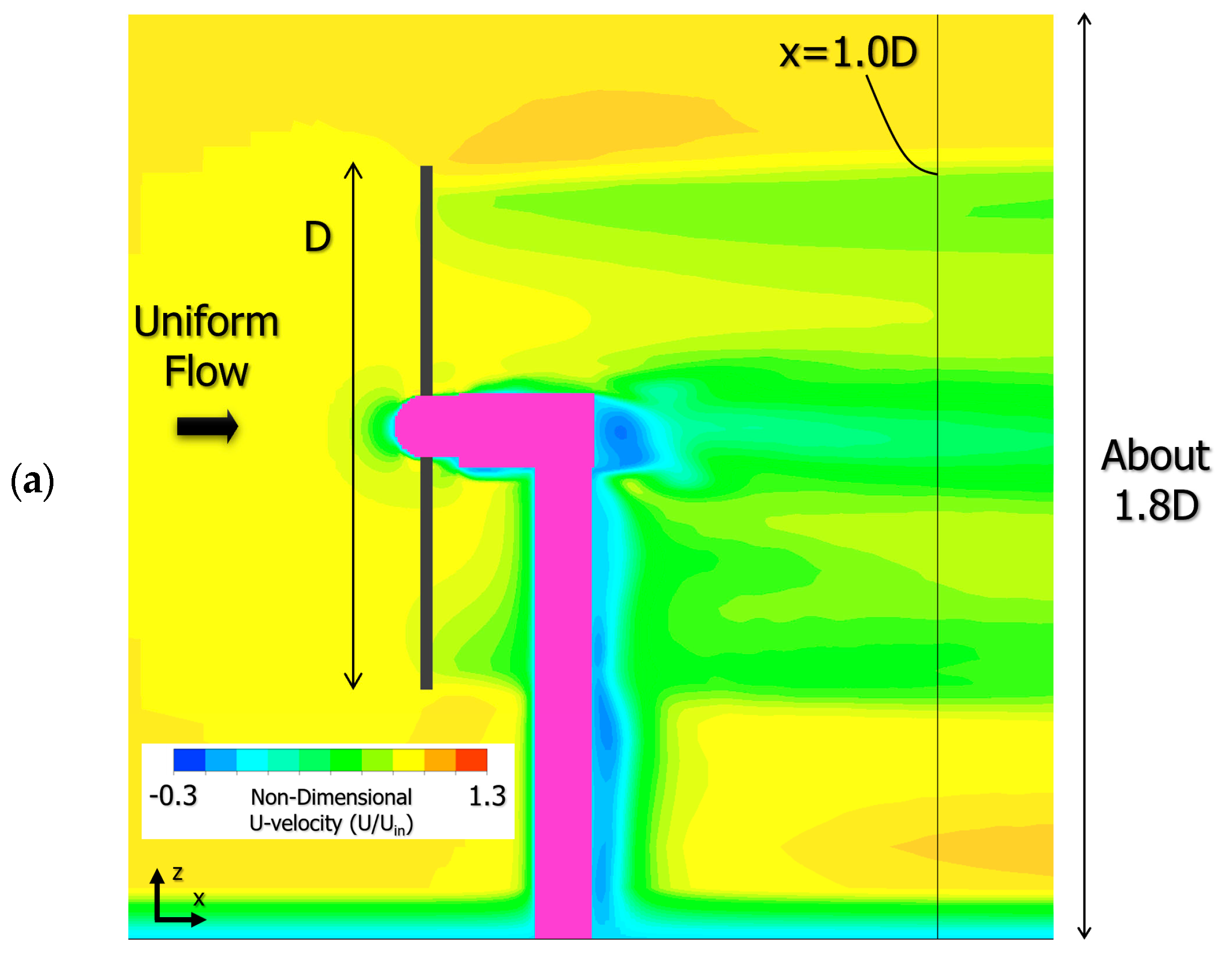
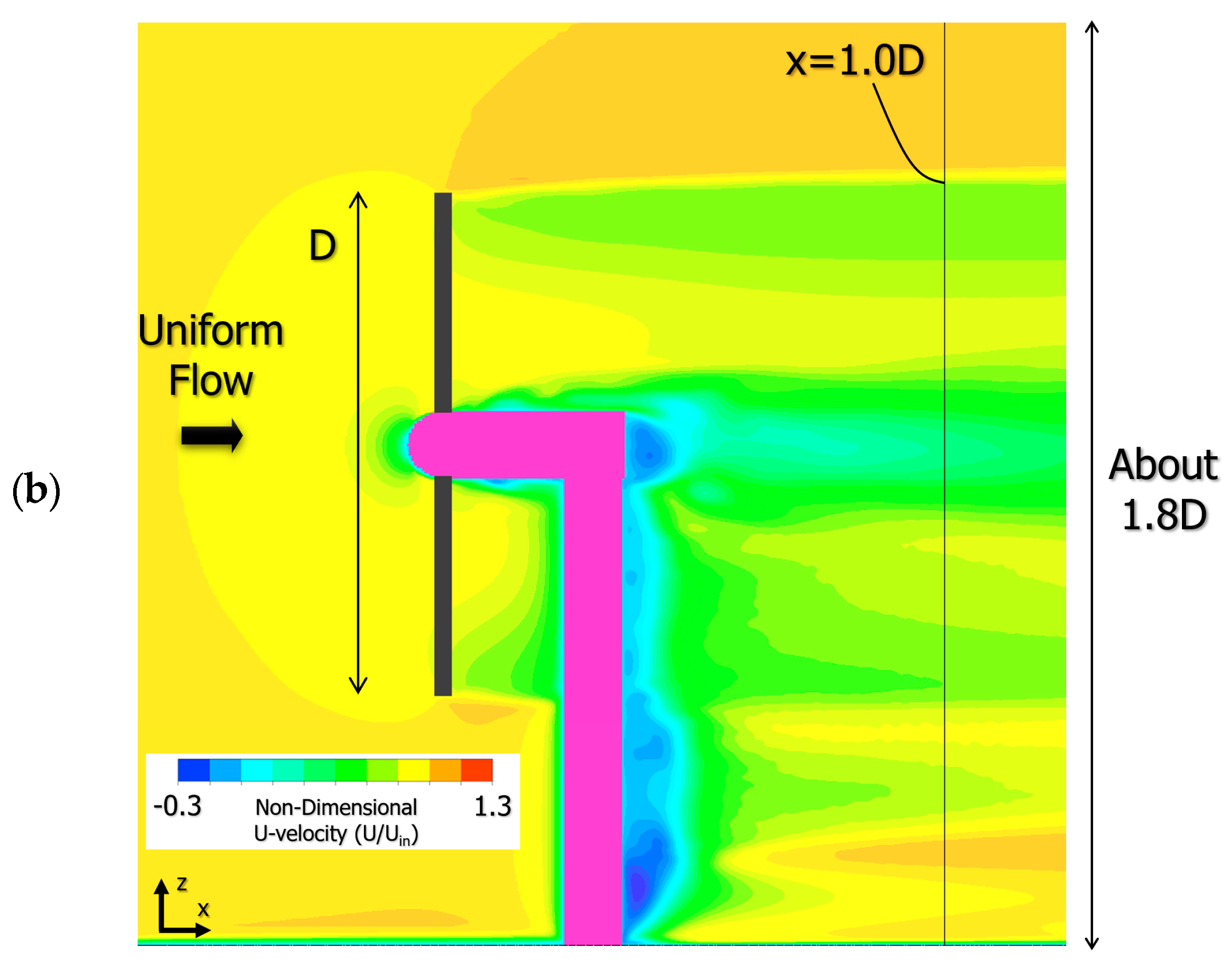
Figure 20a, a large velocity shear occurred at z/R = 1 in all cases, as described above. The time-averaged U-velocity exhibited sharp corners below the swept area (especially in the case of the uniform flow). This means that the flow here is locally accelerated. We performed additional calculations using very fine grid, and investigated the reason for this flow phenomenon. The results are shown in
Appendix D. On the other hand, at x = 30.0 D in the far-wake region shown in
Figure 20b, an approximately conical wake profile was formed in all cases of N = 4, N = 10, and uniform flow. We arranged the vertical distribution of time-averaged U-velocity for every three cases of N = 4, N = 10, and uniform flow. The results are shown in
Appendix A.
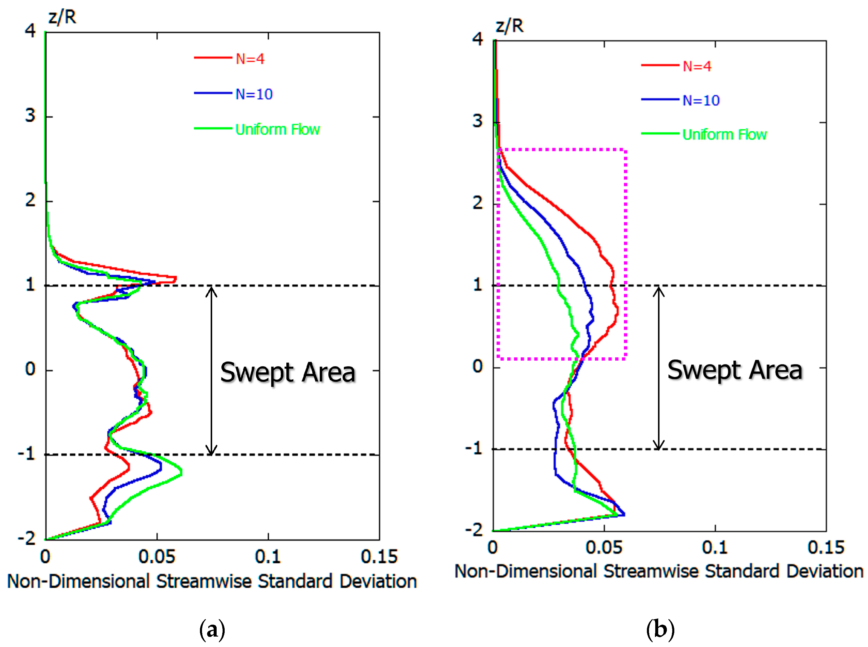
Figure 21 shows the comparison of vertical distribution of nondimensional streamwise standard deviation at x = 5.0 and 30.0 D, corresponding to
Figure 20. At x = 5.0 D in the near-wake region shown in
Figure 21a, almost the same numerical values were shown in the entire swept area of the wind-turbine, regardless of the difference in speed shear. At the top position of the wind-turbine blade, z/R = 1, and at the bottom position of the wind-turbine blade, z/R = −1, maximal values are clearly shown. The maxima at these two locations are due to the passage of the periodically formed tip vortex. On the other hand, the differences within the swept area for different values of shear are significant at x = 30.0 D (see dotted line in
Figure 21b).
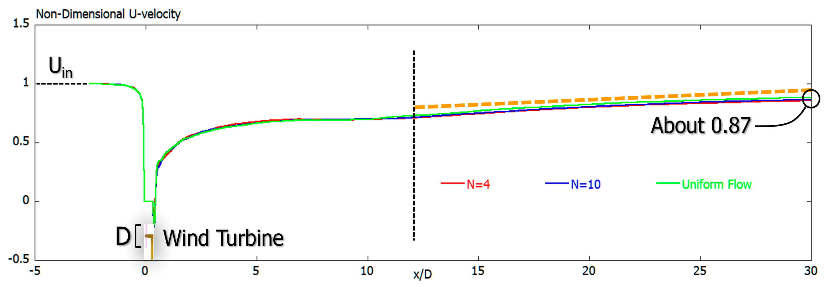
Figure 22 shows a comparison of time-averaged U-velocity distribution at the hub center of the wind-turbine. As described above, time-averaged U-velocity distribution at the hub center of the wind-turbine behaved in almost the same way in all three cases, regardless of differences in inflow shear. In all three cases, the wake velocity deficit in the far-wake region behind a wind-turbine gradually and linearly recovered with x, and its recovery rate was very small. As shown by the orange dotted line in the figure, the recovery rate changed in the far-wake region of x ≥ 12.0 D. This was thought to be due to the occurrence of vertical meandering motion in the far-wake region and the increase in vertical fluctuation. In all cases, 10% velocity deficit was clearly present even in the far-wake region of x = 30.0 D, as shown in the figure.
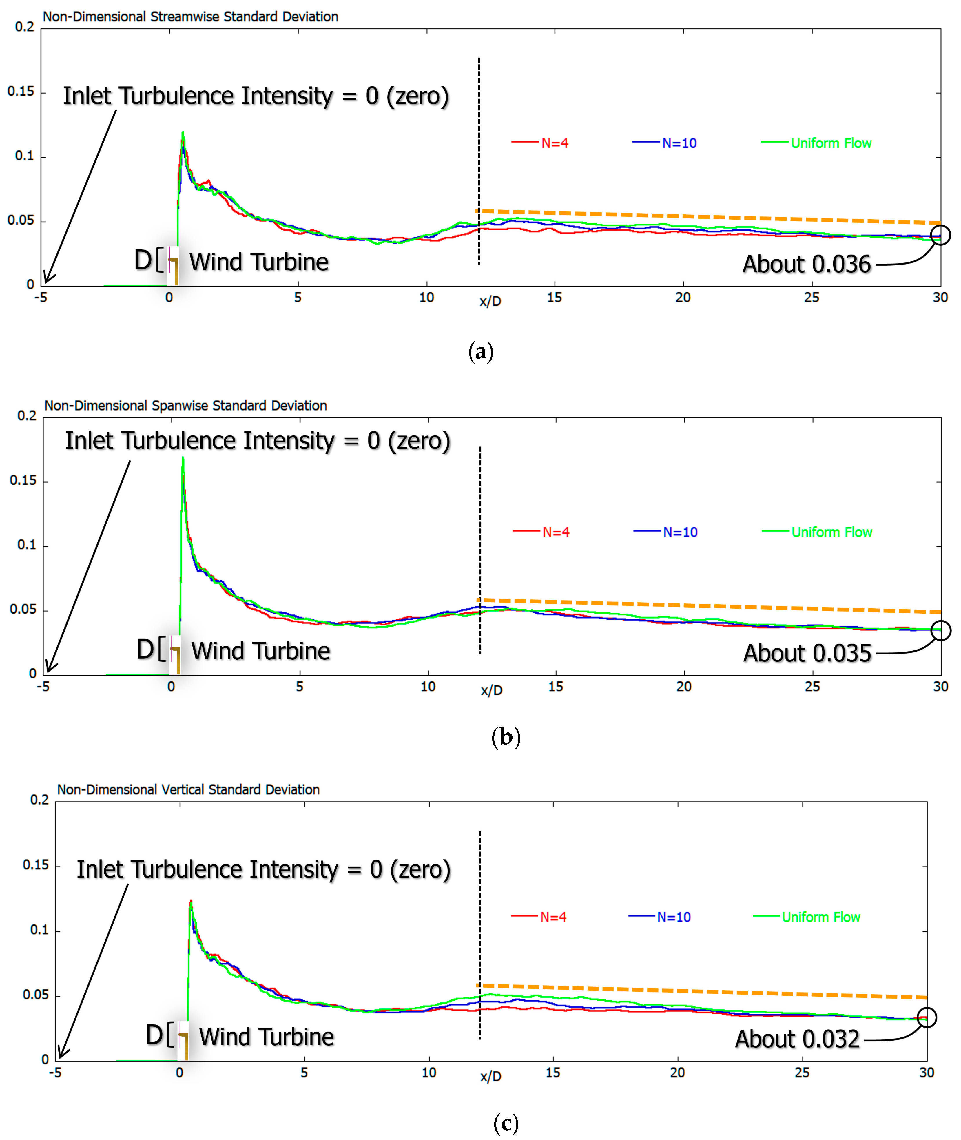
Figure 23 shows a comparison of nondimensional standard deviation distribution at the hub center of the wind-turbine, corresponding to
Figure 22. Similar to
Figure 22, the nondimensional standard deviation distribution at the hub center of the wind-turbine showed almost the same values in all cases of
Figure 23a–c, regardless of difference in inflow shear. Furthermore, as in
Figure 23, the slope at which the nondimensional standard deviation decayed changed in the far-wake region of x ≥ 12.0 D. As shown in the figure, the numerical value at x = 30.0 D in the far-wake region gradually decreased in the order of the (a) streamwise, (b) spanwise, and (c) vertical directions. There are some points to note here. As shown in
Figure 21b, in the far-wake region, there is a significant difference in standard deviation, especially in the upper part of the swept area, due to the influence of inflow shear.
4. Conclusions
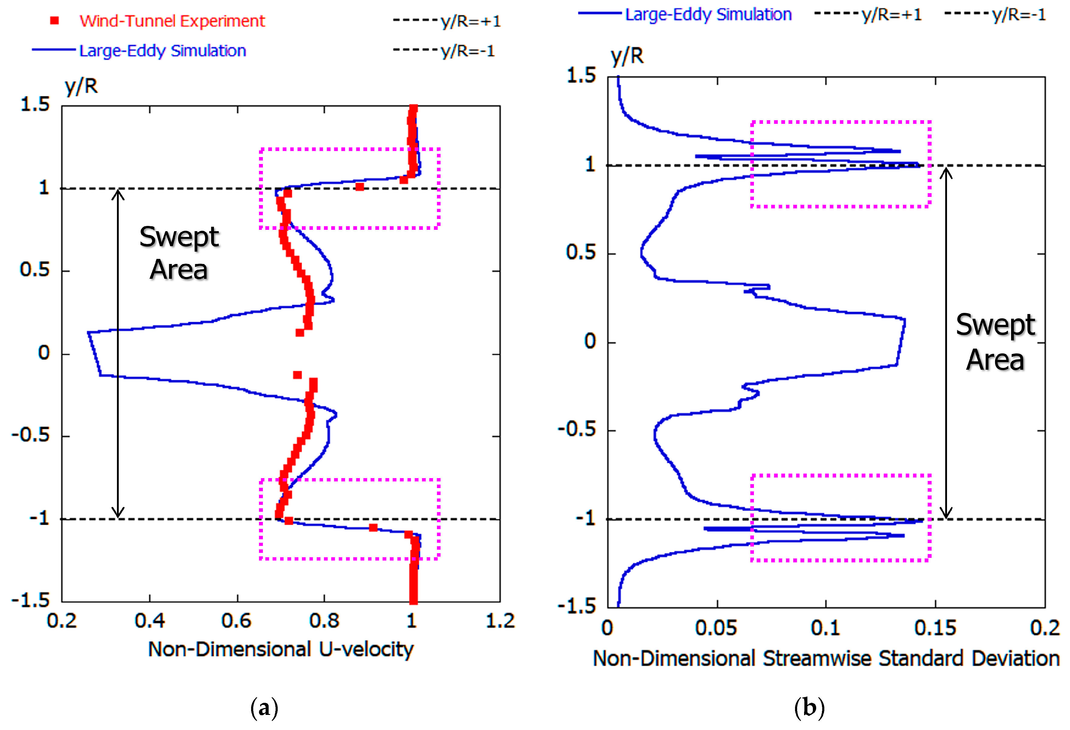
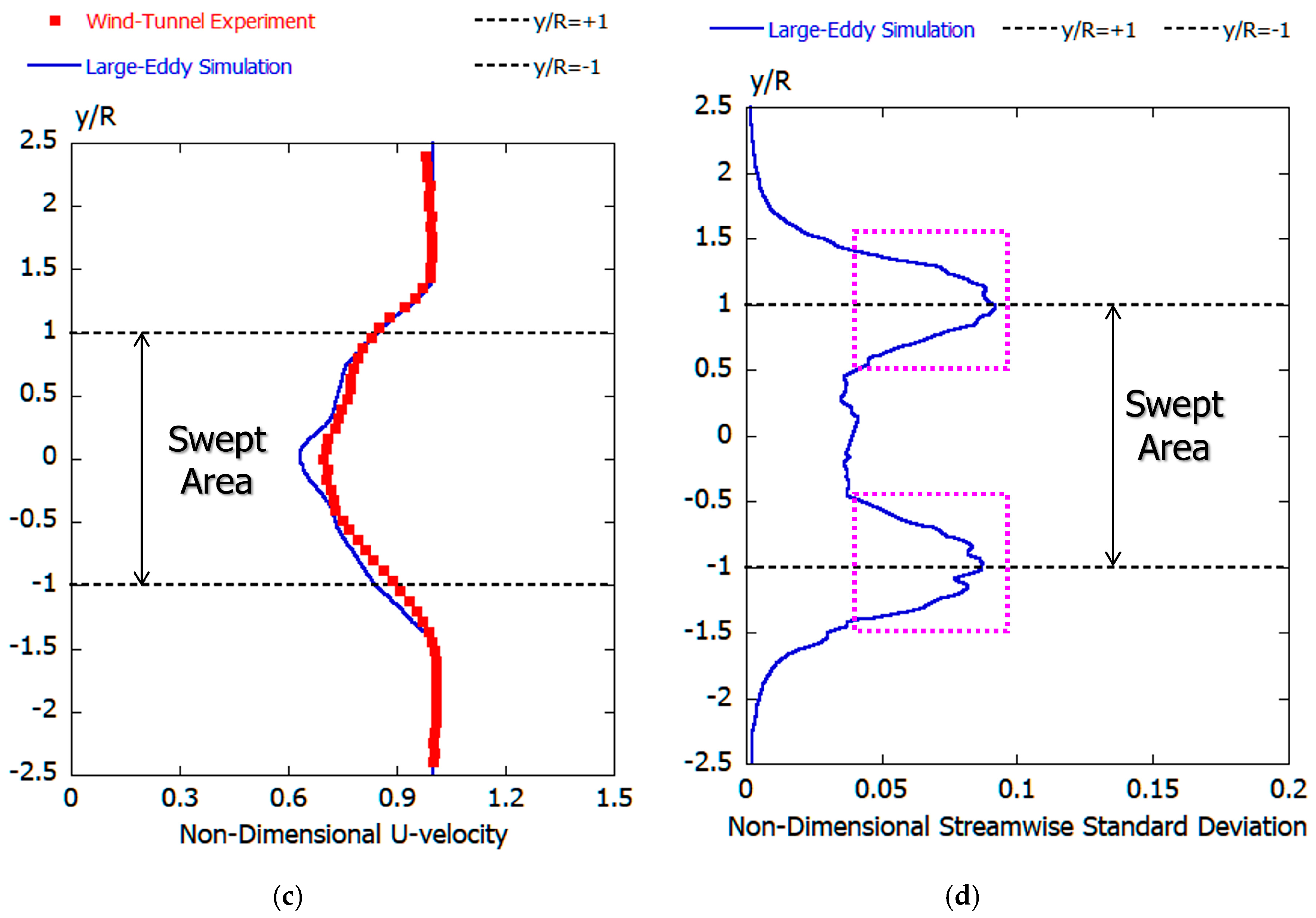
The scope of the present study was to understand the wake characteristics of wind-turbines under various inflow shears. First, in order to verify the prediction accuracy of RIAM-COMPACT, the in-house LES solver based on a Cartesian staggered grid, we conducted a wind-tunnel experiment using a wind-turbine scale model and compared the numerical and experimental results. The total number of grid points in the computational domain was about 235 million. Parallel computation based on a hybrid LES/AL model approach was performed with a new SX-Aurora TSUBASA vector supercomputer. From the comparison between the wind-tunnel experiment and the high-resolution LES results, the AL model that was implemented in the in-house LES solver in this study could accurately reproduce both the performance of the wind-turbine scale model and the flow characteristics in the wake region.
Next, using the LES solver developed in-house, the flow past the entire wind-turbine, including the nacelle and the tower, was simulated for a tip speed ratio of 4, the optimal TSR with a new SX-Aurora TSUBASA vector supercomputer. Three types of inflow shear, namely, N = 4, N = 10, and uniform flow, were set at the inflow boundary. In these calculations, the calculation domain in the streamwise direction was very long, 30.0 D (D being the wind-turbine rotor diameter) from the center of the wind-turbine hub. Therefore, long-term integration of t = 0 to 400 R/Uin was performed. Various turbulence statistics were calculated at t = 200 to 400 R/Uin. Here, R is the wind-turbine rotor radius, and Uin is the wind speed at the hub center height. On the basis of the obtained results, we numerically investigated the effects of inflow shear on the wake characteristics of wind-turbines over a flat terrain.
Focusing on the center of the wind-turbine hub, all results showed almost the same behavior regardless of difference in the three types of inflow shear. In all cases, 10% velocity deficit was clearly present even in the far-wake region of x = 30.0 D. The nondimensional standard deviation distribution at the hub center of the wind-turbine showed almost the same values in all cases, regardless of difference in inflow shear. Furthermore, the slope at which the nondimensional standard deviation decayed changed in the far-wake region of x ≥ 12.0 D. The numerical value at x = 30.0 D in the far-wake region gradually decreased in the order of the (a) streamwise, (b) spanwise, and (c) vertical directions.
Through the comparison of vertical distribution of time-averaged U-velocity at x = 5.0 D and 30.0 D, we obtained the following findings. It is very interesting that, regardless of difference in inflow shear, the vertical distribution of time-averaged U-velocity showed almost the same tendency in the entire swept area of the wind-turbine at both x = 5.0 D and 30.0 D. At x = 5.0 D in the near-wake region, a large velocity shear occurred at z/R = 1 in all cases. On the other hand, at x = 30.0 D in the far-wake region, an approximately conical wake profile was formed in all cases of N = 4, N = 10, and uniform flow.
Regarding the comparison of vertical distribution of nondimensional streamwise standard deviation at x = 5.0 and 30.0 D, the following findings were obtained. At x = 5.0 D in the near-wake region, almost the same numerical values were shown in the entire swept area of the wind-turbine, regardless of the difference in speed shear. At the top position of the wind-turbine blade and at the bottom position of the wind-turbine blade, maximal values are clearly shown. The maxima at these two locations are due to the passage of the periodically formed tip vortex. On the other hand, the differences within the swept area for different values of shear are significant at x = 30.0 D.


