Article

Development and Calibration of a Semianalytic Model for Shale Wells with Nonuniform Distribution of Induced Fractures Based on ES-MDA Method

1
Key Laboratory of Tectonics and Petroleum Resources, Ministry of Education, China University of Geosciences, Wuhan 430074, China
2
School of Earth Resources, China University of Geosciences, Wuhan 430074, China
3
State Key Laboratory of Geomechanics and Geotechnical Engineering, Institute of Rock and Soil Mechanics, Chinese Academy of Sciences, Wuhan 430071, China
4
Institute of Geophysics and Geomatics, China University of Geosciences, Wuhan 430074, China
*
Author to whom correspondence should be addressed.
Energies 2020, 13(14), 3718; https://doi.org/10.3390/en13143718
Submission received: 22 June 2020 / Revised: 16 July 2020 / Accepted: 16 July 2020 / Published: 20 July 2020
(This article belongs to the Special Issue Development of Unconventional Reservoirs 2020)

Abstract

:
Given reliable parameters, a newly developed semianalytic model could offer an efficient option to predict the performance of the multi-fractured horizontal wells (MFHWs) in unconventional gas reservoirs. However, two major challenges come from the accurate description and significant parameters uncertainty of stimulated reservoir volume (SRV). The objective of this work is to develop and calibrate a semianalytic model using the ensemble smoother with multiple data assimilation (ES-MDA) method for the uncertainty reduction in the description and forecasting of MFHWs with nonuniform distribution of induced fractures. The fractal dimensions of induced-fracture spacing (dfs) and aperture (dfa) and tortuosity index of induced-fracture system (θ) are included based on fractal theory to describe the properties of SRV region. Additionally, for shale gas reservoirs, gas transport mechanisms, e.g., viscous flow with slippage, Knudsen diffusion, and surface diffusion, among multi-media including porous kerogen, inorganic matter, and fracture system are taken into account and the model is verified. Then, the effects of the fractal dimensions and tortuosity index of induced fractures on MFHWs performances are analyzed. What follows is employing the ES-MDA method with the presented model to reduce uncertainty in the forecasting of gas production rate for MFHWs in unconventional gas reservoirs using a synthetic case for the tight gas reservoir and a real field case for the shale gas reservoir. The results show that when the fractal dimensions of induced-fracture spacing and aperture is smaller than 2.0 or the tortuosity index of induced-fracture system is larger than 0, the permeability of induced-fracture system decreases with the increase of the distance from hydraulic fractures (HFs) in SRV region. The large dfs or small θ causes the small average permeability of the induced-fracture system, which results in large dimensionless pseudo-pressure and small dimensionless production rate. The matching results indicate that the proposed method could enrich the application of the semianalytic model in the practical field.

1. Introduction

Unconventional reservoirs, especially the tight sand and shale reservoirs, have become more and more significant with the development of the horizontal wells and hydraulic fracturing technologies. The complex fracture network surrounding the multistage fractured horizontal wells (MFHWs) called stimulated reservoir volume (SRV), has obvious influences on the production performance [1,2,3]. Currently, a lot of effort has been done to model the pressure transient and rate transient of MFHWs aiming to forecast the production accurately. Through numerical methods, analytical methods, and empirical methods [4,5,6,7], production data analysis in unconventional reservoirs, such as Barnett, Bakken, and Eagle, shows that the linear flow in formation, especially in hydraulic fractures (HFs) and SRV, dominates the production of MFHWs. Meanwhile, the advantage of analytic models is their simplicity and less parameters compared with numerical and empirical models, although they cannot characterize the over-complex heterogeneity properties and fracture system. Thus, considering the main flow regimes in the life of MFHWs in unconventional gas reservoirs, various linear flow models based on linear-flow assumptions have been developed. Ozkan et al. [8] and Brown et al. [9] reported a trilinear model to study the performance of MFHWs in unconventional reservoirs, which divides the formation into three main regions. In order to describe the SRV size between HFs more reasonably, Stalgorova and Matter [10] improved the trilinear model to a five-linear model by simplifying SRV in a region with limited width. On this basis, many scholars studied the production rate or pressure transient performances of MFHWs in unconventional reservoirs [11,12]. Although the models mentioned above can simulate the main linear-flow regimes in both SRV and unstimulated reservoir volume (USRV), the heterogeneous distribution of complex induced fractures are not considered in SRV region, which is the major distinct properties between SRV and USRV as shown in Figure 1.
The distribution of induced fractures system in SRV affected by HFs and the pre-existing closed natural fractures (NFs) with self-similar characterization can be described by fractal theory [13,14,15]. Chang and Yortsos [16] quantified the heterogeneous permeability and porosity of NFs using fractal theory. Then, Cossio et al. [17] introduced the fractal permeability/porosity relation [18] into the fractal diffusivity equation (FDE), which proved to be more fundamental than the classical diffusivity equation. Wang et al. [19] combined FDE with dual-porosity media model in the trilinear model to describe oil flow in SRV region of MFHWs in tight reservoirs, and their model provided a suitable way to study the flow behaviors in heterogeneous induced fractures systems. Sheng et al. [20] extended the fractal trilinear model to shale gas reservoirs coupling multi-porosity media (porous kerogen, inorganic matter, and induced-fracture) with multiple gas transport mechanisms (viscous flow with slippage, Knudsen diffusion, and surface diffusion). However, they did not consider the unstimulated reservoir volume (USRV) between HFs, which cannot accurately describe the microseismic results. In addition, the fracture porosity and permeability distribution affected by the distribution of induced-fracture spacing and aperture, but there are limited reports about the calculation methods for the non-uniform distribution of induced fractures spacing and aperture using fractal theory [21].
History matching to estimate the critical parameters of formation and hydraulic fracturing and rate prediction of MFHWs plays important roles in unconventional reservoirs based on the numerical and analytic models. Samandarli et al. [22] presented a semianalytic method to estimate reservoir parameters by history matching the production data of hydraulically fractured shale gas wells using a least absolute value regression. Correction for gas properties changing with time and desorbed gas at low pressure was considered in the model. According to the algebraic equations, bilinear flow regime and linear flow regime were used to match both synthetic data and field data by doing regression on matrix permeability, fracture permeability, and length. Hategan and Hawkes [23] used a simple analytical model based on the solution of the pseudo-steady state equation to analyze the production of MFHWs in shale gas reservoirs, and thought most shale gas reservoirs fit different type curves by normalizing to reservoir pressure, permeability, and number of fracture stages. Considering the effect of pressure-dependent natural-fracture permeability on production from shale gas wells, Cho et al. [24] modified the trilinear flow model to match the production data of Haynesville and Barnett shale gas wells. The reservoir properties and the correlation coefficients used for the pressure-dependent permeability were matched ignoring the non-uniqueness issues caused by the large number of parameters. Ogunyomi et al. [25] developed an approximate analytical solution to the double-porosity model for MFHWs in unconventional oil reservoirs. Due to the solution obtained in real-time space, the model was used to match the field data with the least-square method mainly by changing the parameters related to time, and forecast the production rates. Clarkson et al. [26] combined analytical, semi-analytical, and empirical methods for history matching and production forecasting for MFHWs in tight and shale gas reservoirs. Linear-to-boundary (LTB) model [27], composite model [9,10], and semi-analytical model (SAM) [26] were used to match the field data by fitting the parameters of SRV and unstimulated region. Chen et al. [28] proposed a comprehensive semi-analytical model for MFHWs considering the shale gas flow mechanisms. The unknowns including the well length, fracture number, conductivity, and length were determined by history matching. Yao et al. [7] developed an analytical multi-linear model based on linear flow and radial flow assumption. Permeability and length of different regions, and fracture length were estimated by history matching with several field data. Therefore, the semianalytic models coupling with history matching methods can be applied for not only obtaining some critical parameters for MFHWs but also predicting the production rate.
The objective of this paper is development and calibration of a semianalytic model for shale wells with nonuniform distribution of induced fractures based on ensemble smoother with multiple data assimilation (ES-MDA). The fractal dimensions of induced-fracture spacing and aperture and tortuosity index of induced-fracture system are included based on fractal theory to describe the properties of SRV region. For shale gas reservoirs, gas transport mechanisms (viscous flow with slippage, Knudsen diffusion, and surface diffusion) among multi-media (porous kerogen, inorganic matter, and fracture system) are taken into account and the model is verified. The effects of the fractal dimensions and tortuosity index of induced fractures on MFHWs performances are analyzed. Then, we employ the ES-MDA method with the presented model to reduce uncertainty in the forecasting of gas production rate for MFHWs in unconventional gas reservoirs using a synthetic case for the tight gas reservoir and a real filed case for the shale gas reservoir. The matching results indicate that the proposed approach could enrich the application of the semianalytic model in the practical field. Finally, some conclusions are drawn and presented based on the results and analysis.

2. Fractal Semianalytic Model for Mfhws in Unconventional Gas Reservoirs

As shown in Figure 2, the basic workflow of a new semianalytic model construction in this study consisted of two main parts: firstly, for SRV, which dominates the productivity of MFHWs in unconventional gas reservoirs, the fractal fracture spacing distribution (FFSD) was taken into account to describe its heterogeneous properties instead of classical idealized dual-media model; secondly, based on the linear flow assumption, combining with the linear models for unstimulated reservoir volume (USRV) (original formation), a coupled fractal multi-linear flow model (FMFM) for MFHWs was developed. The detailed derivations of the FMFM for MFHWs in unconventional gas reservoirs are presented in following sections.

2.1. Fractal Fracture Network Permeability and Porosity in SRV

Hydraulic fracturing creates the fracture network surround the horizontal well-bore and hydraulic fracture. Due to differences in situ stress and fracture perforation position, the distribution of induced-fracture properties including induced-fracture spacing and aperture are heterogeneous [21], which affects the distribution of permeability and porosity of fracture network directly. Therefore, the fractal dimensions for both induced-fracture spacing and aperture (dfs and dfa) are first discussed in this section. Then the fracture network permeability and porosity are proposed (details are shown in Appendix A). As shown in Figure 2c, using the fractal theory; thus, the fracture permeability can be obtained by
k f ( y ) = k i f ( y ) n ( y ) A p A r d x d L = k w ( y y w ) 3 ( d f a 2 ) + ( d f s 2 ) θ ,
where kf is the fracture permeability, m2; μ is the fluid viscosity, Pa·s; Ar is the sectional-area of a REV, m2; Ap is the sectional-area of induced-fracture, m2; dL is the flow length in the induced-fracture, m; kw is the fracture permeability at the reference point, m2; yw is the position of reference point, m; n is the number of fracture sites per unit thickness, m−1; dfs is the fractal dimension of induced-fracture spacing; dfa is the fractal dimension of induced-fracture aperture; and θ is the tortuosity index of induced fracture [30].
Moreover, the fracture porosity is given by [21]
ϕ f ( y ) = ϕ i f b f ( y ) b f ( y ) + s f ( y ) = ϕ w ( y y w ) d f s + d f a 4 ,
where ϕ f is the fracture porosity; ϕ i f is the single induced-fracture porosity; ϕ w is the fracture porosity at the reference point; sf is induced-fracture spacing, m; and bf is induced-fracture aperture, m.
Then, Equations (1) and (2) are the basic forms of fracture permeability and porosity considering the fractal distribution in SRV of MFHWs in unconventional reservoirs. When yw = 0.1 m and kw = 10 × 10−15 m2, the fracture permeability distribution with different fractal dimensions of induced-fracture spacing and aperture (dfs and dfa) and tortuosity index of induced-fracture (θ) are shown in Figure 3. The fracture permeability kf decreases if dfs < 2 and increases if dfs > 2 with the increase of the distance from the reference point yw as shown in Figure 3a. Meanwhile, the fracture permeability kf decreases if dfa < 2 and increases if dfa > 2 with the increase of the distance from the reference point yw as shown in Figure 3b. Figure 3c shows that the tortuosity index of induced-fracture θ decreases when θ < 0 and increases when θ > 0 with the increase of the distance from the reference point yw [31]. The reasons can be illustrated as follows: If dfs < 2 or dfa < 2, as the distance from the reference point increases, the induced-fracture number or aperture decreases and the induced-fracture spacing increases; if dfs = 2 or dfa = 2, as the distance from the reference point increases, the induced-fracture number or aperture and the induced-fracture spacing are constants; if dfs > 2 or dfa > 2, as the distance from the reference point increases, the induced-fracture number or aperture increases and the induced-fracture spacing decreases; if θ > 0, the tortuosity of pores is more complex than that when θ < 0. Therefore, for SRV, the fractal dimensions of nature fracture are usually reported from 1.3 to 1.7 [32].

2.2. Transient Diffusivity Equations in SRV And USRV

Based on the trilinear model, a newly coupled FMFM was developed for MFHWs in unconventional gas reservoirs as shown in Figure 2c, which followed the basic linear flow assumptions and some simplifying assumptions: (1) the reservoir formation consisted of five regions including the hydraulic fracture, the effective SRV and three USRV regions; (2) the fractal triple-media model (FTMM) was applied to describe the heterogeneous characteristics of induced fractures in SRV, which consisted of three media (fracture network, kerogen, and inorganic matter); (3) idealized dual-media model (IDMM) was used to characterize the homogeneous properties of formation in USRV, which included porous kerogen and inorganic matter; (4) porous kerogen and inorganic matter are uniform and continuous media in both SRV and USRV regions; (5) for shale gas reservoirs, viscous flow, Knudsen diffusion, surface diffusion, and slip factor were taken into account; (6) single-phase fluid flowed into the horizontal wellbore from reservoir only by the hydraulic fractures, and frictional loss within the horizontal well and effects of gravity and capillary forces were ignored in the reservoir; (7) the hydraulic fractures had identical properties, and were evenly distributed along the horizontal well; and (8) there were the no-flow boundaries parallel to the hydraulic fractures at the middle of two fractures in closed reservoir.

2.2.1. Diffusivity Equations of FTMM in SRV (Region II)

Since the induced-fracture system, porous kerogen and inorganic matter coexist in SRV, there are two types of cross-flow flux happening: one is from porous kerogen to inorganic matter, and another one is from inorganic matter to induced-fracture system, both of which can be described by Warren–Root pseudo-steady model. Thus, combining Equations (1) and (2), the diffusivity equation of fluid flow in the induced-fracture system can be expressed as
[ ϕ w ( y / y w ) d f s + d f a 4 ( p f M / Z R T ) ] t = y [ p f M Z R T μ g k w ( y y w ) 3 ( d f a 2 ) + ( d f s 2 ) θ p f y ] + 1 x f p f M Z R T μ g k m p 3 m x | x = x f + q m f ,
where pf is the induced-fracture pressure in SRV, Pa; Z is the gas compressibility factor; R is the universal gas constant, 8.314 J/(K·mol); μg is the gas viscosity, Pa·s; km is the apparent permeability of the inorganic matter, m2; p m is the inorganic matter pressure, Pa; x f is the hydraulic fracture half-length, m; subscript, 3 represents region III; and q m f is the mass transfer from inorganic matter to the induced-fracture system, kg/m3·s.
For porous kerogen, if the Knudsen diffusion, surface diffusion, viscous flow and slippage effect are included, the apparent permeability can be given by (Sheng et al., 2019b)
k k = ϕ k τ k 2 r k 3 8 Z R T π M C g μ g + ε k s ( 1 ϕ k ) D s c μ s Z R T ( p L + p k ) 2 μ g + ϕ k τ k r k 2 8 [ 1 + 8 Z R T M μ g p k r k ( 2 f 1 ) ] ,
where k k is the apparent permeability of the porous kerogen, m2; ϕ k is the porous kerogen porosity; τ k is the porous kerogen tortuosity; r k is the pore size in porous kerogen, m; C g is the gas compressibility, Pa−1; ε k s is proportion of solid kerogen volume in total interconnected matrix; D s is the surface diffusion coefficient, m2/s; c μ s is the Langmuir volume on the porous kerogen, mol/m3; p L is the Langmuir pressure, Pa; p k is the porous kerogen pressure, Pa; and f is fraction of molecules striking pore wall which are diffusely reflected.
Here, the Warren–Root pseudo-steady-state model is used to describe the cross-flow between porous kerogen and inorganic matter. Therefore, the diffusivity equation for the porous kerogen can be obtained by
[ ϕ k ( p 2 k M / Z R T ) + ε k s ( 1 ϕ k ) c s ] t = σ k p 2 k M k k Z R T μ g ( p 2 m p 2 k ) ,
where c μ s is the adsorbed gas volume on the porous kerogen, mol/m3, which follows Langmuir isotherm equation; σ k is the pseudo-steady-state shape factor for the porous kerogen, 1/m2; and subscript, 2 represents region II.
Similarly, if the Warren–Root pseudo-steady-state model is also used to describe the cross-flow between inorganic matter and induced-fracture system, the diffusivity equation for the porous kerogen can be expressed as
( ϕ m p 2 m M / Z R T ) t = σ k p 2 k M k k Z R T μ g ( p 2 k p 2 m ) σ m p 2 m M k m Z R T μ g ( p f p 2 m ) ,
where ϕ m is the inorganic matter porosity; σ m is the pseudo-steady-state shape factor for the inorganic matter, 1/m2; k m is the apparent permeability of the inorganic matter, m2, which includes the Knudsen diffusion, viscous flow, and the slippage effect are included, and can be given by
k m = ϕ m τ m 2 r m 3 8 Z R T π M C g μ g + ϕ m τ m r m 2 8 [ 1 + 8 Z R T M μ g p m r m ( 2 f 1 ) ] ,
where τ m is the inorganic matter tortuosity; r m is the pore size in the inorganic matter, m.
Outer boundary conditions: flux continuity between SRV (region II) and USRV (region IV)
k w μ g ( y y w ) 3 ( d f a 2 ) + ( d f s 2 ) θ p f M Z R T p f y | y = y f = k m μ g p 4 m M Z R T p 4 m y | y = y f .
Inner boundary conditions: pressure continuity between SRV (region II) and HF (region I)
p f | y = y w = p H F | y = y w .
In Equation (8a,b), y w is assumed as hydraulic fracture half-width, m; y f is the half-width of SRV in y-direction, m; and subscript, 4 represents region IV and HF represents hydraulic fracture.

2.2.2. Diffusivity Equations of FTMM in USRV (Region III, Region IV and Region V)

The fluid flow in both region III and region V can be described as linear flow in x-direction. Thus, according to Equations (5) and (6), the diffusivity equations of porous kerogen and inorganic matter in these two regions can be expressed as, respectively,
{ [ ϕ k ( p 3 k M / Z R T ) + M ε k s ( 1 ϕ k ) c s ] t = σ k p 3 k M k k Z R T μ g ( p 3 m p 3 k ) ( ϕ m p 3 m M / Z R T ) t = x ( p 3 m M k m Z R T μ g p 3 m x ) + σ k p 3 k M k k Z R T μ g ( p 3 k p 3 m ) ,   for   region   III ,
{ [ ϕ k ( p 5 k M / Z R T ) + M ε k s ( 1 ϕ k ) c s ] t = σ k p 5 k M k k Z R T μ g ( p 5 m p 5 k ) ( ϕ m p 5 m M / Z R T ) t = x ( p 5 m M k m Z R T μ g p 5 m x ) + σ k p 5 k M k k Z R T μ g ( p 5 k p 5 m ) ,   for   region   V ,
where subscript 5 represents region V.
Outer boundary conditions: no-flow conditions for region III and region V
p 3 m x | x = x e = 0 ,
p 5 m x | x = x e = 0 .
Inner boundary conditions: pressure continuity for region III—SRV (region II), and region V—region IV
p 3 m | x = x f = p f | x = x f ,
p 5 m | x = x f = p 4 m | x = x f .
In Equation (11a–d), x e is the reservoirs half-size in x-direction, m; subscript 4 represents region IV.
Whereas, the fluid flow in y-direction in region IV, and the diffusivity equation can be given by
{ [ ϕ k ( p 4 k M / Z R T ) + M ε k s ( 1 ϕ k ) c s ] t = σ k p 4 k M k k Z R T μ g ( p 4 m p 4 k ) ( ϕ m p 4 m M / Z R T ) t = y ( p 4 m M k m Z R T μ g p 4 m y ) + σ k p 4 k M k k Z R T μ g ( p 4 k p 4 m ) + 1 x f p 4 m M Z R T μ g k m p 5 m x | x = x f .
Outer boundary conditions: no-flow conditions for region IV
p 4 m y | y = y e = 0 .
Inner boundary conditions: pressure continuity for region IV—SRV (region II)
p 4 m | y = y f = p f | y = y f .
In Equation (13a,b), y e is the half-size of HF spacing in y-direction, m.

2.2.3. Diffusivity Equations of FTMM in HF (Region I)

Linear flow occurs in the hydraulic fractures with closed tip and constant production in x-direction, and the diffusivity equation can be expressed as
( ϕ F p F M / Z R T ) t = x ( p F M / Z R T μ g k F p F x ) + 1 y w p F M Z R T μ g k w ( y y w ) 3 ( d f a 2 ) + ( d f s 2 ) θ p f y | y = y w ,
where ϕ F is the HF porosity; p F is the HF pressure, Pa; and k F is the HF permeability, m2.
Outer boundary conditions: no-flow conditions for region I
p F x | x = x f = 0 .
Inner boundary conditions: constant production without wellbore storage and skin effect
p F x | x = 0 = q f Z R T μ g 2 M k F h y w p F | x = 0 ,
where q f is constant well production from HF, kg/s.
For solving the FMFM as shown in Appendix B, we can obtain the pseudo-pressure in well bottom-hole in Laplace domain as
φ f D ¯ = φ F D ¯ | x D = 0 = π k w x f Z k F y w s · tan ( k f k F ( ω F s x f y w a 1 ) ) k f k F ( ω F s x f y w a 1 ) ,
where, a 1 = a 2 y w D 1 + m 1 2 n 1 2 ( I 1 m 1 2 + m 1 n 1 ( 2 a 2 2 + m 1 n 1 y w D 2 + m 1 2 n 1 2 ) h 1 h 2 K 1 m 1 2 + m 1 n 1 ( 2 a 2 2 + m 1 n 1 y w D 2 + m 1 2 n 1 2 ) y w D 1 n 1 2 ( I 1 n 1 2 + m 1 n 1 ( 2 a 2 2 + m 1 n 1 y w D 2 + m 1 2 n 1 2 ) + h 1 h 2 K 1 n 1 2 + m 1 n 1 ( 2 a 2 2 + m 1 n 1 y w D 2 + m 1 2 n 1 2 ) ) ) and other variables are shown in Appendix B.
Based on Equation (16), if the wellbore storage and skin factor are not considered, the dimensionless flow rate can be derived as [33,34]
q D ¯ = Z k F y w · tan ( k f k F ( ω F s x f y w a 1 ) ) k f k F ( ω F s x f y w a 1 ) π s k w x f
If we hope to obtain the solution in the real-time domain, here, the Stehfest algorithm is applied, and Equation (17) becomes
q D = ln 2 t D i = 1 N ( 1 ) N 2 + 1 × { [ k = i + 1 2 min ( i , N 2 ) k N 2 ( 2 k ) ! ( N 2 k ) !   k !   ( k 1 ) !   ( i k ) !   ( 2 k i ) ! ] × Z k F y w · tan ( k f k F ( ω F s x f y w a 1 ) ) k f k F ( ω F s x f y w a 1 ) π s k w x f × ( ln 2 t D i ) } .

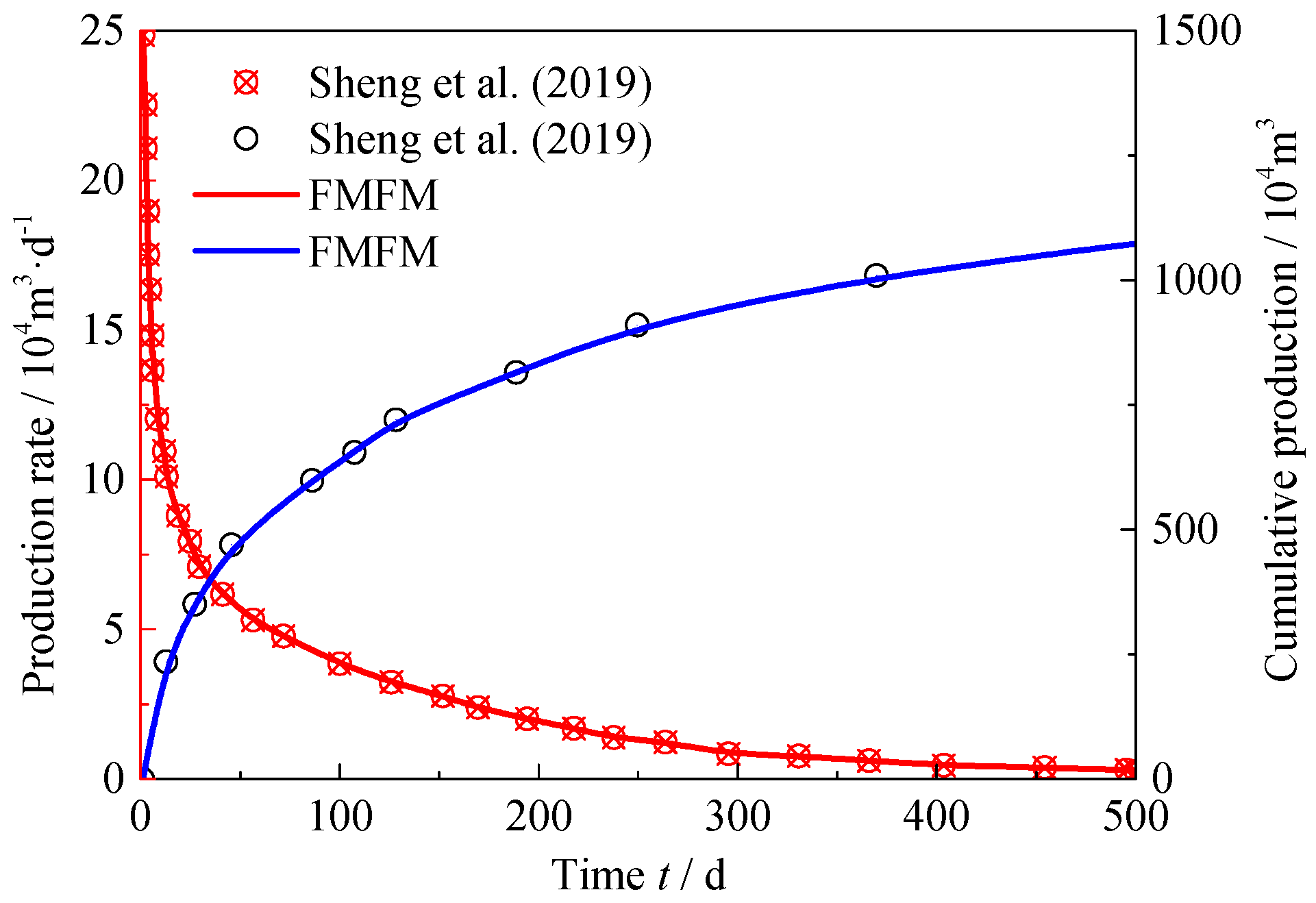
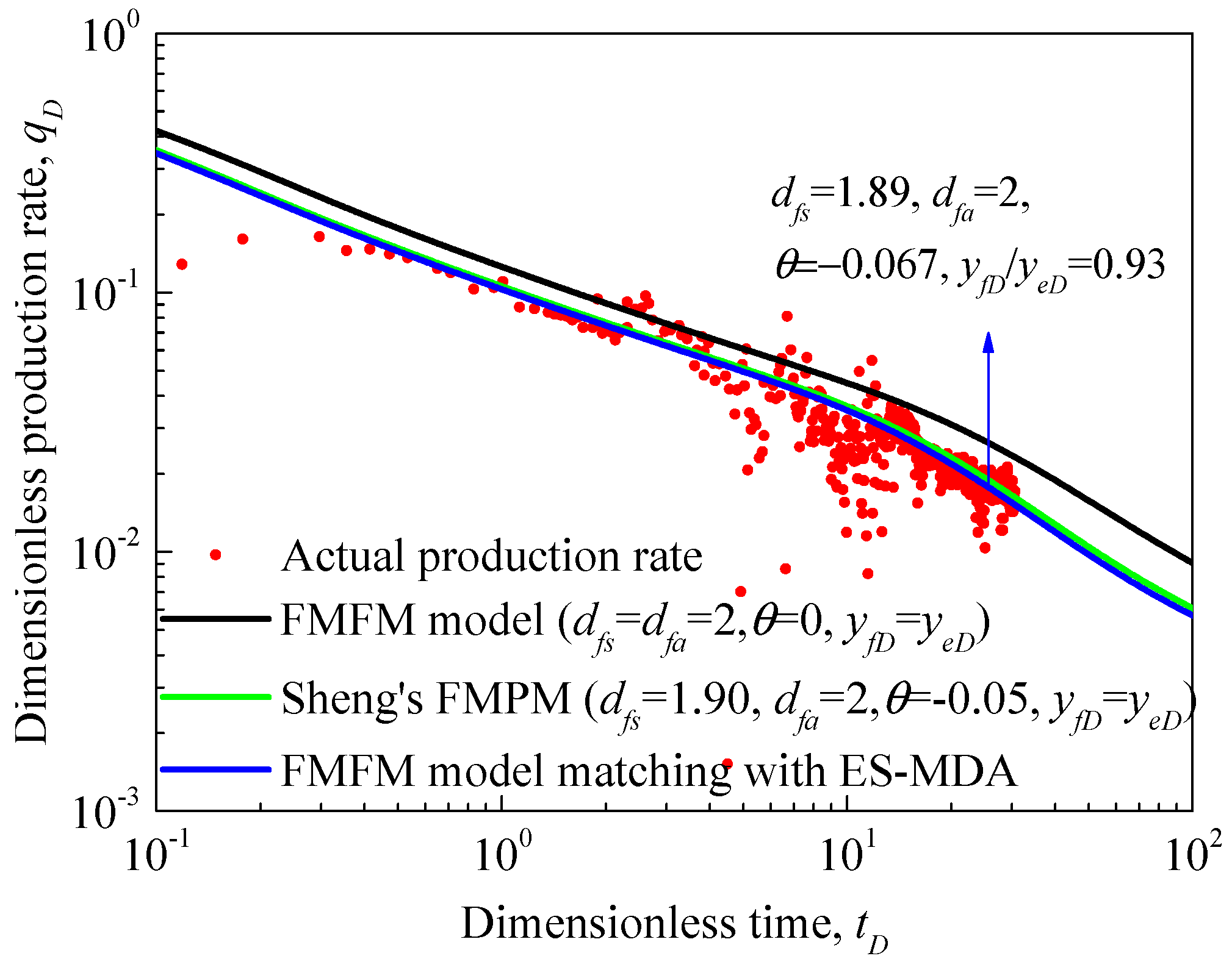
3. Model Verification and Discussion

3.1. Model Verification

The SRV size was assumed to be the same as with the half-length of HF spacing (yf = ye), the presented FMFM model can be simplified as the model proposed by Sheng et al. [20]. The basic parameters used for FMFM and the Sheng’s model are listed in Table 1. The comparison of two models are shown as Figure 4. The results indicate that the production rate and cumulative production calculated by the FMFM presented in this study can fit well with those of Sheng’s model. The classical trilinear flow model can be simplified by FMFM when the SRV size between HFs and the fractal distribution of induced-fracture are not considered. In addition, if the shale gas transport mechanisms are ignored in FMFM, the model can be used to predict the production of MFHWs in tight gas and even in tight oil reservoirs fast.

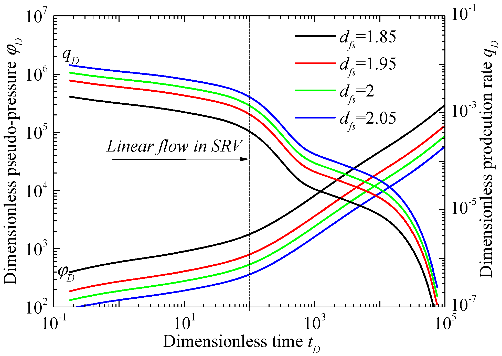
3.2. Sensitivity Analysis of Properties of SRV

Figure 5 and Figure 6 show that the dimensionless pseudo-pressure and dimensionless production rate with different tortuosity index and fractal dimensions of induced-fracture spacing by FMFM, which reflects the various properties of SRV for MFHWs in unconventional gas reservoirs. Figure 5 shows that the dimensionless pseudo-pressure is larger and the dimensionless production rate is smaller when the tortuosity index of induced-fracture θ increases. The larger tortuosity index of induced-fracture θ means the longer flow path of gas transport in SRV. When the tortuosity index of induced-fracture θ is larger than 0, the properties of induced-fracture will decrease far from HF. When the tortuosity index of induced-fracture θ is equal to 0, the properties of induced-fracture is homogeneous in SRV.
Figure 6 indicates that the dimensionless pseudo-pressure is smaller and the dimensionless production rate is larger when the fractal dimension of induced-fracture dfs increases. The larger fractal dimension of induced-fracture dfs leads to a larger equivalent permeability in SRV. In addition, the linear low in SRV can make the WHFWs produce more gas from the formation, which suggests that the induced-fracture system can improve the development effect for unconventional reservoirs.

4. Application of FMFM with ES-MDA Method

4.1. ES-MDA Method

In order to avoid the model update and parameter-state inconsistency, which makes the ensemble Kalman filter (EnKF) complicated, and achieve a better data matching with the ensemble smoother (ES), Emerick and Reynolds [35] reported ES-MDA by assimilating the same observed data multiple times with the covariance matrix of the measurement errors simultaneously. Numerical experiments and examples have shown that the ES-MDA method can provide a better data matching and reduce the uncertainty of model description than the ES method and the EnKF method. Based on the synthetic case and field case data, the application of ES-MDA history matching technology and FMFM for MFHWs is discussed in this section.
The reservoir simulation models are typically stable functions of the rock property fields, which is different with the oceanic and atmospheric models. Based on the common assumption in history-matching problems that the model uncertainty is ignored, we just need to take the parameter-estimation problem into account for ES. Thus, the analyzed vector of model parameters can be given by
m j a = m j + C M D ( C D D + C D ) 1 ( d u c , j d j ) ,   f o r   j = 1 , , N e ,
where C M D is the cross-covariance matrix between the prior vector of model parameters m j and the vector of predicted data d ; C D D is the Nd—dimension auto-covariance matrix of predicted data; Nd is the total number of measurements assimilated; d u c ~ N ( d o b s , C D ) ; d o b s is the Nd—dimensional vector of observed data; C D is the Nd—dimension covariance matrix of observed data measurement errors; and Ne is the number of ensemble member.
Emerick and Reynolds [35] have mentioned that ES-MDA can be used in the nonlinear case because ES is equivalent to a single Gauss–Newton iteration with a full step and an average sensitivity estimated from the prior ensemble, in which case the MDA can be interpreted as an “iterative” ensemble smoother. The ES-MDA algorithm is presented as follows:
(1)
Estimate the number of data assimilations Na, and the coefficients α i ( i = 1 N a 1 α i = 1 ), for i = 1 , , N a .
(2)
For i = 1   t o   N a
  • Run the ensemble from time zero for obtaining the vector of predicted data
    d j = g ( m j ) ,   f o r   j = 1 , , N e ,
    where g ( · ) is the nonlinear forward model, d j is assignment the model parameters to vector m j at time zero.
  • For each ensemble member, perturb the observation vector by
    d u c , j = d o b s + α i C D 1 / 2 z d , j ,   f o r   j = 1 , , N e ,
    where z d , j ~ N ( 0 , Ι N d ) .
  • Update the ensemble
    m j a = m j + C M D ( C D D + α i C D ) 1 ( d u c , j d j ) ,   f o r   j = 1 , , N e ,
    where C = C D D + α i C D [ C D D + α 1 C D C D D C D D C D D + α 2 C D C D D C D D C D D C D D + α N a C D ] ; C M D = 1 N e 1 j = 1 N e ( m j m ¯ ) ( d j d ¯ ) T ; C D D = 1 N e 1 j = 1 N e ( d j d ¯ ) ( d j d ¯ ) T ; m ¯ and d ¯ represent the average values of model parameters and prediction parameter ensembles respectively.
In the procedure of MDA algorithm mentioned above, the data are assimilated Na times continuously, and the ensemble needs to be rerun before each data assimilation. At the same time, in the ES-MDA algorithm, every time the data is assimilated repeatedly, the disturbance observation vector is resampled. The procedure will reduce the sampling problems due to the matching outliers that may occur when the observation data is perturbed.

4.2. Synthetic Case

Based on the simulator Eclipse, the numerical model of a MFHW in the unconventional gas reservoir is established. The numbers of grids are X × Y × Z = 80 × 260 × 3 and the grid steps are X × Y × Z = 5 m × 5 m × 5 m, respectively. A dual-porosity media model is used to describe the SRV (DUALPORO keyword), and a single-porosity medium model is used to describe the USRV. Hydraulic fractures are described by LGR keyword as shown in Figure 7. If only the gas viscous flow with slippage effect is considered, then the FMFM can be simplified as a semianalytic model for a MFHW with the homogeneous SRV in the tight gas reservoir. We set the same modeling parameters of FMFM with those of numerical model and then discuss the applicability of FMFM with ES-MDA.
Firstly, according to the dimensionless parameters listed in Table A1, the production rate of the numerical model can be non-dimensionalized as q D = p q f / ( 2 π k w h c i ( φ φ w f ) ) .
Then, the Nd—dimensional vector of observed data can be chosen as:
d o b s = [ d s T , q o T ] N d × 1 T ,
where ds donates the Nd-dimensional vector of static parameters of the reservoir and MFHW; qo donates the dimensionless production rate of numerical model.
The Nd × Nd covariance matrix of observed data measurement errors is given by
C D = [ σ d 1 2 σ d N d 2 ] N d × N d ,
where σd is equal to 0.3 for real production rate.
The matching results of dimensionless production rate by ES-MDA after 4 iterations and error analysis are shown in Figure 8. The values of some variables are listed as Np = 23, Nd = 115, Ne = 100, and α i = 2. Meanwhile, the root-mean-square error and the average objective function in Figure 7 can be expressed as, respectively,
R M S E = j = 1 N e ( d s o b s d s j ) 2 N p ,
O ( m ) = 1 N d [ g ( m ) d o b s ] T C D 1 [ g ( m ) d o b s ] .
Figure 8 shows that the error between the ensemble mean model and that of true model is large with one iteration, and the distribution range of ensemble members is large. All models of the ensemble (light blue curves) represent the results calculated by FMFM, the ensemble mean (blue curve) represents the calculated results matching with unperturbed observation data (average value of ensemble members), the true value (red curve) is the true dimensionless production rate obtained by FMFM, and the numerical results (red point) is the observed data in Figure 8. We can see that with two iterations, the distribution range of ensemble members becomes small, and ensemble mean model basically coincides with the true model. With three and four iteration, the distribution range of ensemble members is further reduced around the true model, and the ensemble mean model and the observed data are well-matching, which is almost the same with the true model. In addition, the RMSE and objective function values of the prior model are large, indicating that the model errors and data errors are large. After one iteration, the error decreases. The RMSE and objective function values becomes small and basically the same after three and four iterations, which indicates that the matching results are good as shown in Table 2. Therefore, the discussion mentioned above suggests that parameters of FMFM can be obtained by automatically matching production data of the numerical model by ES-MDA method. The technique can also obtain reservoir physical properties and fracturing parameters by matching the actual production data of the oilfield.

4.3. Field Case

The presented FMFM model with ES-MDA history matching method was applied based the shale gas production data of a MFHW in western China [36]. Compared with the presented models based on different simulating conditions, the matching results are shown in Figure 9. Noting that the actual shale gas production rate of a MFHW in western China is represented by red points; when dfs = dfa = 2, θ = 0, yfD = yeD, the FMFM can be assumed as a typical trilinear model with homogenous SRV (black line); the results of Sheng’s FMPM model [20] with fractal SRV are drawn by the light green line, and they calculated the dfs= 1.90 by the box-counting method and the fractal random-fracture-network algorithm and θ = −0.05 by the random walk method; based on the presented FMFM with ES-MDA, the fractal dimensions, tortuosity index, and SRV size can be obtained as shown by the blue line. Figure 9 shows that the fractal dimension and tortuosity index of induced-fracture system matched by FMFM model based on ES-MDA approximate the results of Sheng’s FMPM model. The unmatched early-time data was caused by the early-time flow back process. In addition, the results dimensionless production rate calculated by FMFM were smaller but matched better with actual data than Sheng’s FMPM model when the SRV size was taken into account. This section mainly provides an application case of our presented approach.

5. Conclusions

In this paper, a semianalytic fractal multi-linear flow model (FMFM) for MFHWs in unconventional gas reservoirs with consideration of the heterogeneous distribution of the properties of induced-fracture system is proposed. Fractal dimensions of induced-fracture spacing and aperture and tortuosity index of induced-fracture system are included based on fractal theory to describe the properties of SRV region. For shale gas reservoirs, gas transport mechanisms (viscous flow with slippage, Knudsen diffusion, and surface diffusion) among various medium including porous kerogen, inorganic matter, and fracture system are take into account in FMFM. Then, combining with ES-MDA, the FMFM can be applied not only for prediction of gas production rate for MFHWs in unconventional gas reservoirs but also for main uncertainty parameters matching. Some findings can be drawn as follows:
(1)
The permeability and porosity of the induced-fracture system are affected by the heterogeneous distribution of induced-fractures spacing and aperture. When the fractal dimensions of induced-fracture spacing (dfs) and aperture (dfa) are smaller than 2.0, the permeability of the induced-fracture system decreases with the increase of the distance from HFs in SRV region, which will become increase if dfs > 2.0 or dfa > 2.0. When the tortuosity index of the induced-fracture system θ is larger than 0, the permeability of induced-fracture system also decreases with the increase of the distance from HFs in SRV region.
(2)
The FMFM divides the formation into three types of porous media in shale reservoirs (porous kerogen, inorganic matter, and fracture system). Triple-porosity media and dual-porosity media are used to describe the fractal SRV region and USRV region, respectively. Multiple gas transport mechanisms such as viscous flow with slippage, Knudsen diffusion, and surface diffusion are considered, and gas flow behaviors in different regions are coupled by pseudo-steady cross-flow among various media. The FMFM is verified by other presented model and the results show that the large dfs or small θ causes the small average permeability of the induced-fracture system, which results in large dimensionless pseudo-pressure and small dimensionless production rate.
(3)
Combining the FMFM with ES-MDA history-matching method, the synthetic case for the tight gas reservoir and field case for the shale gas reservoir are discussed. Various main parameters inversions of HFs and NFs are conducted in SRV region. Thus, the presented method can be applied for gas production predicting and history-matching in unconventional gas reservoirs.

Author Contributions

Q.Z. contributed to the conception and drafting the article; S.J. contributed to the study design and manuscript editing. X.W. contributed to programming and analysis; Y.W. contributed to the literature research; Q.M. contributed to the manuscript revision. All authors have read and agreed to the published version of the manuscript.

Funding

This research was funded by the National Natural Science Foundation of China (No.51904279), Fundamental Research Funds for the Central Universities (China University of Geosciences, Wuhan) (No. CUGGC04), and Foundation of Key Laboratory of Tectonics and Petroleum Resources (China University of Geosciences) (No. TPR-2019-03).

Acknowledgments

The authors thank Guanglong Sheng, School of Petroleum Engineering, Yangtze University.

Conflicts of Interest

The authors declare no conflict of interest.

Appendix A. Derivation of Fractal Permeability and Porosity of Induced-Fracture

As shown in Figure 2c, using the fractal theory, the total number of induced-fracture, which is relevant to the fractal dimension of induced-fracture spacing dfs, can be expressed as [37]
0 L x , y n ( L x , y ) d L x , y L x , y d f s ,
where Lx,y is the position of system, m.
Then, Chang and Yortsos [16] presented the expression of the distribution of fracture site as
n ( L x , y ) = α L x , y d f s D ,
where D is the Euclidean dimension, which is equal to 2 in Cartesian coordinate system; α is a constant related to fracture porosity.
For the fracture site, we can obtain
s f ( L x , y ) n ( L x , y ) + b f ( L x , y ) n ( L x , y ) = A S R V ,
where ASRV is the hydraulic fracture half-length, m.
Substituting Equation (A2) into Equation (A3), Equation (A3) can be rewritten as
1 + b f ( L x , y ) s f ( L x , y ) = x f α s f ( L x , y ) L x , y 2 d f s .
In the actual unconventional reservoirs, the value of induced-fracture aperture is commonly far less than that of induced-fracture spacing (bf << sf), and thus Equation (A4) becomes
s f ( L x , y ) | b f ( L x , y ) s f ( L x , y ) 0 = x f α L x , y 2 d f s .
If the induced-fracture spacing at the plane of HF is known, which can be chosen as a reference point, the FFSD in Cartesian coordinate system can be obtained by Equation (A5)
s f ( y ) = s f w ( y y w ) 2 d f s ,
where sfw is the induced-fracture spacing at reference point, m.
For the distribution of induced-fracture aperture (FFAD), the basic form can also be obtained according to Equation (A6) [21]
b f ( y ) = b f w ( y y w ) d f a 2 ,
where bfw is the induced-fracture aperture at reference point, m.
Bai and Elsworth [38] reported the expression of a fracture with a slab shape as
k i f = b f ( y ) 2 12 .
In a representative elementary volume (REV) of fracture network, the fluid flux in the fracture system is given by
v = A r k f ( y ) μ d p d x = n ( y ) A p k i f ( y ) μ d p d L ,
where v is flux of induced-fracture system in a REV, m3/s; μ is the fluid viscosity, Pa·s; and dp is the pressure-difference of a REV in y direction, Pa.
Thus, the fracture permeability and porosity can be obtained as Equations (1) and (2).

Appendix B. Solution for the FMFM Model

For solving the FMFM, the basic dimensionless parameters are defined in Table A1.
Table A1. Basic parameters used in FMFM.
ParametersExpression
Pseudo-pressure for gas phase φ ( p ) = 2 p i p ( p / μ g Z ) d p
Dimensionless pseudo-pressure φ D = 2 π k w h c i ( φ i φ ) / ( p i q f )
Dimensionless time t D = k w t / ( ( ϕ C t ) f m k μ g x f 2 )
Dimensionless length x D = x / x f , y D = y / y w , x e D = x e / x f , y e D = y e / x f , y f D = y f / x f , y w D = y w / x f
Total compressibility coefficient of porous kerogen C t k = C g + ( ε k s c μ s Z R T ) / ( ϕ k ( p L + p k ) 2 )
Transfer coefficient from porous kerogen to inorganic matter λ k = σ k k k x f 2 / k w
Transfer coefficient from inorganic matter to induced-fracture λ m = σ m k m x f 2 / k w
Storage coefficient of porous kerogen ω k = ( ϕ k C t k ) / ( ϕ C t ) f m k
Storage coefficient of inorganic matter ω m = ( ϕ m C g ) / ( ϕ C t ) f m k
Storage coefficient of HFs ω F = ( ϕ F C g ) / ( ϕ C t ) f m k
Subscript i represents the initial conditions; f, m, k represents fracture, inorganic matter, and porous kerogen respectively.
Therefore, transforming the FMFM into Laplace space, the dimensionless forms and solutions for HF, SRV, and USRV can be obtained as follows:
(1)
Dimensionless forms and solutions for USRV.
According to Equations (9) and (10), the dimensionless diffusivity equations in Laplace domain for region III and V can be given by
{ φ 3 k D ¯ = σ k k k x f 2 σ k k k x f 2 + k w s ω k φ 3 m D ¯ ω m s φ 3 m D ¯ = k m k w 2 φ 3 m ¯ x D 2 + σ k k k k w x f 2 ( φ 3 k D ¯ φ 3 m D ¯ ) ,   for   region   III ,
{ φ 5 k D ¯ = σ k k k x f 2 σ k k k x f 2 + k w s ω k φ 5 m D ¯ ω m s φ 5 m D ¯ = k m k w 2 φ 5 m ¯ x D 2 + σ k k k k w x f 2 ( φ 5 k D ¯ φ 5 m D ¯ ) ,   for   region   V .
Solving Equation (A10a,b) with boundary conditions, we can obtain
φ 3 m D ¯ x D | x D = 1 = a 3 ( { K ( 1 / 2 ) ( a 3 x e D ) I ( 1 / 2 ) ( a 3 ) I ( 1 / 2 ) ( a 3 x e D ) K ( 1 / 2 ) ( a 3 ) } { I ( 1 / 2 ) ( a 3 ) K ( 1 / 2 ) ( a 3 x e D ) + I ( 1 / 2 ) ( a 3 x e D ) K ( 1 / 2 ) ( a 3 ) } ) φ f D ¯ | x D = 1 ,
φ 5 m D ¯ x D | x D = 1 = a 5 ( { K ( 1 / 2 ) ( a 5 x e D ) I ( 1 / 2 ) ( a 5 ) I ( 1 / 2 ) ( a 5 x e D ) K ( 1 / 2 ) ( a 5 ) } { I ( 1 / 2 ) ( a 5 ) K ( 1 / 2 ) ( a 5 x e D ) + I ( 1 / 2 ) ( a 5 x e D ) K ( 1 / 2 ) ( a 5 ) } ) φ 4 m D ¯ | x D = 1 ,
where a 3 = a 5 = k w k m ( ω m s + λ k λ k 2 ω k s + λ k ) .
According to Equation (3), the dimensionless diffusivity equations in Laplace domain for region IV can be given by
{ φ 4 k D ¯ = σ k k k x f 2 σ k k k x f 2 + k w s ω k φ 4 m D ¯ ω m s φ 4 m D ¯ = k m k w 1 y w D 2 2 φ 4 m D ¯ y D 2 + σ k k k k w x f 2 ( φ 4 k D ¯ φ 4 m D ¯ ) + k k k w φ 5 m D x D ¯ | x D = 1 .
Solving Equation (A12) with boundary conditions, we can obtain
φ 4 m D ¯ y D | y D = y l D = a 4 ( { K ( 1 / 2 ) ( a 4 y e D ) I ( 1 / 2 ) ( a 4 y l D ) I ( 1 / 2 ) ( a 4 y e D ) K ( 1 / 2 ) ( a 4 y l D ) } { I ( 1 / 2 ) ( a 4 y l D ) K ( 1 / 2 ) ( a 4 y e D ) + I ( 1 / 2 ) ( a 4 y e D ) K ( 1 / 2 ) ( a 4 y l D ) } ) φ f D ¯ | y D = y l D ,
where a 4 = a 5 k w k m y w D 2 a 5 tan h ( ( y l D y e D ) a 5 ) .
(2)
Dimensionless forms and solutions for SRV.
According to Equations (3), (5), and (6), the dimensionless diffusivity equations in Laplace domain for region SRV can be given by
{ ω f s y D θ 2 ( d f a 2 ) φ f D ¯ = 1 y w D 2 2 φ f D ¯ y D 2 + 1 y w D 2 3 ( d f a 2 ) + ( d f s 2 ) θ y D φ f D ¯ y D + y D θ 2 ( d f a 2 ) k m k w φ 3 m ¯ x D | x D = 1 + y D θ 2 ( d f a 2 ) λ m ( φ 2 m D ¯ φ f D ¯ ) φ 2 k D ¯ = λ k λ k + s ω k φ 2 m D ¯ ω m s φ 2 m D ¯ = λ k ( φ 2 k D ¯ φ 2 m D ¯ ) λ m ( φ 2 m D ¯ φ f D ¯ ) .
Solving Equation (A14) with boundary conditions, we can obtain
φ f D ¯ y D | y D = y w D = a 2 y w D 1 + m 1 2 n 1 2 ( I 1 m 1 2 + m 1 n 1 ( 2 a 2 2 + m 1 n 1 y w D 2 + m 1 2 n 1 2 ) h 1 h 2 K 1 m 1 2 + m 1 n 1 ( 2 a 2 2 + m 1 n 1 y w D 2 + m 1 2 n 1 2 ) y w D 1 n 1 2 ( I 1 n 1 2 + m 1 n 1 ( 2 a 2 2 + m 1 n 1 y w D 2 + m 1 2 n 1 2 ) + h 1 h 2 K 1 n 1 2 + m 1 n 1 ( 2 a 2 2 + m 1 n 1 y w D 2 + m 1 2 n 1 2 ) ) ) φ F D ¯ | y D = y w D ,
where a 2 = y w D 2 { ω f s k m k w a 3 ( { K ( 1 2 ) ( a 3 x e D ) I ( 1 2 ) ( a 3 ) I ( 1 2 ) ( a 3 x e D ) K ( 1 2 ) ( a 3 ) } { I ( 1 2 ) ( a 3 ) K ( 1 2 ) ( a 3 x e D ) + I ( 1 2 ) ( a 3 x e D ) K ( 1 2 ) ( a 3 ) } ) + λ m ω m s + λ k ω k s λ k + ω k s ω m s + λ k ω k s λ k + ω k s + λ m } , m 1 = d f a + d f s 4 , n 1 = 3 ( d f a 2 ) + ( d f s 2 ) θ , h 1 = a 2 b 2 y f D m 1 n 1 2 I 1 m 1 2 + m 1 n 1 ( 2 a 2 2 + m 1 n 1 y f D 2 + m 1 2 n 1 2 ) I 1 n 1 2 + m 1 n 1 ( 2 a 2 2 + m 1 n 1 y f D 2 + m 1 2 n 1 2 ) , h 2 = K 1 n 1 2 + m 1 n 1 ( 2 a 2 2 + m 1 n 1 y f D 2 + m 1 2 n 1 2 ) + a 2 b 2 y f D m 1 n 1 2 K 1 m 1 2 + m 1 n 1 ( 2 a 2 2 + m 1 n 1 y f D 2 + m 1 2 n 1 2 ) , b 2 = a 5 ( { K ( 1 / 2 ) ( a 5 x e D ) I ( 1 / 2 ) ( a 5 ) I ( 1 / 2 ) ( a 5 x e D ) K ( 1 / 2 ) ( a 5 ) } { I ( 1 / 2 ) ( a 5 ) K ( 1 / 2 ) ( a 5 x e D ) + I ( 1 / 2 ) ( a 5 x e D ) K ( 1 / 2 ) ( a 5 ) } ) .
(3)
Dimensionless forms and solutions for HFs.
According to Equation (14), the dimensionless diffusivity equations in Laplace domain for HFs can be given by
ω F s φ F D ¯ = k F k w 2 φ F D ¯ x D 2 + x f 2 y w 2 φ F D ¯ y D | y = y w D ,
Solving Equation (A16) with boundary conditions, we can obtain the pseudo-pressure in well bottom-hole in Laplace domain as Equation (16).

References

  1. Yuan, B.; Su, Y.; Moghanloo, R.G.; Rui, Z.; Wang, W.; Shang, Y. A new analytical multi-linear solution for gas flow toward fractured horizontal wells with different fracture intensity. J. Nat. Gas Sci. Eng. 2015, 23, 227–238. [Google Scholar] [CrossRef]
  2. Sheng, G.; Zhao, H.; Su, Y.; Javadpour, F.; Wang, C.; Zhou, Y.; Liu, J.; Wang, H. An analytical model to couple gas storage and transport capacity in organic matter with noncircular pores. Fuel 2020, 268, 117288. [Google Scholar] [CrossRef]
  3. Sheng, G.; Su, Y.; Zhao, H.; Liu, J. A unified apparent porosity/permeability model of organic porous media: Coupling complex pore structure and multi-migration mechanism. Adv. Geo-Energy Res. 2020, 4, 115–125. [Google Scholar] [CrossRef]
  4. Arevalo-Villagran, J.A.; Wattenbarger, R.A.; Samaniego-Verduzco, F.; Pham, T.T. Production analysis of long-term linear flow in tight gas reservoirs: Case histories. In Proceedings of the SPE Annual Technical Conference and Exhibition, Society of Petroleum Engineers, New Orleans, LA, USA, 30 September–3 October 2001. [Google Scholar]
  5. Al Ahmadi, H.A.; Almarzooq, A.M.; Wattenbarger, R.A. Application of linear flow analysis to shale gas wells-field cases. In Proceedings of the SPE Unconventional Gas Conference, Society of Petroleum Engineers, Pittsburgh, PA, USA, 23–25 February 2010. [Google Scholar]
  6. Yu, W. Developments in Modeling and Optimization of Production in Unconventional Oil and Gas Reservoirs. Ph.D. Thesis, The University of Texas at Austin, Austin, TX, USA, 2015. [Google Scholar]
  7. Yao, S.; Wang, X.; Zeng, F.; Li, M.; Ju, N. A composite model for multi-stage fractured horizontal wells in heterogeneous reservoirs. In Proceedings of the SPE Russian Petroleum Technology Conference and Exhibition, Society of Petroleum Engineers, Moscow, Russia, 24–26 October 2016. [Google Scholar]
  8. Ozkan, E.; Brown, M.L.; Raghavan, R.S.; Kazemi, H. Comparison of fractured horizontal-well performance in conventional and unconventional reservoirs. In Proceedings of the SPE Western Regional Meeting, Society of Petroleum Engineers, San Jose, CA, USA, 24–26 March 2009. [Google Scholar]
  9. Brown, M.; Ozkan, E.; Raghavan, R.; Kazemi, H. Practical solutions for pressure-transient responses of fractured horizontal wells in unconventional shale reservoirs. SPE Reserv. Eval. Eng. 2011, 14, 663–676. [Google Scholar] [CrossRef]
  10. Stalgorova, K.; Mattar, L. Analytical model for unconventional multifractured composite systems. SPE Reserv. Eval. Eng. 2013, 16, 246–256. [Google Scholar] [CrossRef]
  11. Wang, W.; Zheng, D.; Sheng, G.; Zhang, Q.; Su, Y. A review of stimulated reservoir volume characterization for multiple fractured horizontal well in unconventional reservoirs. Adv. Geo-Energy Res. 2017, 1, 54–63. [Google Scholar] [CrossRef] [Green Version]
  12. Luo, W.; Tang, C.; Zhou, Y.; Ning, B.; Cai, J. A new semi-analytical method for calculating well productivity near discrete fractures. J. Nat. Gas Sci. Eng. 2018, 57, 216–223. [Google Scholar] [CrossRef]
  13. Cai, J.; Yu, B. Prediction of maximum pore size of porous media based on fractal geometry. Fractals 2010, 18, 417–423. [Google Scholar] [CrossRef]
  14. Yang, F.; Ning, Z.; Liu, H. Fractal characteristics of shales from a shale gas reservoir in the Sichuan Basin, China. Fuel 2014, 115, 378–384. [Google Scholar] [CrossRef]
  15. Sheng, G.; Su, Y.; Wang, W.; Javadpour, F.; Tang, M. Application of fractal geometry in evaluation of effective stimulated reservoir volume in shale gas reservoirs. Fractals 2017, 25, 1740007. [Google Scholar] [CrossRef] [Green Version]
  16. Chang, J.; Yortsos, Y.C. Pressure Transient Analysis of Fractal Reservoirs. SPE Form. Eval. 1990, 5, 31–38. [Google Scholar] [CrossRef]
  17. Cossio, M.; Moridis, G.; Blasingame, T.A. A semianalytic aolution for flow in finite-conductivity vertical fractures by use of fractal theory. SPE J. 2013, 18, 83–96. [Google Scholar] [CrossRef]
  18. Acuna, J.A.; Ershaghi, I.; Yortsos, Y.C. Practical application of fractal pressure transient analysis of naturally fractured reservoirs. SPE Form. Eval. 1995, 10, 173–179. [Google Scholar] [CrossRef]
  19. Wang, W.; Shahvali, M.; Su, Y. A Semi-Analytical Fractal Model for Production from Tight Oil Reservoirs with Hydraulically Fractured Horizontal Wells. Fuel 2015, 158, 612–618. [Google Scholar] [CrossRef]
  20. Sheng, G.; Xu, T.; Gou, F.; Su, Y.; Wang, W.; Lu, M.; Zhan, S. Performance analysis of multi-fractured horizontal wells with complex fracture networks in shale gas reservoirs. J. Porous Media 2019, 22, 299–320. [Google Scholar] [CrossRef]
  21. Sheng, G.; Su, Y.; Wang, W. A new fractal approach for describing induced-fracture porosity/permeability/compressibility in stimulated unconventional reservoirs. J. Pet. Sci. Eng. 2019, 179, 855–866. [Google Scholar] [CrossRef]
  22. Samandarli, O.; Al Ahmadi, H.A.; Wattenbarger, R.A. A semi-analytic method for history matching fractured shale gas reservoirs. In Proceedings of the SPE Western North American Region Meeting, Society of Petroleum Engineers, Anchorage, AK, USA, 7–11 May 2011. [Google Scholar]
  23. Hategan, F.; Hawkes, V.R. Well production performance analysis for unconventional shale gas reservoirs: A conventional approach. In Proceedings of the SPE Canadian Unconventional Resources Conference, Society of Petroleum Engineers, Calgary, AB, Canada, 30 October–1 November 2012. [Google Scholar]
  24. Cho, Y.; Ozkan, E.; Apaydin, O.G. Pressure-dependent natural-fracture permeability in shale and its effect on shale-gas well production. SPE Reserv. Eval. Eng. 2013, 16, 216–228. [Google Scholar] [CrossRef]
  25. Ogunyomi, B.A.; Patzek, T.W.; Lake, L.W.; Kabir, C.S. History matching and rate forecasting in unconventional oil reservoirs using an approximate analytical solution to the double porosity model. In Proceedings of the SPE Eastern Regional Meeting, Society of Petroleum Engineers, Charleston, WV, USA, 21–23 October 2014. [Google Scholar]
  26. Clarkson, C.R.; Williams-Kovacs, J.D.; Qanbari, F.; Behmanesh, H.; Sureshjani, M.H. History-matching and forecasting tight/shale gas condensate wells using combined analytical, semi-analytical, and empirical methods. J. Nat. Gas Sci. Eng. 2015, 26, 1620–1647. [Google Scholar] [CrossRef]
  27. Nobakht, M.; Mattar, L. Analyzing production data from unconventional gas reservoirs with linear flow and apparent skin. J. Can. Pet. Technol. 2012, 51, 52–59. [Google Scholar] [CrossRef]
  28. Chen, Z.M.; Liao, X.W.; Zhao, X.L.; Liu, H.M.; Tian, J.; Zhu, L.T.; Wang, L.; Zhao, H.J. A comprehensive model for performance forecast of multiple fractured horizontal well in unconventional reservoirs: A case study. In Proceedings of the SPE Trinidad and Tobago Section Energy Resources Conference, Society of Petroleum Engineers, Port of Spain, Trinidad and Tobago, 13–15 June 2016. [Google Scholar]
  29. Warren, J.R.; Root, P.J. The behavior of naturally fractured reservoirs. Soc. Pet. Eng. 1963, 3, 245–255. [Google Scholar] [CrossRef] [Green Version]
  30. Bour, O.; Davy, P. On the connectivity of three-dimensional fault networks. Water Resour. Res. 1998, 34, 2611–2622. [Google Scholar] [CrossRef]
  31. Zhang, Q.; Su, Y.; Zhao, H.; Wang, W.; Zhang, K.; Lu, M. Analytic evaluation method of fractal effective stimulated reservoir volume for fractured wells in unconventional gas reservoirs. Fractals 2018, 26, 1850097. [Google Scholar] [CrossRef]
  32. Fan, D.; Ettehadtavakkol, A. Semi-Analytical Modeling of Shale Gas Flow through Fractal Induced Fracture Networks with Microseismic Data. Fuel 2017, 193, 444–459. [Google Scholar] [CrossRef]
  33. Mukherjee, H.; Economides, M.J. A parametric comparison of horizontal and vertical well performance. SPE Form. Eval. 1990, 6, 209–216. [Google Scholar] [CrossRef]
  34. Van Everdingen, A.F.; Hurst, W. The Application of the Laplace Transformation to Flow Problems in Reservoirs. J. Pet. Technol. 1949, 1, 305–324. [Google Scholar] [CrossRef]
  35. Emerick, A.A.; Reynolds, A.C. Investigation of the sampling performance of ensemble-based methods with a simple reservoir model. Comput. Geosci. 2013, 17, 325–350. [Google Scholar] [CrossRef]
  36. Xu, J.; Guo, C.; Wei, M. Production performance analysis for composite shale gas reservoir considering multiple transport mechanisms. J. Nat. Gas Sci. Eng. 2015, 26, 382–395. [Google Scholar] [CrossRef]
  37. O’Shaughnessy, B.; Procaccia, I. Analytical solutions for diffusion on fractal objects. Phys. Rev. Lett. 1985, 54, 455–458. [Google Scholar] [CrossRef]
  38. Bai, M.; Elsworth, D. Modeling of subsidence and stress-dependent hydraulic conductivity for intact and fractured porous media. Rock Mech. Rock Eng. 1994, 27, 209–234. [Google Scholar] [CrossRef]
Figure 1. Simplified physical model and three typical presented linear-flow models for a multi-fractured horizontal wells (MFHW) in unconventional reservoirs.
Energies 13 03718 g001
Figure 2. Development of physical and mathematical models. (a) Map of micro-seismic monitoring results; (b) simplified physical model presented in this study; (c) multi-linear mathematical model presented in this study (modified from Sheng et al. [20]); (d) idealized homogeneous dual-media model (IDMM) for stimulated reservoir volume (SRV) (modified from Warren and Root [29]); and (e) fractal heterogeneous dual-media model (FDMM) for SRV.
Energies 13 03718 g002
Figure 3. Fracture permeability distribution with different fractal dimensions of induced-fracture spacing and aperture (dfs and dfa) and tortuosity index of induced-fracture (θ). (a) Fracture permeability distribution in SRV with different values of dfs when dfa = 2 and θ = 0; (b) fracture permeability distribution in SRV with different values of dfa when dfs = 2 and θ = 0; and (c) fracture permeability distribution in SRV with different values of θ when dfs = 2 and dfa = 2.
Energies 13 03718 g003
Figure 4. Comparison of production rate and cumulative production between FMFM and Sheng’s model [20].
Energies 13 03718 g004
Figure 5. Comparison of production rate and pseudo-pressure with different tortuosity index of induced-fracture θ by FMFM (dfs = 2 and dfa = 2).
Energies 13 03718 g005
Figure 6. Comparison of production rate and pseudo-pressure with different fractal dimension of induced-fracture spacing dfs by FMFM (dfa = 2 and θ = −0.05).
Energies 13 03718 g006
Figure 7. Schematic diagram of a MFHW numerical model (yl = ye).
Energies 13 03718 g007
Figure 8. The matching results of dimensionless production rate by ensemble smoother with multiple data assimilation (ES-MDA) after 4 iterations and error analysis.
Energies 13 03718 g008
Figure 9. The matching results of actual shale gas production rate and different models.
Energies 13 03718 g009
Table 1. Parameters used in multi-linear flow model (FMFM) and Sheng’s model [20].
ParametersValueParametersValue
Fractal dimension of induced-fracture spacing, dfs1.95Pore size in porous kerogen, rk (m)10 × 10−9
Fractal dimension of induced-fracture aperture, dfa2.0Portion of kerogen volume, εks0.5
Tortuosity index of induced-fracture, θ−0.05Porous kerogen porosity, ϕk0.1
Porosity of induced-fracture, ϕ f 10−4Porous kerogen tortuosity, τk5
HF half-spacing, ye (m)100Langmuir pressure, pL (MPa)13.78
HF half-length, xf (m)50Gas viscosity, μg (mPa·s)0.0184
HF permeability, kF (m2)103 × 10−15Gas compressibility, Cg (MPa−1)5 × 10⁻²
HF half-width, yw (m)0.01Surface diffusion coefficient, Ds (m2/s)1 × 10−5
HF porosity, ϕF10−3Molecular mass of shale gas, M (kg/mol)0.016
Total compressibility of the inorganic matter, Ctm (MPa−1)7.5 × 10⁻³Langmuir volume on kerogen surface, cμs (mol/m3)700
Total compressibility of induced-fracture, Ctf (MPa−1)4 × 10⁻³Fraction of molecules striking pore wall which are diffusely reflected, f0.8
Inorganic matter porosity, ϕm0.1Total compressibility of the porous kerogen, Ctk (MPa−1)7.5 × 10⁻³
Inorganic matter tortuosity, τm5Reservoir thickness, h (m)19
Induced-fracture permeability at yw, kw (m2)2 × 10⁻¹⁵Initial pressure, pi (MPa)17
Pore size in inorganic matter, rm (m)20 × 10−9Well bottom pressure, pwf (MPa)12
Formation temperature, T (K)338Reservoir half-width, xe (m)200
Table 2. Comparison of matching results of FMFM and numerical model parameters by ES-MDA.
ParametersEclipseFMFMParametersEclipseFMFM
Total compressibility coefficient, MPa−15.5 × 10−35.2714 × 10−3USRV matrix permeability, m21 × 10−190.887 × 10⁻¹⁸
HF permeability, m215 × 10−137.82 × 10⁻¹³Induced-fracture permeability, m21 × 10−161.33 × 10⁻¹⁶
SRV matrix permeability, m21 × 10−180.77 × 10⁻¹⁸Other parametersEqual values

