Forecasts of Value-at-Risk and Expected Shortfall in the Crude Oil Market: A Wavelet-Based Semiparametric Approach

Abstract

We propose the use of wavelet-based semiparametric models for forecasting the value-at-risk (VaR) and expected shortfall (ES) in the crude oil market. We compared the forecast outcomes across different time scales for three semiparametric models, three nonparametric, distribution-based, generalized, autoregressive, conditional, heteroskedasticity (GARCH) models, and three rolling-window models. We found that the GARCH model estimated by the Fissler and Ziegel (FZ) zero loss minimization (GARCH-FZ) model performs the best at forecasting the VaR and ES in the short term, whereas the hybrid model performs the best for mid- and long-term time scales. Thus, long-term investors should consider the hybrid model and short-term investors should employ the GARCH-FZ model in their risk management processes. Overall, our proposed wavelet-based semiparametric models outperform the other models tested for all time scales and market conditions. As such, we suggest that these models are considered for the management of crude oil price risk and in the development of energy policy.

1. Introduction

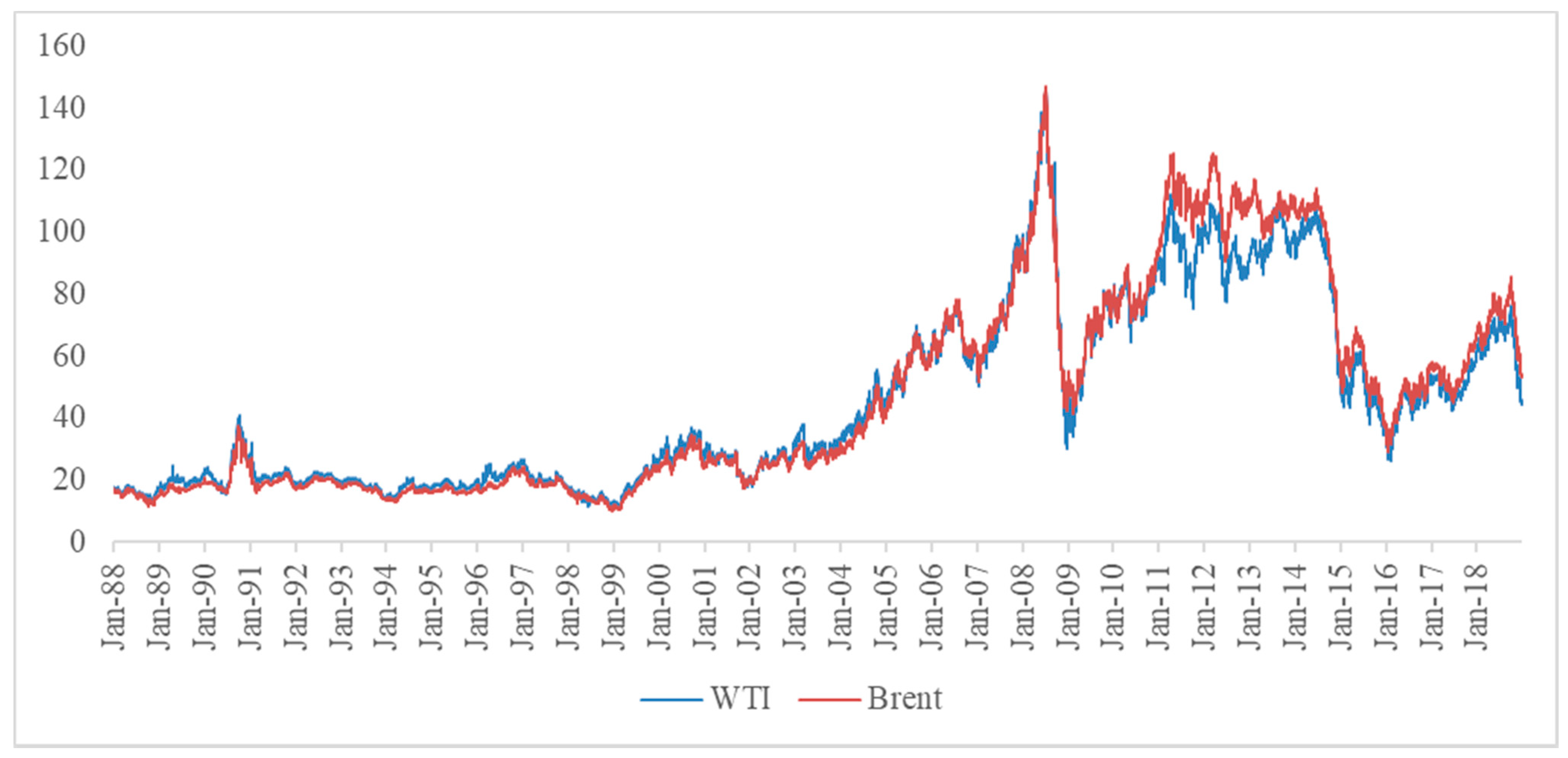
Crude oil is one of the most volatile financial assets and important industrial inputs in the global economy. As such, the crude oil risk has been well researched. From an economic perspective, a highly volatile crude oil price can cause great economic uncertainty, as was the case during the great recession due to the sharp increase in crude oil prices. Then, during the 2008 global financial crisis, the sharp decline in crude oil spot prices caused great uncertainty in the financial market. For example, the average annualized standard deviation of the West Texas Intermediate (WTI) crude oil price in our sample period is 39.186, whereas that of the S&P 500 market index is 12.873. (This ratio is based on the authors’ own calculations using the sample period of the present study.) In other words, the volatility of crude oil is three times that of the U.S. stock market.

Given this high volatility, managing and forecasting the risk associated with the crude oil market has become increasingly important. For investors, the high level of risk causes extreme price movements, which can damage their portfolios [1]. For policymakers, the highly volatile crude oil market makes the future state of the economy less certain, thus making it more difficult to formulate appropriate policies. Therefore, the main goal of this study was to develop an alternative approach to forecast the crude oil risk, especially in cases of extreme risk over time, thus helping investors and policymakers to quantify such risk.

Furthermore, the value-at-risk (VaR) measure is widely used by financial intermediaries and banks to quantify the market risk [2]. However, this measure fails to capture extreme tail events, which occur frequently in the crude oil market. Therefore, we employed the expected shortfall (ES) measure to assess extreme risk in this market. Since the Basel III requirements are implemented worldwide, risk managers, banking supervisors, and regulators tend to pay greater attention to ES measures. Therefore, it is important that we measure extreme risk in the crude oil market by considering both the VaR and the ES.

In prior studies, the accuracy of VaR and ES forecasts depended heavily on having relevant volatility estimation and conditional distribution specifications [3,4,5,6,7,8,9,10,11]. On one hand, volatility estimation depends on an investor’s time horizon, where losses are potentially greater in the short run than they are in the long run. For example, by incorporating a wavelet analysis into the capital asset pricing model (CAPM), Fernandez [7] showed that volatility increases with the data frequency. Similarly, Cifter [5] showed improved financial risk forecasting by using the wavelet-based extreme value theory. Specifically, since investors are sensitive to the investment horizon, incorporating wavelet analysis will provide investors with a good indicator to evaluate their portfolio risk across the investment horizon. Meanwhile, policymakers focus more on the long-term effect of crude oil risk on the economy, which can be examined using the empirical results from wavelet analysis.

On the other hand, focusing on model selection may mean that assumptions are made and that a distribution needs to be selected. For example, Lyu et al. [10] examined three distributions (i.e., skewed general error, generalized asymmetric Student’s t, and generalized hyperbolic skewed Student’s t) and showed that a more accurate VaR measurement could be estimated. Instead of choosing an optimal distribution, Zhao et al. [11] employed fractional generalized autoregressive conditional heteroskedasticity (GARCH) models to perform a VaR forecast, in which they considered long memory, volatility clustering, asymmetry, and thick tails. In their results, the fractionally integrated, asymmetric power, autoregressive, conditional heteroscedasticity in mean with extreme value theory (FIAPARCH-M-EVT) model performed the most effectively. In other words, the parameters estimated using a nonparametric model change with the distribution and assumptions, implying that the distribution with the best fit is unstable across sample periods (e.g., [8]).

However, as a coherent risk measure, the ES has no loss function to minimize the expected loss, which also means that we cannot compare the results [12]. To resolve this problem, we employed the semiparametric approach of Fissler and Ziegel (FZ) [13] and added a wavelet approach to the ES and VaR (wavelet-based semiparametric approaches also exist; see Boubaker and Sghaier [14] and Zhou and Lin [15]). Specifically, we based our VaR and ES semiparametric models on the generalized autoregressive score (GAS) model [16], which is quite different from the wavelet decomposed nonlinear ensemble VaR model [17]. In other words, our proposed models can be elicited from the loss function and are irrelevant to the conditional distribution under different time scales.

Therefore, the contributions of this study are as follows: firstly, we enrich the current literature by considering an ES measure to model extreme risk in the crude oil market using different time scales. We chose the ES measure because the crude oil market exhibits extreme price movements in our sample compared to those of the VaR measure, which does not adequately account for the extreme tail risk. Moreover, by combining the wavelet and semiparametric approaches, we examined the dynamics of forecasts based on both the ES and the VaR measures over time (particularly in the long term). Additionally, we considered potential performance gains across time scales by introducing a wavelet analysis into the risk modeling process.

Secondly, we addressed the problem of elicitability in the ES measure and removed doubts about its backtestability [18,19]. Unlike the conditional autoregressive VaR (CAViaR) dynamics [20,21,22], our proposed models are free of backtestability, which means that we cannot compare different risk estimation procedures. Specifically, we employed the FZ loss function to compare the VaR and ES measures based on a parametric or semiparametric model. In addition, we compared the forecast accuracy between the semiparametric GAS model and the nonparametric GARCH model using tests developed by Diebold and Mariano [23]. We also employed goodness-of-fit procedures to justify the model.

Thirdly, we propose a semiparametric GAS model to jointly measure the VaR and ES in the crude oil market. By doing so, we remove the need to make assumptions or select distributions. Unlike the direct approach of FZ [13], Taylor [24] estimated the dynamic VaR and ES measures jointly using an alternative distribution, such as the asymmetric Laplace distribution, and this has been proven to be effective under loss functions [13]. In contrast to other studies that rely heavily on distribution and model selection (e.g., [8,10]), our results show that the semiparametric model provides better forecasting results and robustness. In summary, our results provide new insights into market risk predictions for the crude oil market over different time scales.

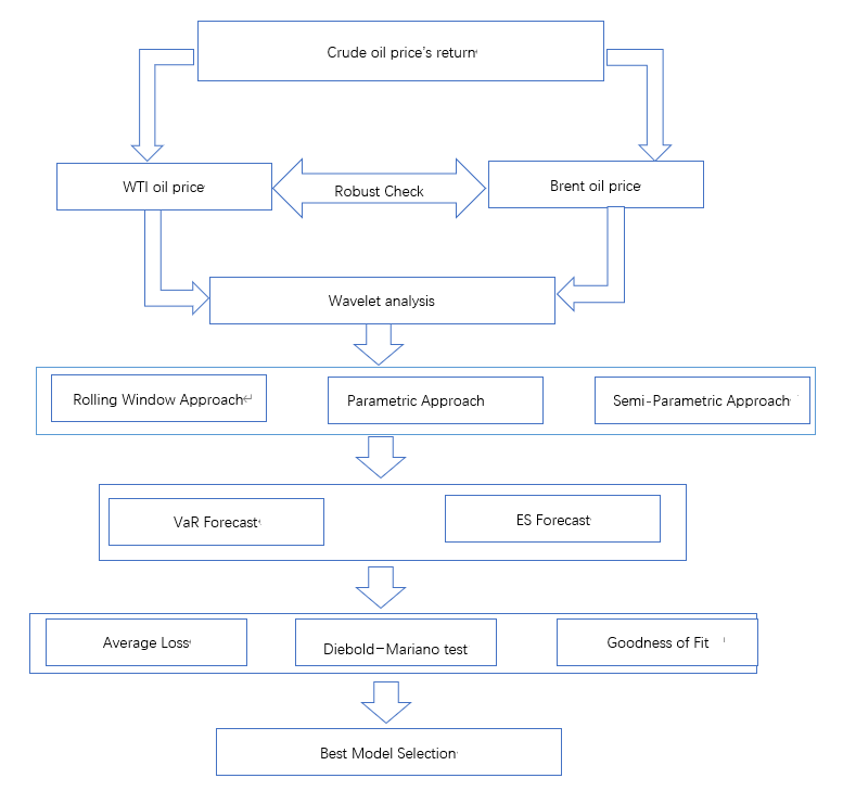
The remainder of this paper proceeds as follows: in Section 2, we present the wavelet, rolling-window, nonparametric-based, and semiparametric models, which we used to forecast the VaR and ES, along with their estimation methodologies. In Section 3, we present the data and the descriptive statistics. In Section 4, we summarize the in-sample estimates and the out-of-sample forecasts and compare the measurements and robustness of each. We conclude the paper in Section 5.

2. Methodology

2.1. Dynamic VaR and ES Models

Various dynamic ES and VaR measures exist to estimate the VaR and ES, the simplest of which is the rolling-window approach, based on the following quantities:

$$\widehat{Va{R}_t}=\widehat{Quantile}{\left\{Y_t\right\}}_{s=t-m}^{t-1},\widehat{E{S}_t}=\frac{1}{\alpha m}{\sum }_{s=t-m}^{t-1}{Y}_t\mathbf{1}\{Y_t\le \widehat{Va{R}_t}\},$$

(1)

where $Y_t$ denotes the crude oil returns over the sample period t; hence, $\widehat{Quantile}{\left\{Y_t\right\}}_{s=t-m}^{t-1}$ denotes the sample quantile of $Y_t$ from t−m to t−1 over period s, and $m$ denotes the window size. In general, $m$ is set to 125, 250, or 500 days. In this study, we employed the rolling-window approach as our benchmark model.

2.2. Wavelet Approach

In addition to the rolling window approach, we employed the wavelet transform approach to analyze the dynamic VaR and ES values over different time scales. Wavelet analyses have been widely employed to deconstruct returns in series by period. In particular, we followed the methods of Percival and Walden [25] and Yang et al. [26], employing the maximal overlap discrete wavelet transform (MODWT) to obtain information components across different time scales by decomposing the original series. As a modified version, the MODWT has a similar length and shift invariance to those of the discrete wavelet transform (DWT).

We decomposed the daily crude oil return series $Y=\left\{Y_t,t=1,2,\dots ,N\right\}$ into J frequencies. Then, by combining the MODWT wavelet and scaling filters, we obtained each J frequency’s wavelet coefficients by filtering $Y$ in a circular manner, as follows:

$${\tilde{W}}_{j,t}={\sum }_{l=0}^{L_j-1}{\tilde{h}}_{j,l}{Y}_{t-l mod N}$$

(2)

and

$${\tilde{V}}_{j,t}={\sum }_{l=0}^{L_j-1}{\tilde{g}}_{j,l}{Y}_{t-l mod N},$$

(3)

where ${\tilde{h}}_{j,l}$ denotes the jth-level MODWT wavelet, and ${\tilde{g}}_{j,l}$ denotes a scaling filter of width $L_j=\left(2^j-1\right)\left(L-1\right)+1$. To maximize the number of boundary-free coefficients, we employed the Haar filter to implement the MODWT for out-of-sample forecasts. (We applied the Haar filter mainly because it is reversible, in contrast to other wavelets. By doing so, we were able to make our empirical results more robust by considering data of different frequencies.) For example, ${\tilde{h}}_{1,0}=\frac{1}{2}$, ${\tilde{h}}_{1,1}=-\frac{1}{2}, {\tilde{g}}_{1,0}=\frac{1}{2}$, and ${\tilde{g}}_{1,1}=\frac{1}{2}$ in the initial step. Therefore, ${\tilde{g}}_{j,l}$ measures the localized moving average, and ${\tilde{h}}_{j,l}$ measures the deviations from this average.

We used the matrix notation, as shown by Percival and Walden [25]:

$${\tilde{W}}_J={\tilde{\omega }}_{j}Y$$

(4)

and

$${\tilde{V}}_J={\tilde{\upsilon }}_{j}Y,$$

(5)

where ${\tilde{\omega }}_j$ and ${\tilde{\upsilon }}_j$ represent $N\times N$ matrices, with elements of circularly shifted ${\tilde{h}}_{j,l}$ and ${\tilde{g}}_{j,l}$, respectively. To avoid seasonality in the crude oil return series, we used a multi-resolution analysis (MRA) in the DWT. Then, we expressed the crude oil return series as the sum of the smoothed version of the deconstruction and all coefficients, in matrix form:

$$Y_t={\tilde{S}}_{J,t}+{\sum }_{j=1}^J{\tilde{D}}_{j,t},$$

(6)

where the wavelet detail coefficients at level j are described by ${\tilde{D}}_{j,t}={\tilde{\omega }}_{j,t}^T{\tilde{W}}_{J,t}$, and the smooth coefficients are described by ${\tilde{S}}_{J,t}={\tilde{v}}_{j,t}^T{\tilde{V}}_{J,t}$. Specifically, ${\tilde{D}}_{j,t}$ captures the variance of the crude oil return series at different levels of j, whereas ${\tilde{S}}_{J,t}$ denotes the smooth part of the crude oil return series. Importantly, we rescaled the wavelet and scaling coefficients to retain the variance-preserving property of the DWT. Moreover, because we applied zero-phase filters for the detailed and smooth components, the features in the crude oil return series for any sample size could be correlated with those of the MODWT-based MRA.

As prior empirical studies suggest, crude oil data have a multi-scale, nonlinear, chaotic nature, which breaks the strict assumptions of the parametric model [27,28,29]. At the same time, the assumptions of the distribution are time- and location-invariant, which means that the nonparametric model results differ from the actual results in practice. By combining nonparametric techniques with parametric approaches, we compromised by using the semiparametric model to strike a balance between relaxing the strict assumptions and improving the estimation efficiency. Indeed, prior studies have discussed and explored the linkages between wavelet analyses and extreme value theory [5,17]. In the following sections, we discuss these two approaches in detail.

2.3. Nonparametric Models

For the second type of dynamic model, we modeled the crude oil returns process using a GARCH model, by incorporating a wavelet analysis. Specifically, we employed the autoregressive moving average (ARMA) (p, q) process to model the mean equation for both the original crude oil returns ($Y_t$) and their wavelet details (${\tilde{D}}_{j,t}$), which we can specify as the following:

$$R_t={\varphi }_0+{\sum }_{i=1}^p{\phi }_i{R}_{t-i}+{\sum }_{i=1}^p{\theta }_i{\epsilon }_{t-i}+{\epsilon }_t,$$

(7)

where ${\phi }_i$ and ${\theta }_i$ denote the autoregressive parameter and the moving average parameter, respectively, ${\epsilon }_t$ is the white noise error term, ${\varphi }_0$ is the conditional mean, and $R_t$ is a simplified notation representing both the original crude oil return series ($Y_t$) and its wavelet detail series (${\tilde{D}}_{j,t}$). The optimal p- and q-values were selected based on the Bayesian information criterion (BIC). Following Bollerslev [30], we used the standard GARCH(1, 1) process to model the daily volatility in risk measurement forecasting:

$${\sigma }_t^2=\omega +\gamma {\epsilon }_{t-1}^2+\beta {\sigma }_{t-1}^2,$$

(8)

where $\beta$ denotes the persistence parameter. In particular, we used three common types of distribution: the normal distribution, the skew-t distribution [31], and an empirical distribution.

$$z_t~ iid N\left(0,1\right),z_t~ iid Skew t\left(0,1, v,\lambda \right).$$

(9)

The latter distribution is an empirical distribution function based on a filtered historical simulation [20]. Following Equation (1), we were able to specify the VaR and ES as risk measures for a given time horizon, as follows:

$$Va{R}_t^{\alpha }=F_t^{-1}\left(\alpha \right),E{S}_t^{\alpha }=E(R_t|\left(R_t\le Va{R}_t^{\alpha }\right),F_{t-1}),R_t|F_{t-1}~F_t,$$

(10)

where $z_{\alpha }$ is the left-tailed quantile at value $\alpha =0.05$. The conditional distribution $F_t$ is based on $R_t$.

2.4. Semiparametric Models

Furthermore, we employed the GAS model proposed by Creal et al. [16] and Yuan and Yang [32] to update the current value of the variable from its lagged information. We considered three dynamic models for the comparison. Moreover, to better compare our forecasting results, we only considered the parameter structure with a single variable, because volatility can serve as a useful time-varying risk measure in risk forecasting. The first model is the one-factor GAS model driven by a single variable, ${\kappa }_t$:

$${\varphi }_t=aexp\left\{{\kappa }_t\right\}, e_t=bexp\left\{{\kappa }_t\right\},\mathrm{where} b<a<0,$$

(11)

where ${\varphi }_t$ denotes VaR_t, and $e_t$ denotes ES_t. Following Creal et al. [16] and Patton et al. [33], we were able to specify the evolution equation using the FZ loss function, as follows:

$${\kappa }_t=\omega +\beta {\kappa }_{t-1}+\gamma \frac{1}{e_{t-1}}\left(\frac{1}{\alpha }\mathbf{1}\left\{R_{t-1}\le {\varphi }_{t-1}\right\}{R}_{t-1}-e_{t-1}\right),$$

(12)

where the FZ loss function only identifies ${\varphi }_t$ and $e_t$, whereas the generalized autoregressive process determines the parameters $\omega$, $\beta$, and $\gamma$. For simple identification, we set $\omega$ to zero.

The second model that was used was the GARCH model with FZ loss minimization. Importantly, if the true conditional distribution is known, then the ARMA−GARCH model performs best. Otherwise, the model’s performance can be improved by estimating its parameters using FZ loss minimization. Similarly to Equation (7), $R_t$ is the product of the conditional deviation ${\sigma }_t$ and the parameter distribution ${\eta }_t$, where ${\sigma }_t$ follows the GARCH process and ${\eta }_t\sim iid{F}_{\eta }\left(0,1\right)$. We obtained an analogous structure to the one-factor GAS model and were able to write the dynamic VaR and ES as the following:

$${\varphi }_t=a{\sigma }_t, e_t=b{\sigma }_t,\mathrm{where} a=F_{\eta }^{-1}\left(\alpha \right), b=\mathbb{E}[\eta |\eta <a],.$$

(13)

$${\sigma }_t^2=\omega +\gamma R_{t-1}^2+\beta {\sigma }_{t-1}^2$$

(14)

Therefore, we only needed to estimate the parameter vectors ($\beta$,$\gamma$, a, and b). This approach allowed us to obtain VaR and ES forecasts, rather than volatility forecasts, with the best fit.

The final model was a direct combination of the GAS and GARCH models, which we refer to as the hybrid model, specified as follows:

$$R_t=exp\left\{{\kappa }_t\right\}{\eta }_t, {\eta }_t\sim iid F_{\eta }\left(0,1\right)$$

(15)

$${\kappa }_t=\omega +\beta {\kappa }_{t-1}+\gamma \frac{1}{e_{t-1}}\left(\frac{1}{\alpha }1\left\{R_{t-1}\le {\varphi }_{t-1}\right\}{R}_{t-1}-e_{t-1}\right)+\log R_{t-1}|,$$

(16)

where the latent variable ${\kappa }_t$ is the log of volatility. To ensure that the units remain stable in the evolution equation, we used the lagged log absolute return instead of the lagged squared return. Five parameters ($\beta$,$\gamma$, $\delta$, a, and b) must be estimated in this model.

2.5. Estimation Methodology

In this section, we describe the estimation of the dynamic VaR and ES measures following the FZ approach [13]. Indexed by the functions G₁ and G₂, the scoring function proposed by FZ [13] is consistent for VaR and ES; thus, we used this to address the issue of non-elicitability in the ES measure. Based on these loss functions, the scoring functions provide the true VaR and ES values only by minimizing the expected loss; hence, we were able to construct the following FZ loss functions:

$$L_{FZ}\left(R,\varphi ,e;\alpha ,G_1,G_2\right)=\left(\mathbf{1}\left\{R\le \varphi \right\}-\alpha \right)\left(G_1\left(\varphi \right)-G_1\left(R\right)+\frac{1}{\alpha }{G}_2\left(e\right)\varphi \right)$$

$$-G_2\left(e\right)\left(\frac{1}{\alpha }\mathbf{1}\left\{R\le \varphi \right\}R-e\right)-{ℊ}_2\left(e\right),$$

(17)

where G₁ is increasing, G₂ is increasing and positive, and we have ${ℊ}_{2 }^{\prime }$= G₂. The VaR and ES were derived by minimizing any member of the class:

$$\left(Va{R}_t, E{S}_t\right)=arg\underset{\left(\varphi ,e\right)}{\mathit{min}}{\mathbb{E}}_{t-1}\left[L_{FZ}\left(Y,\varphi ,e;\alpha ,G_1,G_2\right)\right].$$

(18)

To obtain the minimized value of Equation (17), we selected G₁ and G₂ under the FZ loss function. We first defined the loss difference for the two forecasts (${\varphi }_{1,t},e_{1,t}$) and (${\varphi }_{2,t},e_{2,t}$) as $\Delta L_{FZ}\left(R,{\varphi }_{1,t},e_{1,t},{\varphi }_{2,t},e_{2,t}\right)=L_{FZ}\left(Y,{\varphi }_{1,t},e_{1,t}\right)-L_{FZ}\left(Y,e_{1,t},e_{2,t}\right)$. Following Patton and Sheppard [34] and Patton et al. [33], we chose G₁ and G₂ based on the loss function that generates $\Delta L_{FZ}$, which is homogeneous to degree zero.

After identifying the uniqueness of the FZ zero (FZ0) loss minimization loss function, we propose the semiparametric dynamic ES and VaR measures:

$$\left(Va{R}_t, E{S}_t\right)=\left(\varphi \left({\mathit{X}}_{\mathit{t}\mathit{-}\mathbf{1}}\mathit{;}\mathit{\theta }\right),e\left({\mathit{X}}_{\mathit{t}\mathit{-}\mathbf{1}}\mathit{;}\mathit{\theta }\right)\right),$$

(19)

where the information set ${\mathit{X}}_{\mathit{t}\mathbf{-}\mathbf{1}}\in {\mathit{ℱ}}_{\mathit{t}\mathbf{-}\mathbf{1}}$ contains the elements of the specified parametric functions for the true VaR and ES. We estimated the model parameters using the following:

$$\left(Va{R}_t, E{S}_t\right)=arg\underset{\left(\varphi ,e\right)}{\mathit{min}}{\mathbb{E}}_{t-1}\left[L_{FZ}\left(Y,\varphi ,e;\alpha ,G_1,G_2\right)\right].$$

(20)

As Patton et al. [33] suggested, the asymptotic theory estimates $\mathit{\theta }$ effectively in both linear and nonlinear models. Although Equation (12) imposes parametric structures on the lagged information, the dynamic VaR and ES in Equation (1) are free of regularity conditions and assumptions on the conditional distribution. In other words, these models are semiparametric and thus can be used in comparisons with the nonparametric models detailed in Section 2.3.

2.6. Goodness-of-Fit Test

To identify the performance of the VaR and ES measures for the different types of models, we considered a goodness-of-fit test for the out-of-sample forecasts. Given the correct specifications for the VaR and ES measures, this is as follows:

$${\mathbb{E}}_{t-1}\left[\begin{array}{c}\partial L_{FZ}\left(R_t,{\varphi }_t,e_t;\alpha \right)/ \partial {\varphi }_t \\ \partial L_{FZ}\left(R_t,{\varphi }_t,e_t;\alpha \right)/ \partial e_t \end{array}\right]={\mathbb{E}}_{t-1}\left[\begin{array}{c}\frac{1}{\alpha {\varphi }_t{e}_t}{\lambda }_{\varphi ,t}\\ -\frac{1}{\alpha e_t^2}\left({\lambda }_{\varphi ,t}+\alpha {\lambda }_{e,t}\right)\end{array}\right]=0,$$

(21)

where ${\lambda }_{\varphi ,t}=-{\varphi }_t\left(\mathbf{1}\left\{R_t\le {\varphi }_t\right\}-\alpha \right)$ and ${\lambda }_{e,t}=\frac{1}{\alpha }\mathbf{1}\left\{R_t\le {\varphi }_t\right\}{R}_t-e_t$. The variables ${\varphi }_t$ and $e_t$ are strictly negative; hence, ${\mathbb{E}}_{t-1}\left[{\lambda }_{\varphi ,t}\right]$ and ${\mathbb{E}}_{t-1}\left[{\lambda }_{e,t}\right]$ must equal zero to satisfy Equation (21). Therefore, we considered ${\lambda }_{\varphi ,t}$ and ${\lambda }_{e,t}$ to represent an expression of the “generalized residual” in the model. We took the standardized forms of ${\lambda }_{\varphi ,t}$ and ${\lambda }_{e,t}$ by eliminating the effect of serial correlation due to the persistence of ${\varphi }_t$ and $e_t$, as follows:

$${\lambda }_{\varphi ,t}^s=\frac{{\lambda }_{\varphi ,t}}{{\varphi }_t}=\mathbf{1}\left\{R_t\le {\varphi }_t\right\}-\alpha , {\lambda }_{e,t}^s=\frac{{\lambda }_{e,t}}{e_t}=\frac{1}{\alpha }\mathbf{1}\left\{R_t\le {\varphi }_t\right\}\frac{R_t}{e_t}-1.$$

(22)

These standardized generalized residuals are also i.i.d. (0,1) under the correct specifications. As Christoffersen [35] and Engle and Russell [36] showed, the standardized residual for the VaR simplifies to be a well-known test for the VaR. Moreover, we employed the dynamic quantile test detailed by Engle and Manganelli [18] to select the models with the best fit in our study. We examined the following regression:

$${\lambda }_{\varphi ,t}^s=a_0+a_1{\lambda }_{\varphi ,t-1}^s+a_2{\varphi }_t+u_{\varphi ,t},{\lambda }_{e,t}^s=b_0+b_1{\lambda }_{e,t-1}^s+b_2{e}_t+u_{e,t},$$

(23)

where $\mathit{a}={\left[a_0,a_1,a_2\right]}^{\prime }$ and $\mathit{b}={\left[b_0,b_1,b_2\right]}^{\prime }$ are the regression parameters, and $u_{\varphi ,t}$ and $u_{e,t}$ are the residuals of the regression. We employed the common two-sided alternative to examine the forecast optimality under the null hypothesis that all parameters in these regressions are zero.

3. Data

The data used in our study were the WTI and Brent crude oil daily prices from 4 January 1988 to 28 December 2018 (this is presumably the longest series of daily data for the crude oil prices in the database), and the same period was used for both to provide a fair comparison. After deleting the nontrading days, our sample consisted of 7709 observations for the WTI crude oil price and 7641 observations for the Brent crude oil price.

Table 1. Descriptive statistics of the West Texas Intermediate (WTI) and Brent crude oil returns.

	WTI (Full Sample)	Brent (Full Sample)	WTI (In-Sample)	Brent (In-Sample)
Mean (Annualized)	3.245	3.857	3.672	3.334
StdDev (Annualized)	39.186	31.897	40.001	32.114
Skew	−0.702	−0.566	−1.482	−1.338
Kurtosis	17.190	14.342	31.325	26.878
Observations	7709	7641	2962	2875

Note: The summary statistics of the full sample of the WTI and Brent crude oil return series was for the period of 4 January 1988 to 28 December 2018, while the in-sample period was 4 January 1988 to 30 December 2018. The returns are given as percentages.

presents the descriptive statistics of the crude oil price log returns. The mean return for the WTI crude oil price was lower than that for the Brent crude oil price for the full sample. However, the standard deviations, skewness, and kurtosis were greater for WTI crude oil returns than for Brent crude oil returns, which indicates that extreme returns are more likely to occur for the WTI crude oil prices. The negative skewness also suggests a greater tendency towards extreme negative returns in the crude oil market.

Furthermore, we employed the first 12 years as the data for the in-sample estimations for our models. After deleting the nontrading days, the in-sample data from 4 January 1988 to 30 December 1999 included 2962 and 2875 observations for the WTI and Brent crude oil returns, respectively. Therefore, the out-of-sample period was 4 January 2000 to 28 December 2018. (We followed the methods used in the study of Patton et al. [33] to separate the sample.) We do not present the out-of-sample periods because we only used them to validate and compare our models. The statistics for the in-sample periods were similar to those for the full-sample period, except for the higher returns on the WTI crude oil than on the Brent crude oil. Figure 1 plots the raw data for the WTI and Brent crude oil prices from DataStream.

4. Empirical Results

4.1. VaR and ES for the Raw Data

We present the estimated parameter (January 1988 to December 1999) for the distribution-based model in Panel A of

Table 2. Estimations of the autoregressive moving average (ARMA)−generalized autoregressive conditional heteroskedasticity (GARCH)−skew-t model and the generalized autoregressive score (GAS) one-factor models.

	WTI			Brent
Panel A: Estimated Parameters of the ARMA−GARCH−Skew-t Model
Estimation of the ARMA parameters
${\varphi }_0$	0.015 (0.038)			0.013 (0.033)
${\theta }_1$	−0.020 (0.011) *			0.002 (0.009)
${\theta }_2$	−0.054 (0.011) ***			−0.052 (0.011) ***
${\theta }_3$	−0.126 (0.010) ***			−0.093 (0.009) ***
Estimation of the GARCH parameters
$\omega$	0.069 (0.013) ***			0.056 (0.017) ***
$\gamma$	0.121 (0.038) ***			0.106 (0.016) ***
$\beta$	0.878 (0.014) ***			0.883 (0.018) ***
Estimation of the Skew-t parameters
$\nu$	5.683 (0.402) ***			5.721 (0.414) ***
$\lambda$	−0.063 (0.017) ***			−0.084 (0.024) ***
Panel B: Estimated Parameters of the GAS One-Factor Models
	GAS-1F	GARCH-FZ	Hybrid	GAS-1F	GARCH-FZ	Hybrid
$\beta$	0.992 (0.003) ***	0.906 (0.124) ***	0.926 (0.022) ***	0.987 (0.006) ***	0.896 (0.075) ***	0.938 (0.013) ***
$\gamma$	0.009 (0.000) ***	0.134 (0.038) ***	0.000 (0.003)	0.009 (0.001) ***	0.203 (0.076) ***	0.000 (0.001)
$\delta$			0.068 (0.015) ***			0.064 (0.011) ***
a	−3.345 (2.996)	−1.348 (0.365) ***	−3.267 (2.422)	−2.191 (3.390)	−1.174 (0.151)	−3.023 (0.550)
b	−5.094 (4.440)	−1.911 (0.727) ***	−4.616 (3.419)	−3.625 (5.575)	−1.668 (0.330) ***	−4.479 (0.879) ***
AL	1.646	1.637	1.681	1.377	1.309	1.313

Note: Panel A presents the parameter estimates for the WTI and Brent crude oil returns over the in-sample period from January 1988 to December 1999. The first panel presents the optimal ARMA model based on the Bayesian information criterion (BIC), the second panel presents the estimated GARCH(1,1) parameters, and the third panel presents the estimated parameters of the skew-t distribution applied to the estimated standardized residuals. Panel B presents the parameter estimates and the standard errors of the value-at-risk (VaR) and expected shortfall (ES) for three GAS models of the WTI and Brent crude oil over the in-sample period from January 1988 to December 1999. The table presents the results of the one-factor GAS model (GAS-1F), a GARCH model estimated by Fissler and Ziegel zero (FZ0) loss minimization (GARCH-FZ), and the hybrid one-factor model. AL denotes the average loss. ^***, ^**, and ^* denote significance at the 1%, 5%, and 10% levels, respectively.

, which was determined using stepwise estimation methodology. First, we estimated the mean equation based on the ARMA process. Then, we estimated the GARCH process. Finally, we estimated the parameters using the standardized residuals. The empirical results are reported in a similar manner. In the first panel of Table 2, the estimations for the ARMA (p·q) model are provided. We selected the optimal choices of p and q using the BIC, yielding zero for p and three for q for both crude oil returns. Moreover, the optimal ARMA model included a constant value that was considered as the unpredictability of the crude oil returns. After obtaining the innovations from the ARMA model, we determined the estimation results of the GARCH(1, 1) model, and these are provided in the second panel. We observed high persistence in the GARCH processes. The estimated $\beta$ parameters were equal to 0.878 and 0.883, which are quite similar to those presented in the majority of previous studies [9,10]. The last row contains the parameters for the skew-t distribution with significant skewness, consistent with the work of Lyu et al. [10].

Similarly, we report the empirical results of the three ES and VaR measures based on the one-factor models in Panel B of Table 2. The empirical results for the one-factor GAS model are provided in the first column. The second and third columns show the GARCH model estimated using FZ0 loss minimization and the hybrid model. Specifically, we constructed the hybrid model by incorporating a GARCH-type forcing variable ($\sigma$) into an augmented one-factor GAS model. In the last row, we provide the in-sample average loss for each specified model. The GARCH forcing variable in the hybrid model was significantly different from zero, which indicates that the GARCH process is important for modeling the crude oil VaR and ES values. Moreover, the persistence parameter $\beta$ was found to be significant, with a value close to one, implying similar persistence processes to the GARCH model.

To save space, we report a summarized version of the descriptive statistics for the in-sample VaR and ES when $\alpha$= 0.05. We provide all data for the VaR and ES after identifying the model with the best fit. We present the empirical results for the nonparametric model in Panel A of

Table 3. Descriptive statistics for the WTI and Brent crude oil value-at-risk (VaR) and expected shortfall (ES).

	Mean	StdDev	Skew	Kurtosis
Panel A: Nonparametric Model
VaR-0.05     WTI (in-sample)
GARCH-N	−3.808	2.010	−3.458	24.015
GARCH-SKT	−3.754	1.982	−3.458	24.015
GARCH-EDF	−3.696	1.951	−3.458	24.015
VaR-0.05     Brent (in-sample)
GARCH-N	−2.979	1.555	−3.753	25.166
GARCH-SKT	−2.963	1.547	−3.753	25.166
GARCH-EDF	−2.967	1.549	−3.753	25.166
ES-0.05     WTI (in-sample)
GARCH-N	−4.779	2.521	−3.458	24.015
GARCH-SKT	−5.341	2.817	−3.458	24.015
GARCH-EDF	−5.316	2.803	−3.458	24.015
ES-0.05     Brent (in-sample)
GARCH-N	−3.740	1.950	−3.753	25.166
GARCH-SKT	−4.227	2.203	−3.753	25.166
GARCH-EDF	−4.245	2.213	−3.753	25.166
Panel B: Semiparametric model
VaR-0.05     WTI (in-sample)
GAS-1F	−3.613	1.317	−2.481	13.642
GARCH-FZ	−3.747	1.920	−3.158	19.996
Hybrid	−3.681	1.470	−1.738	8.152
VaR-0.05     Brent (in-sample)
GAS-1F	−2.874	1.015	−3.070	15.763
GARCH-FZ	−3.058	1.617	−3.444	21.017
Hybrid	−2.841	1.136	−2.198	9.742
ES-0.05     WTI (in-sample)
GAS-1F	−5.503	2.006	−2.481	13.642
GARCH-FZ	−5.311	2.721	−3.158	19.996
Hybrid	−5.201	2.078	−1.738	8.152
ES-0.05     Brent (in-sample)
GAS-1F	−4.252	1.501	−3.070	15.763
GARCH-FZ	−4.268	2.257	−3.444	21.017
Hybrid	−4.180	1.672	−2.198	9.742

Note: The in-sample VaR for the $\alpha$ = 0.05 confidence level and the corresponding ES estimates. GARCH-N indicates GARCH with normal distribution. GARCH-SKT indicates with skewed student t distribution. GARCH-EDF indicates GARCH with empirical distribution function.

, which shows a slight difference between the means and standard deviations for VaR and ES. However, the skewness and kurtosis values are shown to be the same. Moreover, a higher risk is presented for the WTI crude oil than for the Brent crude oil, as indicated for both the VaR and the ES.

Panel B provides the descriptive statistics for the in-sample VaR and ES when $\alpha$ = 0.05, based on the semiparametric models. All the descriptive statistics were found to differ across the models and were quite different from those in Panel A. Moreover, for both the WTI and Brent crude oil returns, the values of the descriptive statistics for the parameter-driven (non-distribution-based) model were slightly lower than those of the non-parameter-driven (distribution-based) model.

In this section, we describe the employment of out-of-sample forecasting to validate the fitness between distribution- and non-distribution-based models. For simplicity, we only discuss the results when $\alpha$ = 0.05. We used three types of models to forecast the VaR and ES: the rolling-window, distribution-based, and semiparametric dynamic models. We considered the rolling-window method (125, 250, and 500 days) as the benchmark case. We employed the ARMA−GARCH model as the distribution-based model. To forecast the VaR and ES nonparametrically, we used the normal distribution, the skew Student’s-t distribution, and an empirical distribution based on the estimated standardized residuals. The semiparametric dynamic ES and VaR measures used were the one-factor GAS model, the GARCH model estimated using FZ0 loss minimization, and the hybrid GAS/GARCH model. As shown in the previous section, we estimated the parameters of these models to forecast the VaR and ES based on a 12-year sample period.

In

Table 4. The out-of-sample average losses and goodness-of-fit tests ($\alpha$ = 0.05).

	WTI			Brent
	AL	GoF: VaR	GoF: ES	AL	GoF: VaR	GoF: ES
RW-125	1.649	0.014	0.009	1.476	0.003	0.005
RW-250	1.702	0.009	0.004	1.487	0.015	0.008
RW-500	1.765	0.000	0.000	1.524	0.001	0.001
GARCH-N	1.613	0.072	0.015	1.433	0.042	0.010
GARCH-SKT	1.607	0.065	0.014	1.427	0.040	0.046
GARCH-EDF	1.608	0.040	0.013	1.427	0.042	0.047
GAS-1F	1.612	0.309	0.857	1.426	0.071	0.468
GARCH-FZ	1.605	0.249	0.091	1.425	0.039	0.023
Hybrid	1.655	0.000	0.000	1.470	0.000	0.000

Note: The left panel presents the average losses, determined using the FZ0 loss function, for the WTI and Brent crude oil return series over the out-of-sample period from January 2000 to December 2018 for 10 different forecasting models.RW denotes Rolling window approach. The lowest average loss in each column is highlighted in bold; the second lowest is highlighted in italics. The first rows correspond to the rolling-window forecasts, the second rows correspond to the GARCH forecasts based on different models for the standardized residuals, and the last rows correspond to the VaR and ES model forecasts. The goodness-of-fit (GOF) tests in this table present the p-values of the VaR and ES forecasts. Values greater than 0.10 (indicating no evidence against optimality at the 0.10 level) are shown in bold, and values between 0.05 and 0.10 are shown in italics.

, we show the average loss of the model forecasts based on the FZ0 loss function. The bold text highlights the lowest values and the italics denote the second lowest value in each column. For the VaR and ES, GARCH-FZ was found to perform best for both the WTI and the Brent crude oils. Moreover, GARCH-SKT and GAS-1F performed second-best for the WTI and Brent crude oil prices, respectively. The worst-performing model was the rolling-window model (500 days). In addition, the p-values from the goodness-of-fit test presented in the second and third columns of Table 4 were used to evaluate the VaR and ES forecasts. Here, entries greater than 0.1 are shown in bold, and those between 0.05 and 0.1 are shown in italics. For the WTI crude oil, four models passed the test for the VaR, whereas three models passed the test for the ES. In contrast, only one dynamic model passed the test for the VaR and ES for the Brent crude oil. Unfortunately, the three rolling-window models and the hybrid models failed in all cases. The GARCH-FZ model performed the best, as usual, in the goodness-of-fit test.

To further confirm our results, we determined the Diebold−Mariano (DM) t-statistics for the VaR and ES of the WTI crude oil on the loss difference, using the “row model minus column model” calculation, and these are shown in

Table 5. The Diebold−Mariano t-statistics of the average out-of-sample loss differences ($\alpha$ = 0.05).

	RW-125	RW-250	RW-500	GCH-n	GCH-skt	GCH-edf	GAS-1F	GCH-FZ	Hybrid
Panel A: WTI crude oil
RW-125		−3.193	−3.796	1.743	2.051	2.020	2.712	2.271	−0.311
RW-250	3.193		−3.152	3.273	3.505	3.483	4.094	3.671	1.948
RW-500	3.796	3.152		4.161	4.355	4.335	4.686	4.460	3.158
GCH-n	−1.743	−3.273	−4.161		1.862	1.825	0.051	2.264	−3.005
GCH-skt	−2.051	−3.505	−4.355	−1.862		−0.896	−0.406	1.382	−3.429
GCH-edf	−2.020	−3.483	−4.335	−1.825	0.896		−0.345	1.637	−3.398
GAS-1F	−2.712	−4.094	−4.686	−0.051	0.406	0.345		0.678	−2.910
GCH-FZ	−2.271	−3.671	−4.460	−2.264	−1.382	−1.637	−0.678		−3.739
Hybrid	0.311	−1.948	−3.158	3.005	3.429	3.398	2.910	3.739
Panel B: Brent crude oil
RW-125		−0.682	−1.974	2.247	2.494	2.491	3.055	2.722	0.291
RW-250	0.682		−2.653	2.597	2.834	2.831	3.016	2.967	0.886
RW-500	1.974	2.653		3.391	3.611	3.609	3.805	3.677	1.995
GCH-n	−2.247	−2.597	−3.391		1.910	1.829	0.626	1.797	−2.949
GCH-skt	−2.494	−2.834	−3.611	−1.910		0.100	0.090	1.013	−3.106
GCH-edf	−2.491	−2.831	−3.609	−1.829	−0.100		0.088	1.037	−3.089
GAS-1F	−3.055	−3.016	−3.805	−0.626	−0.090	−0.088		0.175	−2.557
GCH-FZ	−2.722	−2.967	−3.677	−1.797	−1.013	−1.037	−0.175		−3.283
Hybrid	−0.291	−0.886	−1.995	2.949	3.106	3.089	2.557	3.283

Note: This table presents the t-statistics from the Diebold−Mariano tests that were used to compare the average losses using the FZ0 loss function over the out-of-sample period from January 2000 to December 2018 for 10 forecasting models. A positive value indicates that the row model has a higher average loss than that of the column model. Absolute values greater than 1.96 indicate that the average loss is significantly different from zero at the 95% confidence level. The values along the main diagonal are all zero and are omitted for interpretability. The first three rows correspond to the rolling-window forecasts, the next three rows to the GARCH forecasts based on different models for the standardized residuals, and the last three rows correspond to the VaR and ES GAS model forecasts.

. A positive result indicates that the row model underperformed compared to the column model. As Table 5 shows, the GARCH-FZ model outperformed all competing models, with all positive entries having significant values, in contrast to the three rolling-window, GARCH-N, and hybrid models. The exceptions were the GARCH-SKT, GARCH-EDF, and GAS-1F models, with DM t-statistics of 1.382, 1.637, and 0.678, respectively. The DM t-statistics for the Brent crude oil VaR and ES values were similar.

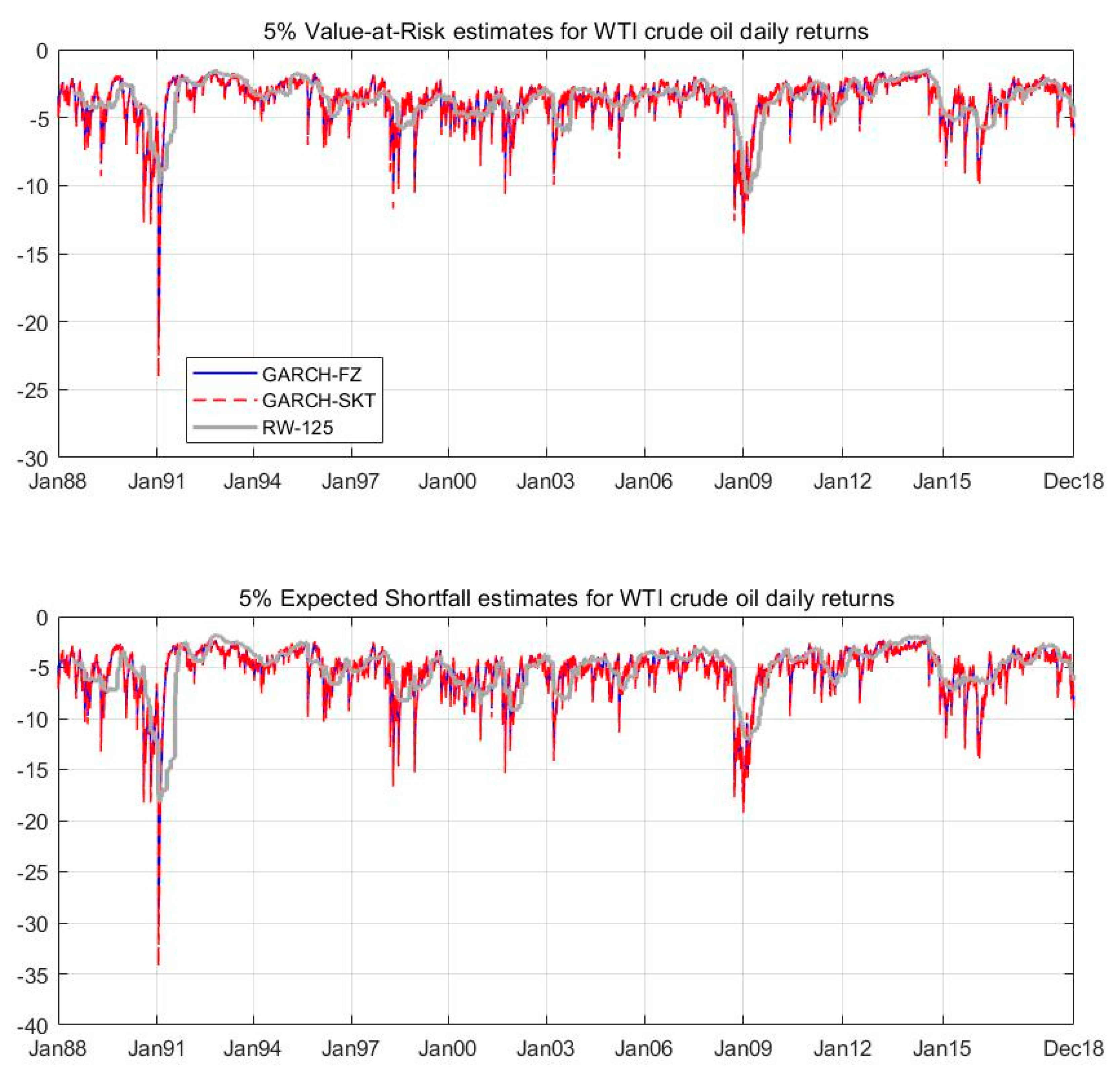
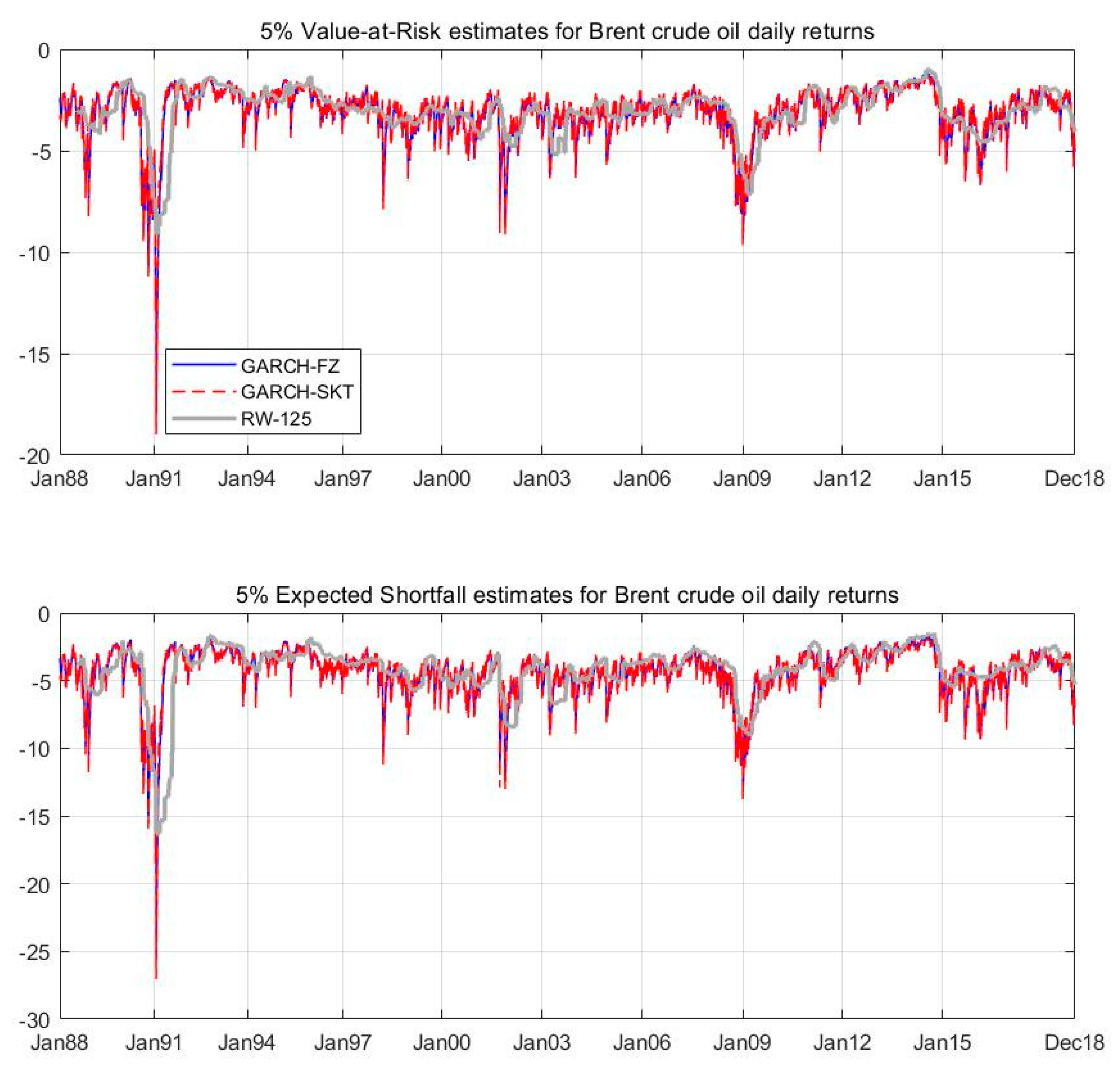
Finally, we provide the fitted 5% ES and VaR values for the three types of models by selecting the best-performing model in the subgroup—that is, the rolling-window model (125 days), the GARCH-SKT model, and the GARCH-FZ model. As Figure 2 and Figure 3 show, the WTI crude oil VaR and ES values were found to be more volatile than those of the Brent crude oil. The most extreme ES values were observed during the Gulf War, with an estimated 35% decrease for the WTI crude oil and a 30% decrease for the Brent crude oil. The second most extreme ES values occurred during the 2008 global financial crisis, with a decrease of approximately 15% for the WTI crude oil and a 10% decrease for the Brent crude oil, which are similar to the findings of Do and Bhatti [37], Wu et al. [38] and Parker and Bhatti [39].

4.2. VaR and ES for the Wavelet

By following the same procedures for the VaR and ES as those of the original crude oil return, we considered the VaR and ES for the wavelet. Specifically, we decomposed the original crude oil return into eight wavelet details (i.e., D1 to D8). We considered the time scales from D1 to D4 as the short-term scale, from D5 to D6 as the mid-term scale, and from D7 to D8 as the long-term scale. (Specifically, D1 denotes a 2 day scale, D2 denotes a 4 day scale, D3 denotes an 8 day scale, D4 denotes a 16 day scale, D5 denotes a 32 day scale, D6 denotes a 64 day scale, D7 denotes a 128 day scale, and D8 denotes a 256 day scale.)

For simplicity, we report the average loss of the model forecasts based on the FZ0 loss function for these wavelet details in

Table 6. The out-of-sample average losses for the wavelet details ($\alpha$ = 0.05).

	D1	D2	D3	D4	D5	D6	D7	D8
Panel A: WTI crude oil
GARCH-N	1.123	0.695	0.168	−0.312	−0.877	−1.338	−1.774	−2.195
GARCH-SKT	1.121	0.695	0.165	−0.326	−0.782	−1.199	−1.621	−2.008
GARCH-EDF	1.121	0.694	0.163	−0.327	−0.939	−1.509	−2.031	−2.566
GAS-1F	1.234	0.834	0.346	−0.333	−1.217	−1.664	−2.950	−3.802
GARCH-FZ	1.115	0.690	0.165	−0.353	−0.939	−1.519	−2.108	−2.566
Hybrid	1.191	0.792	0.235	−0.390	−1.207	−1.318	−2.910	−3.943
Panel B: Brent crude oil
GARCH-N	0.943	0.528	0.019	−0.482	−1.058	−1.482	−1.847	−2.327
GARCH-SKT	0.943	0.529	0.020	−0.465	−0.963	−1.347	−1.693	−2.128
GARCH-EDF	0.942	0.529	0.018	−0.475	−1.119	−1.647	−2.103	−2.321
GAS-1F	1.064	0.682	0.217	−0.498	−1.046	−2.239	−3.011	−4.134
GARCH-FZ	0.940	0.525	0.014	−0.509	−1.205	−1.647	−2.193	−4.111
Hybrid	1.051	0.603	0.208	−0.498	−1.347	−2.237	−3.036	−4.201

Note: The left panel of this table presents the average losses using the FZ0 loss function for the WTI and Brent crude oil return series over the out-of-sample period from January 2000 to December 2018 for 10 different forecasting models. The lowest average loss in each column is highlighted in bold; the second lowest is highlighted in italics. The first three rows correspond to the GARCH forecasts based on different models for the standardized residuals, and the last three rows correspond to the VaR and ES GAS model forecasts.

. Panel A summarizes the average loss for the WTI crude oil, and Panel B summarizes the average loss for the Brent crude oil. The lowest values in each column are denoted in bold. Panel A shows that the GARCH-FZ model is the best choice for D1 and D2; the GARCH-EDF model is the best choice for D3; the GAS-1F model is the best choice for D5, D6, and D7; the hybrid model is the best choice for D4 and D8. Panel B shows that the GARCH-FZ model is the best choice for D1 to D4; the hybrid model is the best choice for D5, D7, and D8; the GAS-1F model is the best choice for D6. Overall, regardless of whether we examined the WTI or the Brent crude oil, the semiparametric models significantly outperformed the nonparametric models.

Similarly, the DM t-statistics for the VaR and ES of the WTI and Brent crude oils are presented in

Table 7. The Diebold−Mariano t-statistics for the average out-of-sample loss differences ($\alpha$ = 0.05, WTI).

	GCH-N	GCH-SKT	GCH-EDF	GAS-1F	GCH-FZ	Hybrid
Panel A: D1 component
GCH-N		2.543	2.459	−4.785	2.439	−3.262
GCH-SKT	−2.543		0.580	−4.902	2.085	−3.379
GCH-EDF	−2.459	−0.580		−4.888	1.948	−3.372
GAS-1F	4.785	4.902	4.888		5.361	4.994
GCH-FZ	−2.439	−2.085	−1.948	−5.361		−3.893
Hybrid	3.262	3.379	3.372	−4.994	3.893
Panel B: D2 component
GCH-N		0.384	0.920	−7.193	2.925	−6.793
GCH-SKT	−0.384		0.889	−7.219	2.998	−6.813
GCH-EDF	−0.920	−0.889		−7.219	2.740	−6.833
GAS-1F	7.193	7.219	7.219		7.767	2.888
GCH-FZ	−2.925	−2.998	−2.740	−7.767		−7.321
Hybrid	6.793	6.813	6.833	−2.888	7.321
Panel C: D3 component
GCH-N		2.530	2.228	−8.528	−6.846	0.814
GCHSKT	−2.530		1.902	−8.642	−6.980	0.124
GCH-EDF	−2.228	−1.902		−8.698	−7.076	−0.508
GAS-1F	8.528	8.642	8.698		0.813	8.538
GCH-FZ	6.846	6.980	7.076	−0.813		6.765
Hybrid	−0.814	−0.124	0.508	−8.538	−6.765
Panel D: D4 component
GCH-N		3.813	2.846	1.150	4.933	4.272
GCH-SKT	−3.813		0.586	0.389	3.056	3.520
GCH-EDF	−2.846	−0.586		0.334	2.783	3.451
GAS-1F	−1.150	−0.389	−0.334		1.078	3.581
GCH-FZ	−4.933	−3.056	−2.783	−1.078		2.356
Hybrid	−4.272	−3.520	−3.451	−3.581	−2.356
Panel E: D5 component
GCH-N		−19.412	3.791	7.023	3.785	7.023
GCH-SKT	19.412		7.581	8.830	7.573	8.829
GCH-EDF	−3.791	−7.581		5.969	−0.114	5.969
GAS-1F	−7.023	−8.830	−5.969		−5.970	−1.933
GCH-FZ	−3.785	−7.573	0.114	5.970		5.970
Hybrid	−7.023	−8.829	−5.969	1.933	−5.970
Panel F: D6 component
GCH-N		−36.715	8.174	5.425	8.168	−0.266
GCH-SKT	36.715		12.564	7.676	12.555	1.591
GCH-EDF	−8.174	−12.564		2.387	1.308	−2.702
GAS-1F	−5.425	−7.676	−2.387		−2.386	−5.713
GCH-FZ	−8.168	−12.555	−1.308	2.386		−2.702
Hybrid	0.266	−1.591	2.702	5.713	2.702
Panel G: D7 component
GCH-N	NaN	−52.041	8.312	10.176	18.997	7.745
GCH-SKT	52.041		12.292	11.440	25.120	8.744
GCH-EDF	−8.312	−12.292		8.279	3.767	6.396
GAS-1F	−10.176	−11.440	−8.279		−7.617	−0.665
GCH-FZ	−18.997	−25.120	−3.767	7.617		5.728
Hybrid	−7.745	−8.744	−6.396	0.665	−5.728
Panel H: D8 component
GCH-N		−60.458	11.633	9.118	11.629	9.612
GCH-SKT	60.458		16.388	10.119	16.384	10.589
GCH-EDF	−11.633	−16.388		7.511	−0.431	8.014
GAS-1F	−9.118	−10.119	−7.511		−7.512	3.575
GCH-FZ	−11.629	−16.384	0.431	7.512		8.014
Hybrid	−9.612	−10.589	−8.014	−3.575	−8.014

Note: This table presents the t-statistics of the Diebold−Mariano tests that were used to compare the average losses using the FZ0 loss function over the out-of-sample period from January 2000 to December 2018 for 10 different forecasting models. A positive value indicates that the row model has a higher average loss than that of the column model. Absolute values greater than 1.96 indicate that the average loss is significantly different from zero at the 95% confidence level. Values along the main diagonal are all zero and were omitted for interpretability. The first three GARCH forecasts are based on different models for the standardized residuals, and the last three rows correspond to the VaR and ES GAS model forecasts.

and

Table 8. The Diebold−Mariano t-statistics for the average out-of-sample loss differences ($\alpha$ = 0.05, Brent oil).

	GCH-N	GCH-SKT	GCH-EDF	GAS-1F	GCH-FZ	Hybrid
Panel A: D1 component
GCH-N		−0.151	1.274	−6.382	1.902	−5.770
GCH-SKT	0.151		1.098	−6.396	2.107	−5.773
GCH-EDF	−1.274	−1.098		−6.456	1.661	−5.822
GAS-1F	6.382	6.396	6.456		6.543	0.596
GCH-FZ	−1.902	−2.107	−1.661	−6.543		−5.906
Hybrid	5.770	5.773	5.822	−0.596	5.906
Panel B: D2 component
GCH-N		−0.178	−0.772	−7.923	1.892	−6.403
GCH-SKT	0.178		−0.448	−7.959	2.071	−6.438
GCH-EDF	0.772	0.448		−7.934	2.064	−6.411
GAS-1F	7.923	7.959	7.934		8.233	4.600
GCH-FZ	−1.892	−2.071	−2.064	−8.233		−6.829
Hybrid	6.403	6.438	6.411	−4.600	6.829
Panel C: D3 component
GCH-N		−2.060	1.476	−7.067	4.623	−5.977
GCH-SKT	2.060		2.901	−7.014	4.754	−5.963
GCH-EDF	−1.476	−2.901		−7.077	4.026	−6.000
GAS-1F	7.067	7.014	7.077		7.251	0.440
GCH-FZ	−4.623	−4.754	−4.026	−7.251		−6.110
Hybrid	5.977	5.963	6.000	−0.440	6.110
Panel D: D4 component
GCH-N		−4.671	−1.283	0.736	3.489	0.736
GCH-SKT	4.671		1.135	1.373	4.967	1.373
GCH-EDF	1.283	−1.135		1.067	3.949	1.067
GAS-1F	−0.736	−1.373	−1.067		0.455	1.006
GCH-FZ	−3.489	−4.967	−3.949	−0.455		−0.455
Hybrid	−0.736	−1.373	−1.067	−1.006	0.455
Panel E: D5 component
GCH-N		−18.293	3.627	−0.197	12.452	8.205
GCH-SKT	18.293		7.209	1.346	15.474	10.579
GCH-EDF	−3.627	−7.209		−1.282	7.641	6.872
GAS-1F	0.197	−1.346	1.282		2.870	7.872
GCH-FZ	−12.452	−15.474	−7.641	−2.870		4.529
Hybrid	−8.205	−10.579	−6.872	−7.872	−4.529
Panel F: D6 component
GCH-N		−32.611	6.957	7.524	6.952	7.521
GCH-SKT	32.611		11.018	8.763	11.011	8.760
GCH-EDF	−6.957	−11.018		6.374	0.035	6.372
GAS-1F	−7.524	−8.763	−6.374		−6.375	0.556
GCH-FZ	−6.952	−11.011	−0.035	6.375		6.373
Hybrid	−7.521	−8.760	−6.372	−0.556	−6.373
Panel G: D7 component
GCH-N		−41.314	8.187	8.893	22.234	6.780
GCH-SKT	41.314		11.901	10.007	28.020	7.615
GCH-EDF	−8.187	−11.901		7.187	3.933	5.764
GAS-1F	−8.893	−10.007	−7.187		−6.478	0.240
GCH-FZ	−22.234	−28.020	−3.933	6.478		4.980
Hybrid	−6.780	−7.615	−5.764	−0.240	−4.980
Panel H: D8 component
GCH-N		−74.639	6.972	10.917	11.057	2.327
GCH-SKT	74.639		7.618	12.124	12.239	2.128
GCH-EDF	−6.972	−7.618		−1.785	−1.466	4.450
GAS-1F	−10.917	−12.124	1.785		2.314	4.134
GCH-FZ	−11.057	−12.239	1.466	−2.314		4.201
Hybrid	−2.327	−2.128	−4.450	−4.134	−4.201

Note: This table presents the t-statistics for the Diebold–Mariano tests that were used to compare the average losses using the FZ0 loss function over the out-of-sample period from January 2000 to December 2018 for 10 different forecasting models. A positive value indicates that the row model has a higher average loss than that of the column model. Absolute values greater than 1.96 indicate that the average loss is significantly different from zero at the 95% confidence level. Values along the main diagonal are all zero and were omitted for interpretability. The first three GARCH forecasts are based on different models for the standardized residuals, and the last three rows correspond to the VaR and ES GAS model forecasts.

. The DM t-statistics were found to be positive for the models with the best fit, as discussed above. For example, the GARCH-FZ model contains all positive entries for D1 and D2, implying that it outperformed all the competing models. This is significant when comparing the three parametric GARCH-N models. The GARCH-EDF model contains all positive entries for D3, with the only exception being the hybrid model, with a DM t-statistic of 0.508. We obtained the same results for the DM t-statistics of the Brent crude oil VaR and ES. Overall, we confirmed that the semiparametric model performs better than the nonparametric models.

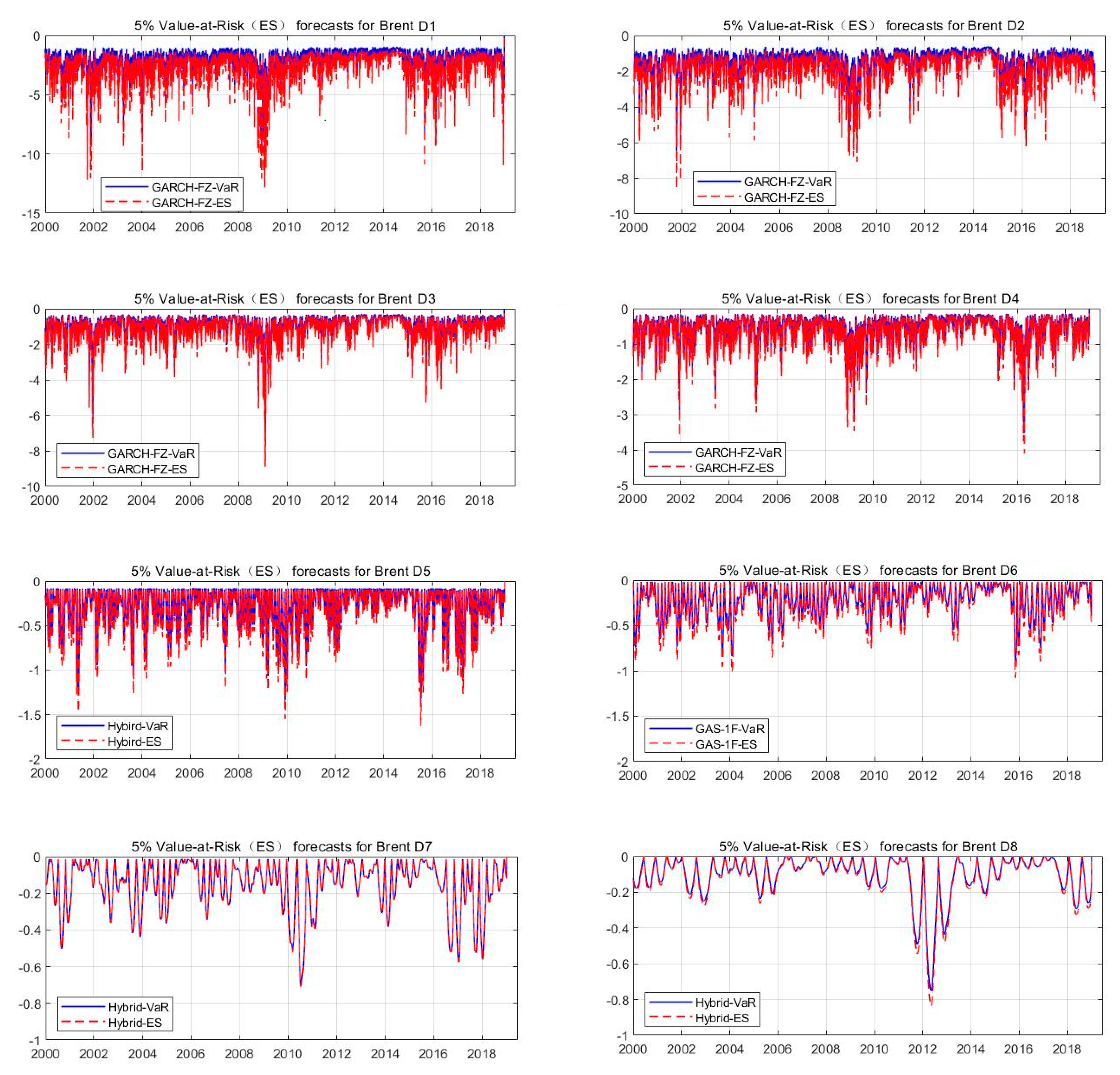
Furthermore, the fitted 5% ES and VaR for the best-performing model for each time scale according to the lowest average loss are summarized in Table 6. Figure 4 plots the forecasts of ES and VaR for the WTI crude oil, and Figure 5 plots the forecasts for the Brent crude oil. The wavelet details for the WTI crude oil VaR and ES were found to be more volatile than those for the Brent crude oil. Moreover, the volatility of the VaR and ES decreased as the time scale increased. The results are similar to those of Fernandez [7]—that is, the variance in the VaR and ES stems mainly from the short-term wavelet components. Moreover, the GARCH-FZ model was found to be driven only by information when the VaR was violated, which indicates a deterministic reversion to the long-run mean on the following day. Thus, the behaviors of the VaR and ES for the GARCH-FZ model are smoother than those of the other models.

4.3. Further Robustness Tests

To ensure the robustness of our results, we considered the average loss across four different tails: $\alpha$ values of 0.10, 0.05, 0.025, and 0.01. We used this procedure to investigate the performance of the models in their response to changes based on the depths of the tails (see

Table 9. The out-of-sample performance rankings for various alpha values.

		WTI					Brent Oil
	$\mathit{\alpha }$ = 0.01	$\mathit{\alpha }$ = 0.025	α = 0.05	$\mathit{\alpha }$ = 0.10	Ave	$\mathit{\alpha }$ = 0.01	$\mathit{\alpha }$ = 0.025	$\mathit{\alpha }$ = 0.05	$\mathit{\alpha }$ = 0.10	Ave
Panel A: Raw data
RW-125	5	6	6	6	5.75	6	7	7	7	6.75
RW-250	8	8	8	8	8	7	8	8	8	7.75
RW-500	9	9	9	9	9	8	9	9	9	8.75
GCH-N	6	5	5	5	5.25	5	5	5	5	5
GCH-SKT	2	2	2	2	2	3	4	3	3	3.25
GCH-EDF	3	4	3	3	3.25	4	3	4	4	3.75
GAS-1F	4	3	4	4	3.75	2	2	2	1	1.75
GCH-FZ	1	1	1	1	1	1	1	1	2	1.25
Hybrid	7	8	7	7	7.25	9	9	6	6	7.5
Panel B: D1 component
GCH-N	4	5	5	5	4.75	4	4	4	4	4
GCH-SKT	3	4	4	4	3.75	3	3	3	3	3
GCH-EDF	1	2	3	3	2.25	1	2	2	2	1.75
GAS-1F	6	6	6	6	6	6	6	6	6	6
GCH-FZ	2	1	1	1	1.25	2	1	1	1	1.25
Hybrid	2	3	2	2	2.25	5	5	5	5	5
Panel C: D2 component
GCH-N	4	2	4	4	3.5	2	2	4	2	2.5
GCH-SKT	3	3	3	3	3	3	3	3	3	3
GCH-EDF	1	4	2	2	2.25	4	4	2	4	3.5
GAS-1F	6	6	6	6	6	6	6	6	6	6
GCH-FZ	2	1	1	1	1.25	1	1	1	1	1
Hybrid	5	5	5	5	5	5	5	5	5	5
Panel D: D3 component
GCH-N	4	4	4	5	4.25	4	4	3	4	3.75
GCH-SKT	3	2	2	4	2.75	2	3	4	5	3.5
GCH-EDF	1	1	1	3	1.5	3	2	2	3	2.5
GAS-1F	6	6	6	2	5	6	6	6	6	6
GCH-FZ	2	3	3	6	3.5	1	1	1	2	1.25
Hybrid	5	5	5	1	4	5	5	5	1	4
Panel E: D4 component
GCH-N	3	4	4	5	4	2	2	4	4	3
GCH-SKT	6	6	6	6	6	5	4	6	6	5.25
GCH-EDF	5	5	3	4	4.25	3	3	5	5	4
GAS-1F	4	2	1	2	2.25	6	6	3	2	4.25
GCH-FZ	2	3	2	3	2.5	1	1	1	3	1.5
Hybrid	1	1	5	1	2	4	5	2	1	3
Panel F: D5 component
GCH-N	4	5	6	6	5.25	4	5	3	5	4.25
GCH-SKT	3	4	5	5	4.25	6	4	6	6	5.5
GCH-EDF	2	3	4	4	3.25	3	3	4	4	3.5
GAS-1F	6	6	3	2	4.25	5	6	5	2	4.5
GCH-FZ	1	1	2	3	1.75	1	1	2	3	1.75
Hybrid	5	2	1	1	2.25	2	2	1	1	1.5
Panel G: D6 component
GCH-N	3	4	4	5	4	5	5	5	5	5
GCH-SKT	6	6	6	6	6	6	6	6	6	6
GCH-EDF	5	5	3	4	4.25	3	3	4	4	3.5
GAS-1F	4	2	1	2	2.25	4	4	2	1	2.75
GCH-FZ	2	3	2	3	2.5	5	5	3	2	3.75
Hybrid	1	1	5	1	2	1	1	1	3	1.5
Panel H: D7 component
GCH-N	4	5	5	5	4.75	5	5	5	5	5
GCH-SKT	5	6	6	6	5.75	6	6	3	6	5.25
GCH-EDF	3	4	4	4	3.75	3	4	4	4	3.75
GAS-1F	6	2	1	1	2.5	4	2	2	1	2.25
GCH-FZ	2	3	3	3	2.75	2	3	1	3	2.25
Hybrid	1	1	2	2	1.5	1	1	6	2	2.5
Panel I: D8 component
GCH-N	5	5	5	5	5	5	5	5	5	5
GCH-SKT	6	6	6	6	6	6	6	6	6	6
GCH-EDF	3	4	4	4	3.75	4	4	4	3	3.75
GAS-1F	4	2	2	2	2.5	2	2	2	2	2
GCH-FZ	2	3	3	3	2.75	3	3	3	4	3.25
Hybrid	1	1	1	1	1	1	1	1	1	1

Note: Rankings (with the best performing model ranked 1 and the worst ranked 6) based on the average losses using the FZ0 loss function for the daily crude oil return series over the out-of-sample period from January 2000 to December 2018 for 10 different forecasting models. The last column for each panel shows the average rank across the alpha values.

). For the original WTI crude oil series, the best-performing model was the GARCH-FZ model, followed by the GARCH-SKT model, across different values of $\alpha$. In other words, the GARCH estimated by the FZ0 loss minimization parametrically outperformed the GARCH estimated by the nonparametric residuals. However, for the Brent crude oil, the best-performing model was the GARCH-FZ, followed by GAS-1F, when $\alpha$ was equal to 0.05, 0.025, and 0.01. For $\alpha$ = 0.10, the GAS-FZ model outperformed the GARCH-FZ model, which occurred because the GAS model depends on the observed VaR violation.

When the values of $\alpha$ were very small, these violations rarely occurred. In contrast, the squared residual from the GARCH model provided information flows to move the risk measures, regardless of the VaR violation. If the values of $\alpha$ were not too small, then the GAS model with the FZ0 loss function began to perform well. This is likely because the Brent crude oil price data are less volatile than that of the WTI crude oil price data. Overall, we took the average of the rank in the final column. Clearly, the distribution-based GARCH model is always the second or lower choice.

Since the out-of-sample period was from January 2000 to December 2018, it included the 2008 global financial crisis, which presented a significant structural change in VaR and ES forecasting. To address this structural break, we further determined the results of the performance of the models in terms of their responses to changes, based on the depth of the tails before and after the 2008 global financial crisis (see

Table 10. The out-of-sample performance rankings for various alpha values based on the WTI price.

	1 January 1999 to 31 December 2008					1 January 2009 to 31 December 2018
	$\mathit{\alpha }$ = 0.01	$\mathit{\alpha }$ = 0.025	$\mathit{\alpha }$ = 0.05	$\mathit{\alpha }$ = 0.10	Ave	$\mathit{\alpha }$ = 0.01	$\mathit{\alpha }$ = 0.025	$\mathit{\alpha }$ = 0.05	$\mathit{\alpha }$ = 0.10	Ave
Panel A: Raw data
RW-125	5	6	6	6	5.75	6	7	7	7	6.75
RW-250	8	8	8	8	8	7	8	8	8	7.75
RW-500	9	9	9	9	9	9	9	9	9	9
GCH-N	6	5	5	5	5.25	5	5	5	5	5
GCH-SKT	2	2	2	2	2	3	4	2	2	2.75
GCH-EDF	3	3	3	3	3	4	3	4	4	3.75
GAS-1F	4	4	4	4	4	2	2	3	3	2.5
GCH-FZ	1	1	1	1	1	1	1	1	1	1
Hybrid	7	7	7	7	7	8	8	6	6	7
Panel B: D1 component
GCH-N	4	5	5	5	4.75	4	4	4	4	4
GCH-SKT	3	4	4	4	3.75	3	3	3	3	3
GCH-EDF	1	1	2	3	1.75	2	2	2	2	2
GAS-1F	6	6	6	6	6	6	6	6	6	6
GCH-FZ	2	2	1	1	1.5	1	1	1	1	1
Hybrid	2	3	3	2	2.5	5	5	5	5	5
Panel C: D2 component
GCH-N	4	2	4	4	3.5	2	2	4	2	2.5
GCH-SKT	3	3	3	3	3	3	3	3	3	3
GCH-EDF	2	4	2	2	2.5	4	4	2	4	3.5
GAS-1F	6	6	6	6	6	6	6	6	6	6
GCH-FZ	1	1	1	1	1	1	1	1	1	1
Hybrid	5	5	5	5	5	5	5	5	5	5
Panel D: D3 component
GCH-N	4	4	4	5	4.25	4	4	3	4	3.75
GCH-SKT	3	2	2	4	2.75	2	3	4	5	3.5
GCH-EDF	1	1	1	3	1.5	3	2	2	3	2.5
GAS-1F	6	6	6	2	5	6	6	6	6	6
GCH-FZ	2	3	3	6	3.5	1	1	1	2	1.25
Hybrid	5	5	5	1	4	5	5	5	1	4
Panel E: D4 component
GCH-N	3	4	4	5	4	2	2	4	4	3
GCH-SKT	6	6	6	6	6	5	4	6	6	5.25
GCH-EDF	5	5	3	4	4.25	3	3	5	5	4
GAS-1F	4	2	1	2	2.25	6	6	3	2	4.25
GCH-FZ	2	3	2	3	2.5	1	1	1	3	1.5
Hybrid	1	1	5	1	2	4	5	2	1	3
Panel F: D5 component
GCH-N	4	5	6	6	5.25	4	5	3	5	4.25
GCH-SKT	3	4	5	5	4.25	6	4	6	6	5.5
GCH-EDF	2	3	4	4	3.25	3	3	4	4	3.5
GAS-1F	6	6	3	2	4.25	5	6	5	2	4.5
GCH-FZ	1	1	2	3	1.75	1	1	2	3	1.75
Hybrid	5	2	1	1	2.25	2	2	1	1	1.5
Panel G: D6 component
GCH-N	3	4	4	5	4	5	5	5	5	5
GCH-SKT	6	6	6	6	6	6	6	6	6	6
GCH-EDF	5	5	3	4	4.25	3	3	4	4	3.5
GAS-1F	4	2	1	2	2.25	4	4	2	1	2.75
GCH-FZ	2	3	2	3	2.5	5	5	3	2	3.75
Hybrid	1	1	5	1	2	1	1	1	3	1.5
Panel H: D7 component
GCH-N	4	5	5	5	4.75	5	5	5	5	5
GCH-SKT	5	6	6	6	5.75	6	6	3	6	5.25
GCH-EDF	3	4	4	4	3.75	3	4	4	4	3.75
GAS-1F	6	2	1	1	2.5	4	2	2	1	2.25
GCH-FZ	2	3	3	3	2.75	2	3	1	3	2.25
Hybrid	1	1	2	2	1.5	1	1	6	2	2.5
Panel I: D8 component
GCH-N	5	5	5	5	5	5	5	5	5	5
GCH-SKT	6	6	6	6	6	6	6	6	6	6
GCH-EDF	3	4	4	4	3.75	4	4	4	3	3.75
GAS-1F	4	2	2	2	2.5	2	2	2	2	2
GCH-FZ	2	3	3	3	2.75	3	3	3	4	3.25
Hybrid	1	1	1	1	1	1	1	1	1	1

). For simplicity, we only looked at the forecast results based on the WTI price. As shown in Table 10, although there were slight changes in rankings for the performance of the individual models, the average rankings remained the same. In this sense, our model provided a consistent forecast.

To further explore the performance differences as the time scale changed, we also determined the performance rankings for both the nonparametric models and the semiparametric models. Once again, the semiparametric models always outperformed the nonparametric models. The distribution-based GARCH model was always the second or lower choice for the short-term scales. Specifically, the GARCH-FZ model performed the best for the short-term scales, whereas the hybrid model performed the best for the long-term scales.

Moreover, as the time scale increased, the semiparametric model estimated using FZ0 loss minimization parametrically outperformed the GARCH model estimated using nonparametric residuals, regardless of the type of model. Since the short-term wavelet components are more volatile than the long-term wavelet components, the hybrid model began to perform well for the mid- and long-term scales. In addition, we also identified a similar forecast performance by considering two market regimes across the time scales, as shown in Table 10. Only the short-term scale exhibited variations in the rankings of performance for the individual model without changing the average rankings. For example, for the D6 component of the WTI crude oil, the hybrid model was ranked first, followed by the GAS-1F and GARCH-FZ models. Moreover, as the time scale increased, violations of rank across the values of $\alpha$ rarely occurred for these models, especially for the semiparametric models. At the same time, the wavelet components for the Brent crude oil exhibited similar patterns to those for the WTI crude oil. The results also indicate that the semiparametric models are the best choice when estimating the VaR and ES, regardless of the time scale.

5. Conclusions

Understanding the risk of the crude oil market across time scales is essential for risk management and asset pricing. Conventional analyses of market risk rely on the assumption of the conditional distribution of returns. However, the accuracy of this approach relies on making correct choices for distribution and assumptions. To overcome the problem of distribution-dependent forecasts of the VaR and ES, we developed a wavelet-based approach based on the semiparametric methodology that is independent of assumptions on the distribution. Moreover, we investigated the statistical decision theory to jointly model the dynamic ES and VaR values in order to address the problem of elicitability for ES. We proposed three types of dynamic VaR and ES based on parametric structures and compared their performance with that of the nonparametric forecast models. Our study relaxed the strict assumption about the nonparametric distribution-based model with a more robust result that will help financial practitioners, energy policymakers, and energy economists to improve their forecasting ability for VaR and ES in the crude oil market.

In the empirical analysis, we employed a full sample of the daily WTI and Brent crude oil prices from January 1988 to December 2018 to investigate whether the semiparametric models outperform the nonparametric models in terms of forecasting the VaR and ES in the crude oil market for different time horizons. We used the first 12 years (before 2000) to estimate the parameters and the last 19 years (after 2000) to forecast the VaR and ES under different confidence levels of $\alpha$ for different time scales. The empirical results show that the VaR and ES forecasts based on the GARCH-FZ model outperform those based on the other models for the original crude oil return series. For the wavelet-based VaR and ES forecasts, we found that the GARCH-FZ model performs best in the short term, whereas the hybrid model performs best in the mid and long term. Moreover, as the time scale increases, the semi-parameter models outperform the nonparametric distribution-based model with a decreasing market risk in the crude oil market. Overall, we found that our proposed semiparametric model outperforms the nonparametric model, regardless of the time scale.

Our findings have several implications. Firstly, investors should choose their distributions or investment horizons carefully when building their risk forecast models. A semiparametric model provides more robust results in the crude oil market than a parametric model, regardless of the time scale. It also improves the accuracy of risk and portfolio management for different time horizons. Secondly, by introducing a wavelet analysis into the semiparametric VaR and ES measures, our proposed models allow risk managers to evaluate the extreme crude oil risk under different investment horizons in highly volatile environments, by considering the GARCH-FZ model in the short term and by considering the hybrid model in the long term. The ES measure is especially effective for measuring extreme risk for the crude oil market. Thirdly, with fewer assumptions of the conditional distribution in the VaR and ES model, policymakers can create appropriate crude oil policies, because they can easily model the influence of crude oil risk on the real economy. Specifically, by using the appropriate energy policy to stabilize the oil price fluctuations, the negative outcome to the economy from oil shock will be alleviated.

References

1. Hammoudeh, S.; Santos, P.A.; Al-Hassen, A. Downside risk management and VaR based optimal portfolios for precious metals, oil and stocks. N. Am. J. Econ. Financ. 2013, 25, 318–334. [Google Scholar] [CrossRef]
2. Pérignon, C.; Smith, D. The level and quality of value-at-risk disclosure by commercial banks. J. Bank Financ. 2010, 34, 362–377. [Google Scholar] [CrossRef]
3. Aloui, C.; Mabrouk, S. Value-at-risk estimations of energy commodities via long memory, asymmetry and fat-tailed GARCH models. Energ. Policy 2010, 38, 2326–2339. [Google Scholar] [CrossRef]
4. Costello, A.; Asem, E.; Gardner, E. Comparison of historically simulated VaR: Evidence from oil prices. Energ. Econ. 2008, 30, 2154–2166. [Google Scholar] [CrossRef]
5. Cifter, A. Value-at-risk estimation with wavelet-based extreme value theory: Evidence from emerging markets. Physica A 2011, 390, 2356–2367. [Google Scholar] [CrossRef]
6. Fan, Y.; Zhang, Y.J.; Tsai, H.T.; Wei, Y.M. Estimating “value-at-risk” of crude oil price and its spillover effect using the GED-GARCH approach. Energ. Econ. 2008, 30, 3156–3171. [Google Scholar] [CrossRef]
7. Fernandez, V. The CAPM and value at risk at different time-scales. Int. Rev. Financ. Anal. 2006, 15, 203–219. [Google Scholar] [CrossRef]
8. Tolikas, K. Unexpected tails in risk measurement: Some international evidence. J. Bank Financ. 2014, 40, 476–493. [Google Scholar] [CrossRef]
9. Youssef, M.; Belkacem, L.; Mokni, K. Value-at-risk estimation of energy commodities: A long-memory GARCH-EVT approach. Energ. Econ. 2015, 51, 99–110. [Google Scholar] [CrossRef]
10. Lyu, Y.; Wang, P.; Wei, Y.; Ke, R. Forecasting the VaR of crude oil market: Do alternative distributions help? Energ. Econ. 2017, 66, 523–534. [Google Scholar] [CrossRef]
11. Zhao, L.T.; Liu, K.; Duan, X.L.; Li, M.F. Oil price risk evaluation using a novel hybrid model based on time-varying long memory. Energ. Econ. 2019, 81, 70–78. [Google Scholar] [CrossRef]
12. Artzner, P.; Delbaen, F.; Eber, J.M.; Heath, D. Coherent measures of risk. Math. Financ. 1999, 9, 203–228. [Google Scholar] [CrossRef]
13. Fissler, T.; Ziegel, J.F. Higher-order elicitability and Osband’s principle. Ann. Stat. 2016, 44, 1680–1707. [Google Scholar] [CrossRef]
14. Boubaker, H.; Sghaier, N. Semiparametric generalized long-memory modeling of some MENA stock market returns: A wavelet approach. Econ. Model. 2015, 50, 254–265. [Google Scholar] [CrossRef]
15. Zhou, X.; Lin, J. Asymptotic properties of wavelet estimators in semiparametric regression models under dependent errors. J. Multivar. Anal. 2013, 122, 251–270. [Google Scholar] [CrossRef]
16. Creal, D.D.; Koopman, S.J.; Lucas, A. Generalized autoregressive score models with applications. J. Appl. Econ. 2013, 28, 777–795. [Google Scholar] [CrossRef] [Green Version]
17. He, K.; Xie, C.; Chen, S.; Lai, K.K. Estimating VaR in crude oil market: A novel multi-scale non-linear ensemble approach incorporating wavelet analysis and neural network. Neurocomputing 2009, 72, 3428–3438. [Google Scholar] [CrossRef]
18. Engle, R.F.; Manganelli, S. CAViaR: Conditional autoregressive value at risk by regression quantiles. J. Bus. Econ. Stat. 2004, 22, 367–381. [Google Scholar] [CrossRef]
19. Nolde, N.; Ziegel, J.F. Elicitability and backtesting: Perspectives for banking regulation. Ann. Appl Stat. 2017, 11, 1833–1874. [Google Scholar] [CrossRef]
20. Engle, R.F.; Manganelli, S. A comparison of value-at-risk models in finance. In Risk Measures for the 21st Century; Szego, G., Ed.; Wiley: Hoboken, NJ, USA; Chichester, UK, 2004. [Google Scholar]
21. Peng, W.; Hu, S.; Chen, W.; Zeng, Y.; Yang, L. Modeling the joint dynamic value at risk of the volatility index, oil price, and exchange rate. Int. Rev. Econ. Financ. 2019, 59, 137–149. [Google Scholar] [CrossRef]
22. Wen, D.; Wang, G.J.; Ma, C.; Wang, Y. Risk spillovers between oil and stock markets: A VAR for VaR analysis. Energ Econ. 2019, 80, 524–535. [Google Scholar] [CrossRef]
23. Diebold, F.X.; Mariano, R.S. Comparing predictive accuracy. J. Bus. Econ. Stat. 1995, 13, 253–263. [Google Scholar]
24. Taylor, J.W. Forecasting value at risk and expected shortfall using a semiparametric approach based on the asymmetric Laplace distribution. J. Bus. Econ. Stat. 2017, 37, 121–133. [Google Scholar] [CrossRef]
25. Percival, D.B.; Walden, A. Wavelet Methods for Time Series Analysis; Cambridge University Press: Cambridge, UK, 2000. [Google Scholar]
26. Yang, L.; Yang, L.; Hoo, G.; Hamori, S. Dependence structures and risk spillover in China’s credit bond market: A copula and CoVaR approach. J. Asian Econ. 2020, 68, 101200. [Google Scholar] [CrossRef]
27. Cabedo, J.D.; Moya, I. Estimating oil price “value at risk” using the historical simulation approach. Energ. Econ. 2003, 25, 239–253. [Google Scholar] [CrossRef]
28. Gençay, R.; Selçuk, F.; Ulugulyagci, A. High volatility, thick tails and extreme value theory in value-at-risk estimation. Insur. Math. Econ. 2003, 33, 337–356. [Google Scholar] [CrossRef] [Green Version]
29. Gençay, R.; Selçuk, F. Extreme value theory and value-at-risk: Relative performance in emerging markets. Int. J. Forecast. 2004, 20, 287–303. [Google Scholar] [CrossRef] [Green Version]
30. Bollerslev, T. Generalized autoregressive conditional heteroskedasticity. J. Econ. 1986, 31, 307–327. [Google Scholar] [CrossRef] [Green Version]
31. Hansen, B.E. Autoregressive conditional density estimation. Int. Econ. Rev. 1994, 35, 705–730. [Google Scholar] [CrossRef]
32. Yuan, N.; Yang, L. Asymmetric risk spillover between financial market uncertainty and the carbon market: A GAS–DCS–copula approach. J. Clean Prod. 2020, 59, 25920. [Google Scholar] [CrossRef]
33. Patton, A.J.; Ziegel, J.F.; Chen, R. Dynamic semiparametric models for expected shortfall (and value-at-risk). J. Econ. 2019, 211, 388–413. [Google Scholar] [CrossRef] [Green Version]
34. Patton, A.J.; Sheppard, K. Optimal combinations of realised volatility estimators. Int. J. Forecast. 2009, 25, 218–238. [Google Scholar] [CrossRef]
35. Christoffersen, P.F. Evaluating interval forecasts. Int. Econ. Rev. 1998, 39, 841–862. [Google Scholar] [CrossRef]
36. Engle, R.F.; Russell, J.R. Autoregressive conditional duration: A new model for irregularly spaced transaction data. Econometrica 1998, 66, 1127–1162. [Google Scholar] [CrossRef]
37. Do, Q.H.; Bhatti, M.I. Is ‘Oil and Gas’ Industry of ASEAN5 countries integrated with the US counterpart? Appl. Econ. 2020, 52, 1–23. [Google Scholar] [CrossRef]
38. Wu, K.; Zhu, J.; Xu, M.; Yang, L. Can crude oil drive the co-movement among the international stock market? N. Am. J. Econ. Financ. 2020, 53, 101194. [Google Scholar] [CrossRef]
39. Parker, S.; Bhatti, M. Dynamics and drivers of per capita CO2 emissions in Asia. Energ. Econ. 2020. [Google Scholar] [CrossRef]
Figure 1. The plots of the raw data for the WTI and Brent crude oil prices.
Energies 13 03700 g001
Figure 2. The estimated 5% VaR and ES values for the daily returns on the WTI crude oil price for the period of January 1988 to December 2018. The estimates were based on a one-factor GAS model, a GARCH model, and a rolling-window model, using 125 observations.
Energies 13 03700 g002
Figure 3. The estimated 5% VaR and ES values for the daily returns on the Brent crude oil price for the period of January 1988 to December 2018. The estimates were based on a one-factor GAS model, a GARCH model, and a rolling-window model, using 125 observations.
Energies 13 03700 g003
Figure 4. The forecasted 5% VaR and ES values for the wavelet of the WTI crude oil price over the period of January 2000 to December 2018. The estimates are based on the model with the best fit from Table 6.
Energies 13 03700 g004
Figure 5. The forecasted 5% VaR and ES for the wavelet of the Brent crude oil price over the period of January 2000 to December 2018. The estimates are based on the model with the best fit from Table 6.
Energies 13 03700 g005