Supertwisting Sliding Mode Algorithm Based Nonlinear MPPT Control for a Solar PV System with Artificial Neural Networks Based Reference Generation

Abstract

The problem of extracting maximum power from a photovoltaic (PV) system with negligible power loss is concerned with the power generating capability of the PV array and nature of the output load. Changing weather conditions and nonlinear behavior of PV systems pose a challenge in tracking of varying maximum power point. A robust nonlinear controller is required to ensure maximum power point tracking (MPPT) by handling nonlinearities of a system and making it robust against changing environmental conditions. Sliding mode controller is robust against disturbances, model uncertainties and parametric variations. It depicts undesirable phenomenon like chattering, inherent in it causing power and heat losses. In this paper, a supertwisting sliding mode algorithm based nonlinear robust controller has been designed for MPPT of a PV system which not only removes the chattering but also enhances the overall system’s dynamic response. Moreover, supertwisting sliding mode controller is robust against changing environmental conditions like change in temperature and irradiance. Noninverting DC-DC Buck-Boost converter has been used as an interface between source and the load. The efficiency of MPPT of a PV system depends upon the accuracy of reference for peak power voltage, therefore an efficient mechanism for reference generation has also been proposed in this work. The reference for peak power voltage has been generated by using a trained artificial neural network, which is to be tracked by proposed nonlinear controllers. Sliding mode controller (SMC) and synergetic controllers have also been designed for MPPT of a PV system in order to compare them with supertwisting sliding mode controller (ST-SMC). Global asymptotic stability of the system has been ensured by using Lyapunov stability criterion. The performance of the proposed nonlinear controllers has been validated in MATLAB/Simulink ODE 45 environment. ST-SMC has also been compared with recently proposed integral backstepping controller and other conventional MPPT controllers given in the literature. The simulation results show the better performance of ST-SMC in terms of best dynamic response and robustness.

1. Introduction

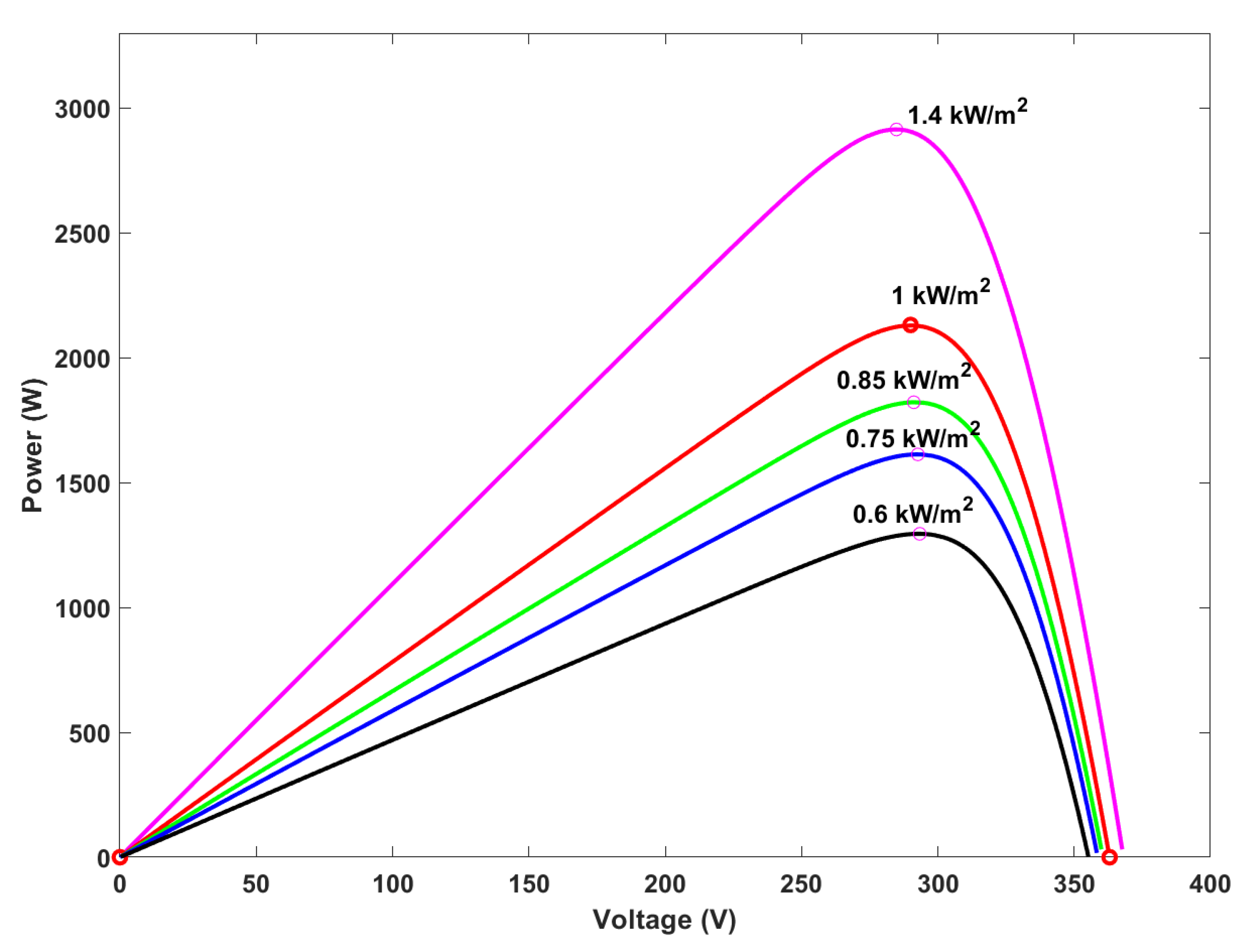
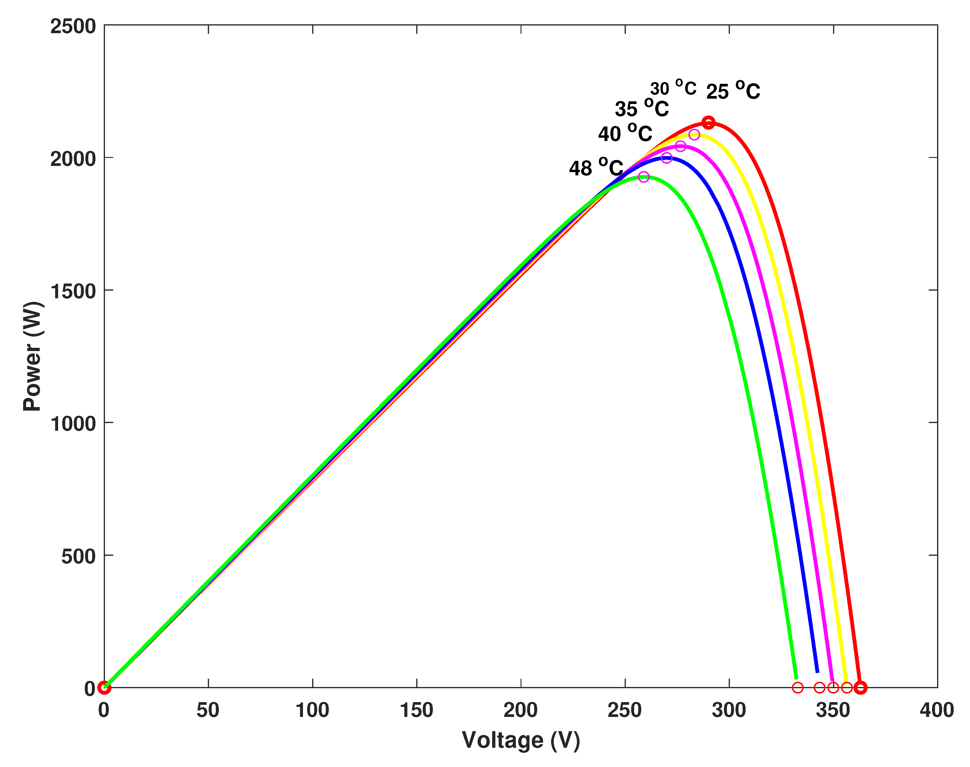
Solar energy is a limitless and clean source of power generation available nowadays. Due to continuous depletion and dangerous environmental effects of conventional energy sources [1], the demand of renewable energy sources especially the solar energy is increasing day by day which can be harvested by the use of solar panels. One major issue with solar panels is their efficiency which is dependent directly on the operating point of the solar cell. 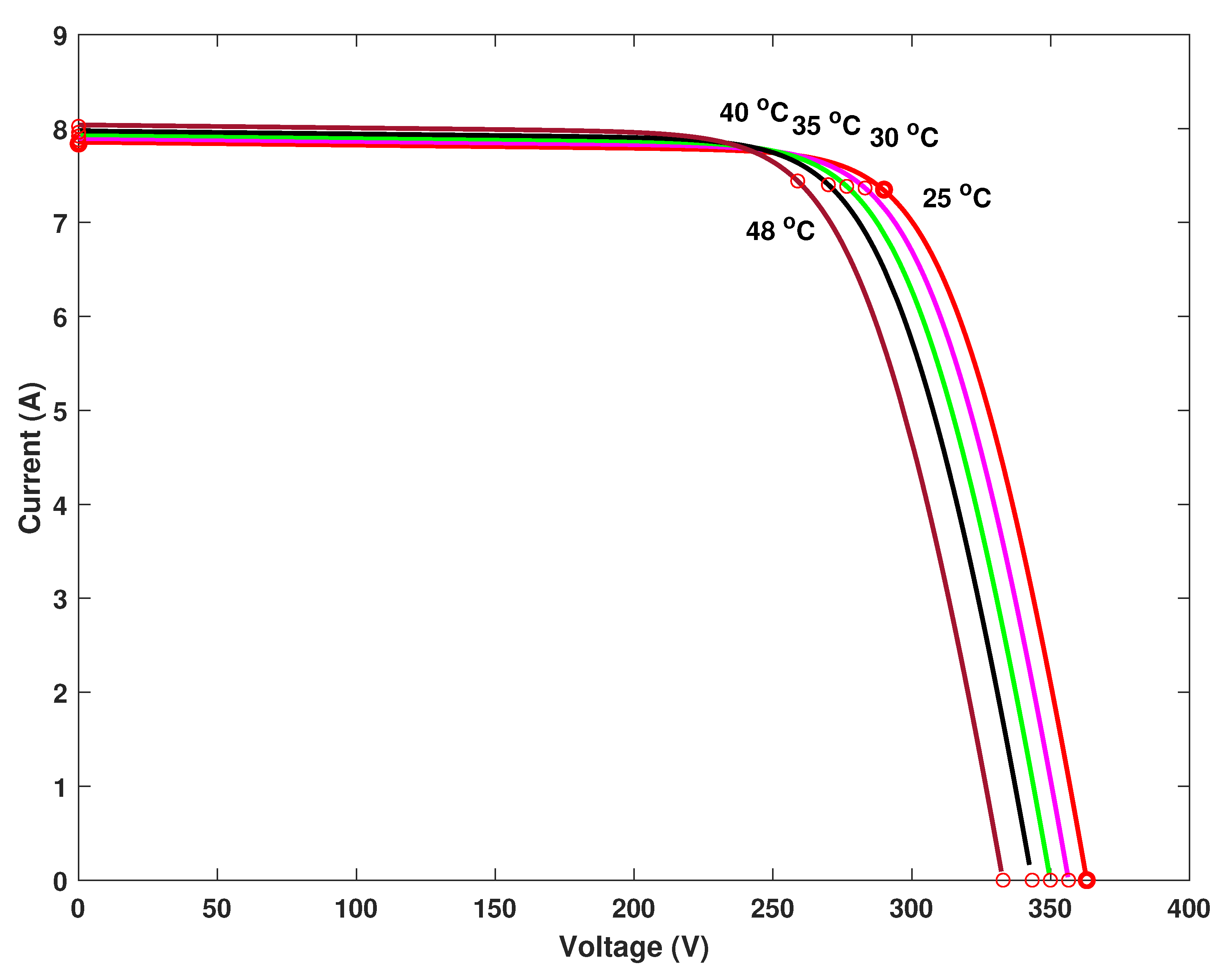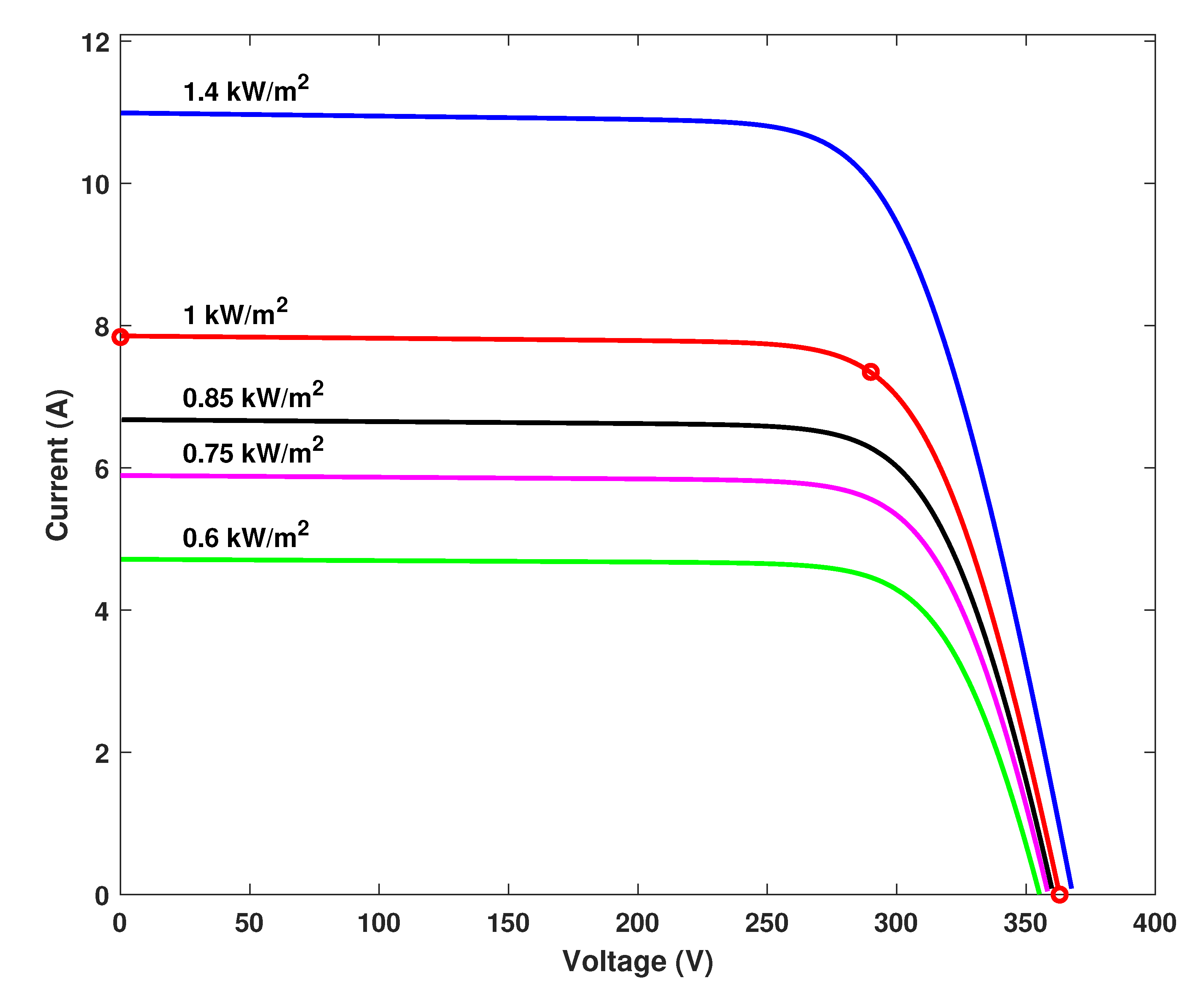The P–V characteristic curves of a photovoltaic (PV) module have been shown in Figure 1 and Figure 2 which show the variation of PV current drawn with varying output voltage. The changing current varies the power extracted from the PV module as shown by the I–V characteristic curves in Figure 3 and Figure 4.

This shows the variation of efficiency and renders the direct connection of load with the PV module. To overcome this problem a DC-DC converter is used as an interface between the PV array and load. The duty cycle of converter is varied in such a manner so as to extract the maximum current required for maximum power extraction by operating the module at maximum power point voltage [2]. Nevertheless, changing environmental factors like irradiance and temperature alter the maximum power point voltage; therefore tracking peak power voltage is crucial task for the maximum power point tracking (MPPT) of a solar PV system.

An extensive research has been done for designing MPPT algorithms using various control techniques. Almost all the algorithms try to drive the PV cell at maxima of either $V_{\mathrm{MPP}}$ or $I_{\mathrm{MPP}}$ which ultimately makes the system to extract maximum power from it. The basic classification of MPPT methods can be divided into following categories:

• Indirect methods,
• Direct methods,
• Soft-computing based methods,
• Linear Controllers,
• Nonlinear Controllers.

Conventionally, an indirect method called constant voltage method is used for MPPT in which open circuit voltage $V_{\mathrm{OC}}$ is sampled either directly by using the voltage of the whole panel or by using the equivalent pilot cell [3]. Reference voltage is thus generated and duty ratio of the converter is then adjusted to make $V_{\mathrm{PV}}=V_{\mathrm{REF}}$. This method is the simplest of all available methods but it requires the disconnection of circuit frequently and is used where only slow or negligible variation in temperature is observed. In constant current method PV is operated at maximum current instead of maximum voltage and has same pros and cons as that of constant voltage method. Some more methods like curve fitting and look up table methods fall in the category of indirect methods.

Direct methods are more suitable than indirect ones because they are faster and do not require the disconnection of PV circuitry. Refs. [4,5] presented the perturb and observe algorithm (P&O) along with its different variants in which the operating point of the panel oscillates around the maximum power point. The basic principle of this method is to observe the change of power by perturbing the operating voltage in regular intervals. If the change $\frac{dP}{dV}$ is positive then the operating point is behind the MPP and if there is a negative change then the operating point is ahead of MPP. $\frac{dP}{dV}=0$ indicates that operating point reaches the maximum power point. Although this method is easy to implement yet it shows oscillations around MPP and is not suitable for fast changing conditions.

Oscillations can be reduced by reducing the step size of perturbation but this also slows down the MPPT. Moreover it requires the measurements of both current and voltage for its operation. Hill climbing method [6] is the variation of P&O algorithm in which perturbation is done in duty ratio instead of perturbing the terminal voltage. Another advanced version of perturb and observe algorithm is the estimated perturb-perturb method (EPP) which is presented in [7], has two modes of operation which are estimation mode and perturbation mode. Estimation mode complements the perturbation mode which calculates the MPP over PV characteristic curve. The compensation by estimation mode is done for irradiance changes only. However temperature changes need to be taken into account.

Incremental conductance (IC) method [8,9] is another direct control method for MPPT. In this method incremental conductance $\frac{dI}{dV}$ is compared to instantaneous conductance $\frac{I}{V}$ and at MPP the sum of both the conductances is equal to zero $(\frac{dI}{dV}+\frac{I}{V}=0)$. It is more efficient than the P&O algorithm [10,11] as it produces less oscillations once the MPP is reached and is robust against rapid weather changes. However, it requires more computations and there are hardware complexities in its implementation as compared to P&O algorithm.

Most of the algorithms for MPPT require system model for their implementation. Fuzzy logic (FLC) controllers are based on human reasoning instead of relying on mathematical model of a system. Membership functions are used [12,13] against each variable which needs to be controlled and assigned values are in the range from 0 to 1. If-else statement based rules are used to map input and output values. Comparison of FLC with IC and P&O shows better performance of FLC [14] due to robustness with the sufficient knowledge of system in hand. Non-availability of exact information about the system is the major disadvantage of FLC based algorithm. Artificial neural network (ANN) based controllers [15,16] require trained data for updating the weights of the neurons. However their efficiency depend upon the extent of training and quality of trained data.

Bio-inspired algorithms due to computational burden are sometimes ineffective in terms of iterations needed for continuously tracking the MPP. This limitation in bio-inspired algorithms can be exploited by hybridizing them with other MPPT techniques. Hybridized grey wolf optimization (GWO) and P&O [17] in which GWO is initially employed and later P&O is used for faster convergence which results in reduction of computational complexity. Similarly, Partical Swarm Optimization (PSO) combined with P&O algorithm [18] is used in which PSO is initially used for finding global MPP and P&O is employed later. This shows better and faster convergence than simple P&O algorithm. Other similar hybridized algorithms include: Differential evolutionary (DE) and PSO algorithm, hybridized simulated annealing and P&O method and Hybrid PSO-PI based MPPT algorithm using adaptive sampling time strategy [19,20]. The major limitation of these bio-inspired and their hybridized versions is their limited and un-satisfactory response towards nonlinear dynamics of power conditioning circuitry which acts as an interface between PV and load in various applications.

Numerous linear controllers have also been developed for MPPT which use the linear characteristics of the PV system. Mostly simple PI controllers along with other MPPT algorithms are used. Fuzzy logic is used along with PI controller [13] for improving the tracking efficiency by adjusting the gains of PI. Similarly, PI is used with P&O algorithm [21] to improve the efficiency of the PV system. Furthermore, gradient descent also known as steepest descent method [22] is used in which local minimum of the function is found by tracking the steps which are proportional to the negative of the gradient while MPPT occurs when $\frac{dP}{dV}$ is minimum. The major limitation in all of those linear controllers is that they use the linearized model and they cannot deal with nonlinear dynamics of a system. However, real systems exhibit nonlinear dynamics and a nonlinear controller is required to handle such nonlinearities in real-world systems.

Both PV cell and power converters exhibit nonlinear dynamics in nature, therefore, a nonlinear controller can outperform when compared to linear controllers while catering for nonlinear dynamics in the presence of disturbances. In [23], a Lyapunov based controller for tracking MPP is proposed. Ref. [24] proposed a nonlinear backstepping based nonlinear controller for tracking MPP using noninverting Buck-Boost DC-DC converter. Ref. [25] introduced an integral term in backstepping to reduce the steady state error in the system’s response. Recently a robust backstepping controller is designed for MPPT of PV system which is robust against changing environmental conditions like changing temperature and irradiance [26]. There are so many oscillations in its dynamic response. Similarly, different versions of variable structure based controllers are designed in literature for MPPT of PV system [27,28]. The limitation of all these proposed nonlinear controllers in literature is that they cannot catter the problem of chattering which arises as a result of neglected fast dynamics of the model or due to some other reasons.

In this paper, a robust nonlinear controller known as supertwisting sliding mode controller is designed for MPPT of a PV module using a noninverting Buck-Boost converter which not only resolves the above mentioned issue of chattering but also improves the overall dynamic performance of the system. Along with this, artificial neural networks have been used for reference generation for peak power voltage which is then tracked by designed controller. Moreover, sliding mode and synergetic control laws have also been presented for MPPT of PV module for comparison with ST-SMC. The proposed controllers generate the duty cycles for switches of the converter which make the system to operate at peak power voltage to ensure MPPT. Proposed control strategy is presented in Section 1. The reference peak power voltage is produced by using ANN which is discussed in Section 2. Section 3 demonstrates the mathematical modeling of the noninverting. Buck-Boost converter while control laws of proposed nonlinear controllers are discussed in Section 4. Simulation results of the proposed nonlinear controllers are presented in Section 5 and conclusion is given in Section 6.

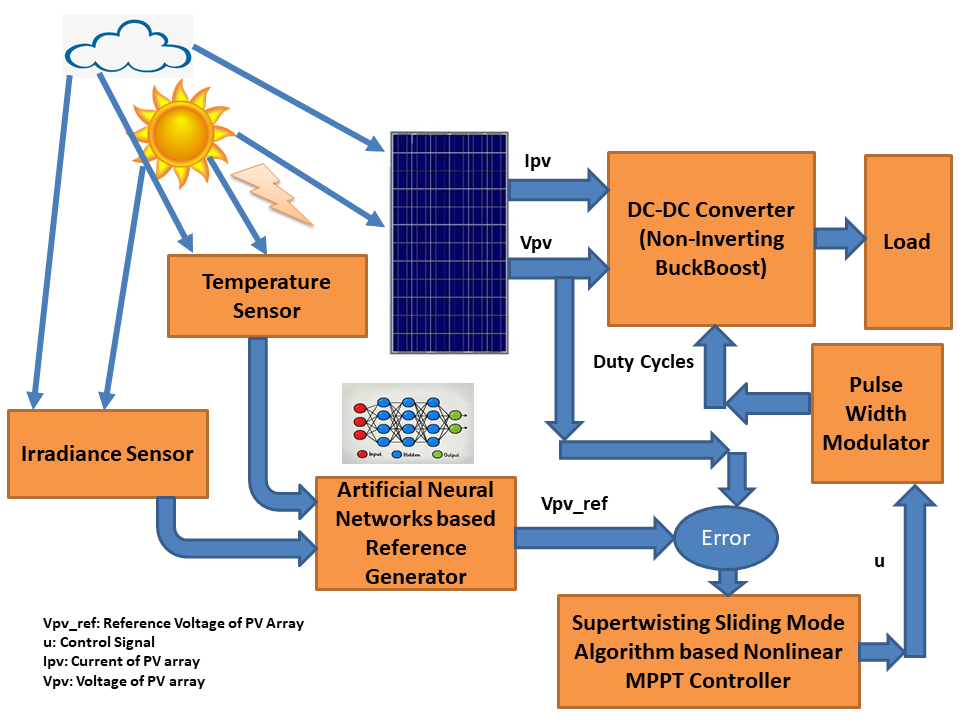
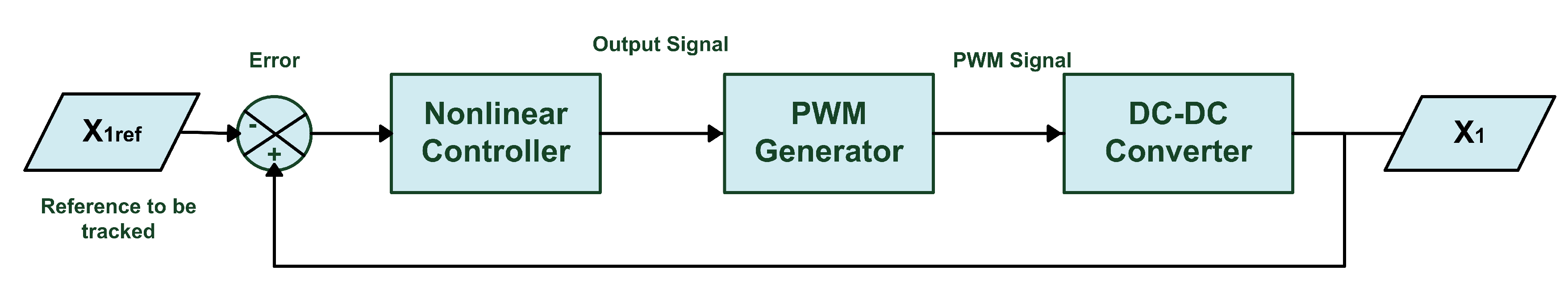
2. Proposed Methodology

The designed nonlinear controller and the conventional MPPT controllers work on different patterns. In conventional controllers, the slope or gradient is constantly being required for achieving the desired MPP and even after achieving the MPP the controller keeps on checking the change in power or the rate of change of slope of PV curve. Nonlinear controller works by first generating the reference voltage $V_{\mathrm{ref}}$ which is to be tracked by the controller in order to achieve the MPP. Each combination of temperature and irradiance gives different characteristic curve of PV array and thus changing $V_{\mathrm{MPP}}$. 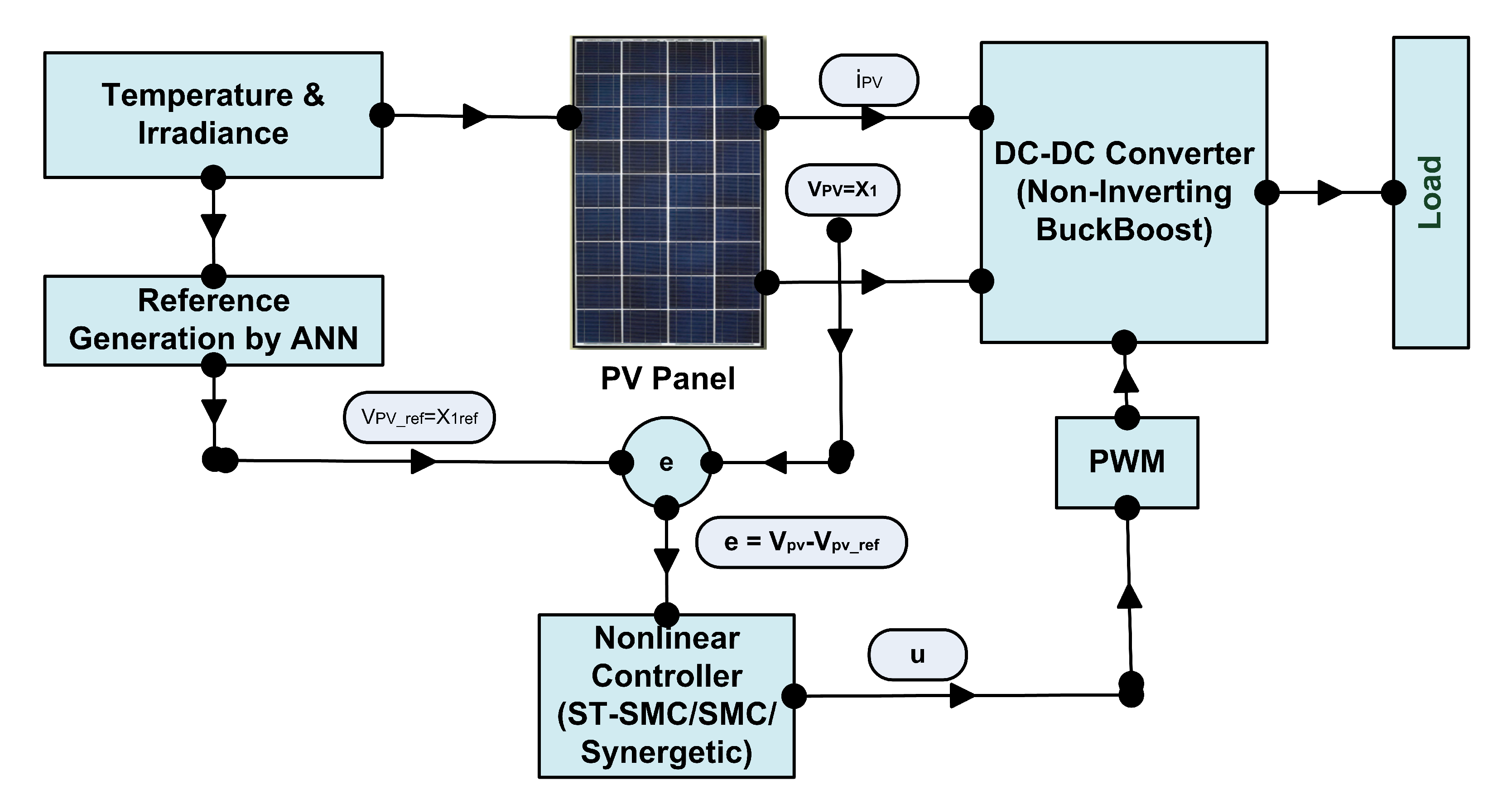Relationship between $V_{\mathrm{MPP}}$ and both irradiance and temperature can be determined by different methods e.g., multiple linear regression method, neuro-fuzzy methods and different artificial intelligence based techniques, etc. In this paper, this relationship is determined by using the application of ANN which produces the reference for peak power voltage. The mathematical model for noninverting Buck-Boost converter is derived which is used for designing a nonlinear controller to track the reference for peak power voltage generated by ANN. The proposed methodology is drawn in Figure 5.

Reference Voltage Generation by ANN

Against each temperature and irradiance value, respective reference voltage is generated which is required to be tracked to ensure the MPPT of PV array. The characteristic curve of PV array changes for each temperature and irradiance. Minute variation in temperature or irradiance can cause change in characteristic curve of PV array which in turn change the maximum power point. Different data sets of $V_{\mathrm{MPP}}$ are prepared for different values of irradiance and temperature. First by keeping the temperature at 25 °C and varying the irradiance from 300 W/m${}^2$ to 4000 W/m${}^2$, different values of $V_{\mathrm{MPP}}$ are obtained. More values of $V_{\mathrm{MPP}}$ are noted by keeping irradiance constant at 1000 W/m${}^2$ and varying the temperature from 17 °C to 55 °C.

There is a need to find the relationship of maximum power point voltage against each temperature and irradiance, for that purpose ANN is used. Feedforward based ANN with three different layers has been used. Those three layers are input layer, hidden layer and an output layer. There are total of six neurons in the hidden layer. In feedforward based ANN, the flow of information is in one direction only. The main objective which is required to be fulfilled efficiently by the use of ANN is to determine the relationship between two inputs and one output. ANN is trained [29] with already obtained data sets of two inputs and one output. The Equation (1) represents the approximation function property of feedforward neural network.

$$f(x,\zeta )=\sum _{i=0}^n{\zeta }_i{\gamma }_i\left(x\right)={\zeta }^T\gamma \left(x\right)$$

(1)

where x is the input vector and in this case there are two inputs which are temperature and irradiance. $\gamma$ = (${\gamma }_0,{\gamma }_1,......,{\gamma }_n{)}^T$ is the vector which represents the basis for nonlinear parameters while the vector $\zeta$ = (${\zeta }_0,{\zeta }_1,......,{\zeta }_n{)}^T$ represents the parameters of the model.

The basis function for nonlinear parameters is defined in Equation (2) in which $w_{im}^{\left(1\right)}$ = $(w_{i0}^{\left(1\right)},w_{i1}^{\left(1\right)},......,w_{in}^{\left(1\right)}{)}^T$ is the vector which contains the weights which are updated during the training of data. k is the activation function which is nonlinear and differentiable. The output of the feedforward neural network is the reference for peak power voltage which can be represented by the generalized output expression of feedforward neural network in Equation (3).

$${\gamma }_i\left(x\right)=k\left(\sum _{m=0}^a{\omega }_{im}^{\left(1\right)}{x}^m\right)$$

(2)

$$y_q(x,\omega )=\sum _{i=0}^n{\omega }_{qi}^{\left(2\right)}{\gamma }_i\left(x\right)=\sum _{i=0}^n{\omega }_{qi}^{\left(2\right)}k\left(\sum _{m=0}^a{\omega }_{im}^{\left(1\right)}{x}^m\right)$$

(3)

The Equation (2) represents the weights and biases of weight vector which shows the links between input and ‘ith’ node of hidden layer. The $w_{qi}^{\left(2\right)}$ with $q=1,...Q$ is the weight vector in Equation (3) which contains the weights and biases for the links between hidden and ‘qth’ node of the output layer.

The parameter vector $\zeta$ is defined in Equation (4) which contains $w^{\left(1\right)}\in$ ${\mathbb{R}}^{a\times n}$ and $w^{\left(2\right)}\in$ ${\mathbb{R}}^{n\times Q}$.

$$\zeta =[{\omega }^{\left(1\right)},{\omega }^{\left(2\right)}]$$

(4)

Neural networks are trained by the given data sets, nonlinear optimization iterative schemes are used by ANN tool to find the parameter $\zeta$ which minimizes the error function of Equation (5).

$${\zeta }^{\tau +1}={\zeta }^{\tau }+▵{\zeta }^{\tau }$$

(5)

The gradient of error function is defined in terms of $▵\zeta$ which is computed by error back propagation method at each iterative step $\tau$. The error function is updated by evaluating the gradient of error function at each iterative step $\tau$. The error function is non convex function of $\zeta$ therefore multiple attempts of optimization algorithm are required to find the best optimal solution.

The Equation (6) represents the expression for reference value of peak power voltage which is obtained by using multiple linear regression method on data sets for comparison with ANN.

$$V_{MPP-Reg}=-1.30987x_1-0.01579x_2+337.74789$$

(6a)

where $x_1$ and $x_2$ represent the data set of temperature and irradiance. While the expression for reference value of peak power voltage given by ANN is represented as general expression in Equation (3) which can also be written as:

$$\begin{array}{cc}\hfill V_{MPP-ANN}=& \sum _{i=0}^n{\omega }_{qi}^{\left(2\right)}{\gamma }_i\left(x\right)\hfill \\ \hfill =& \sum _{i=0}^n{\omega }_{qi}^{\left(2\right)}k\left(\sum _{m=0}^a{\omega }_{im}^{\left(1\right)}{x}^m\right)\hfill \end{array}$$

(6b)

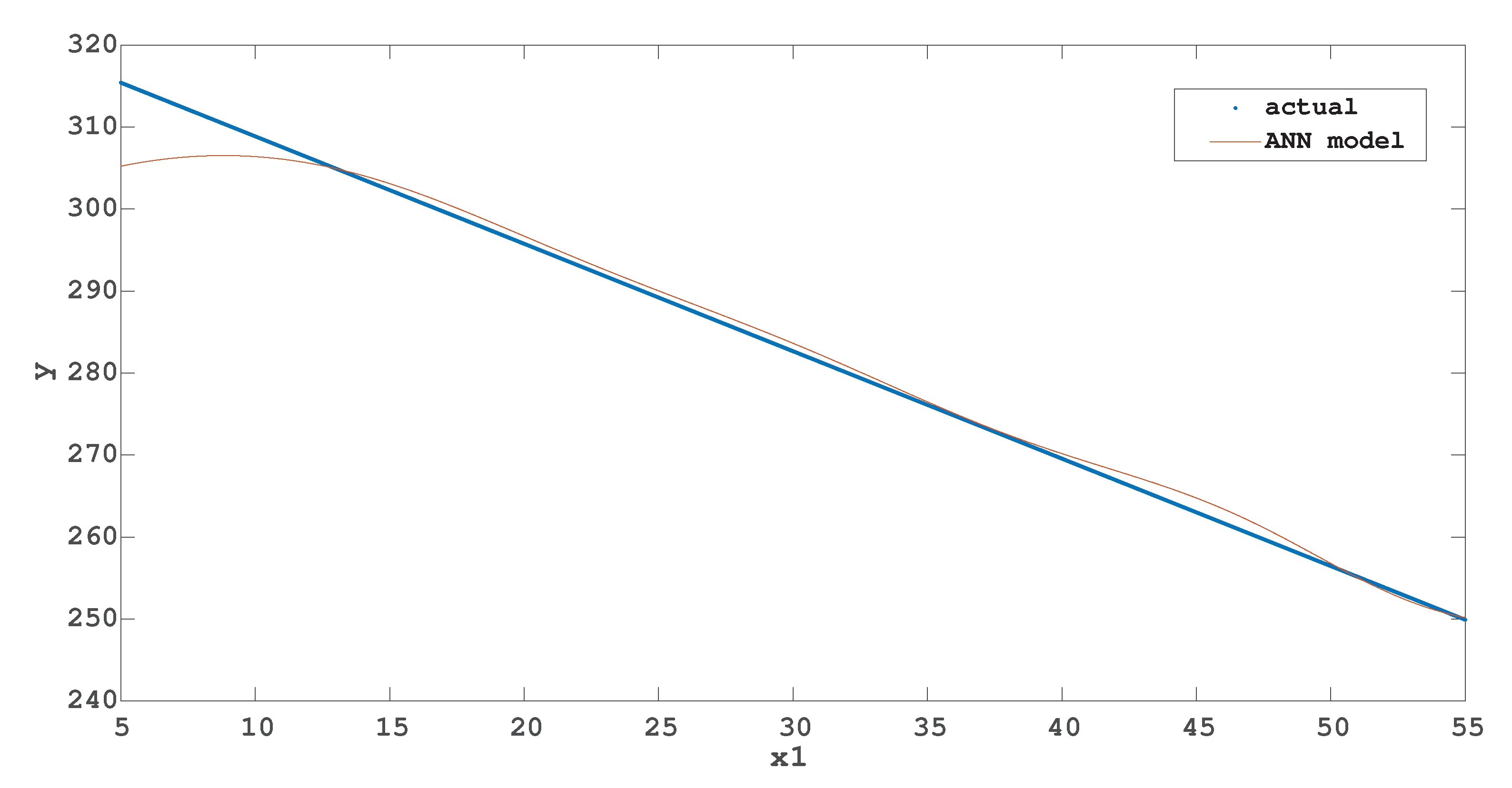
After training, ANN is tested by giving different inputs and then the model predictive output of an ANN is obtained which is compared with an already available model that was obtained by multiple linear regression of the data set. In this comparison, as shown in Figure 6, irradiance is kept constant at 1000 W/m${}^2$ and only temperature is varied for testing the trained ANN model with the one obtained by multiple linear regression algorithm, therefore in Figure 6, only $x_1$ is represented on the x-axis while $x_2$, which is irradiance, is taken as constant for computation of peak power voltage which is the output y of both algorithms.

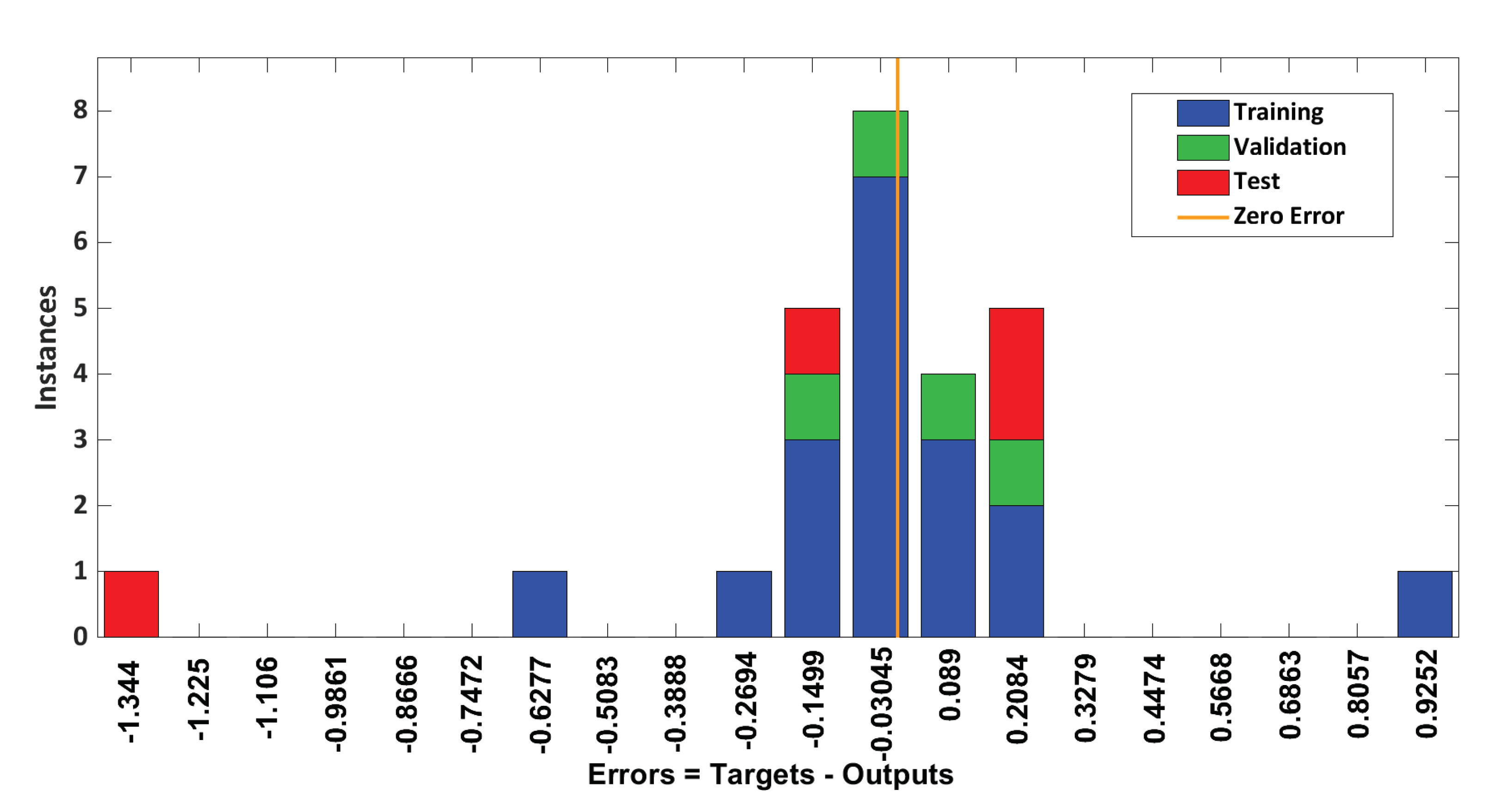
Histogram of an error after training of an ANN is shown in Figure 7.

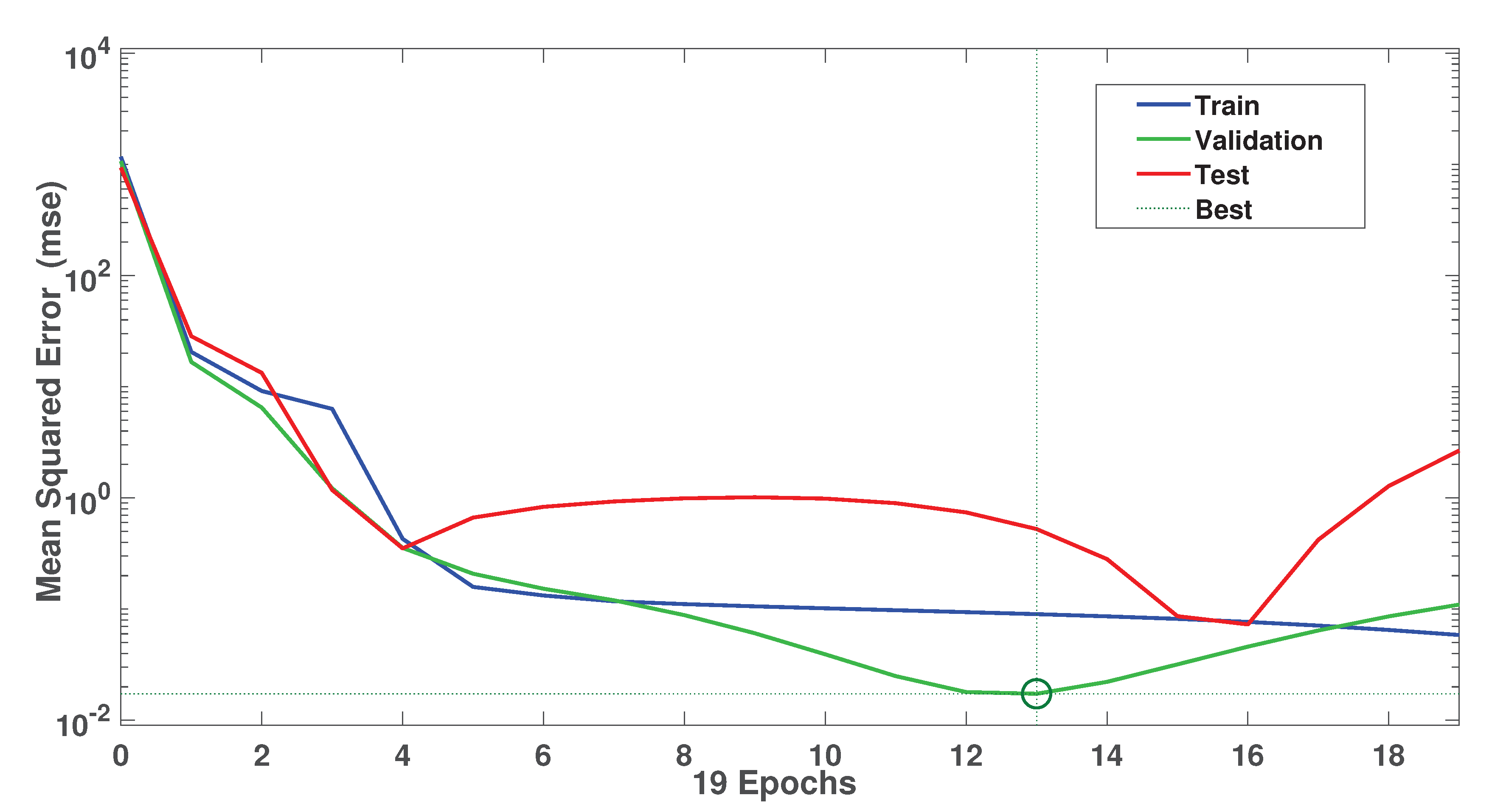
Training, validation and testing phases are shown against the instances of error histogram with a clear indication of zero error.

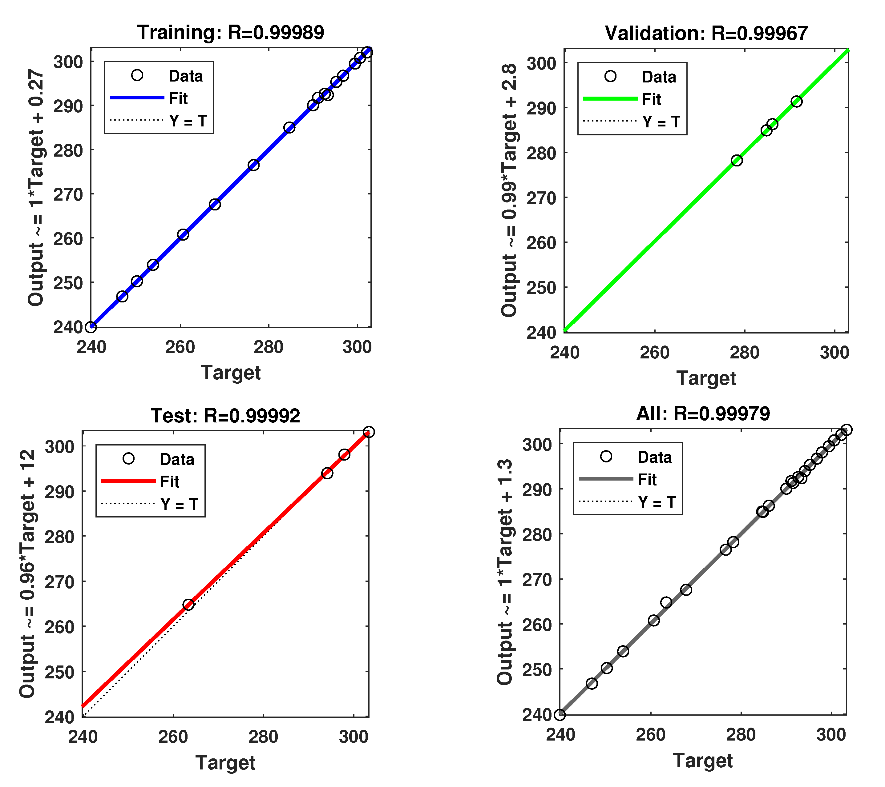
Regression plot of Figure 8 shows somehow a good distribution of data.

The best data fit during the training, validation and testing phases gives the overall best value for coefficient of determination.

Moreover validation performance is shown in Figure 9.

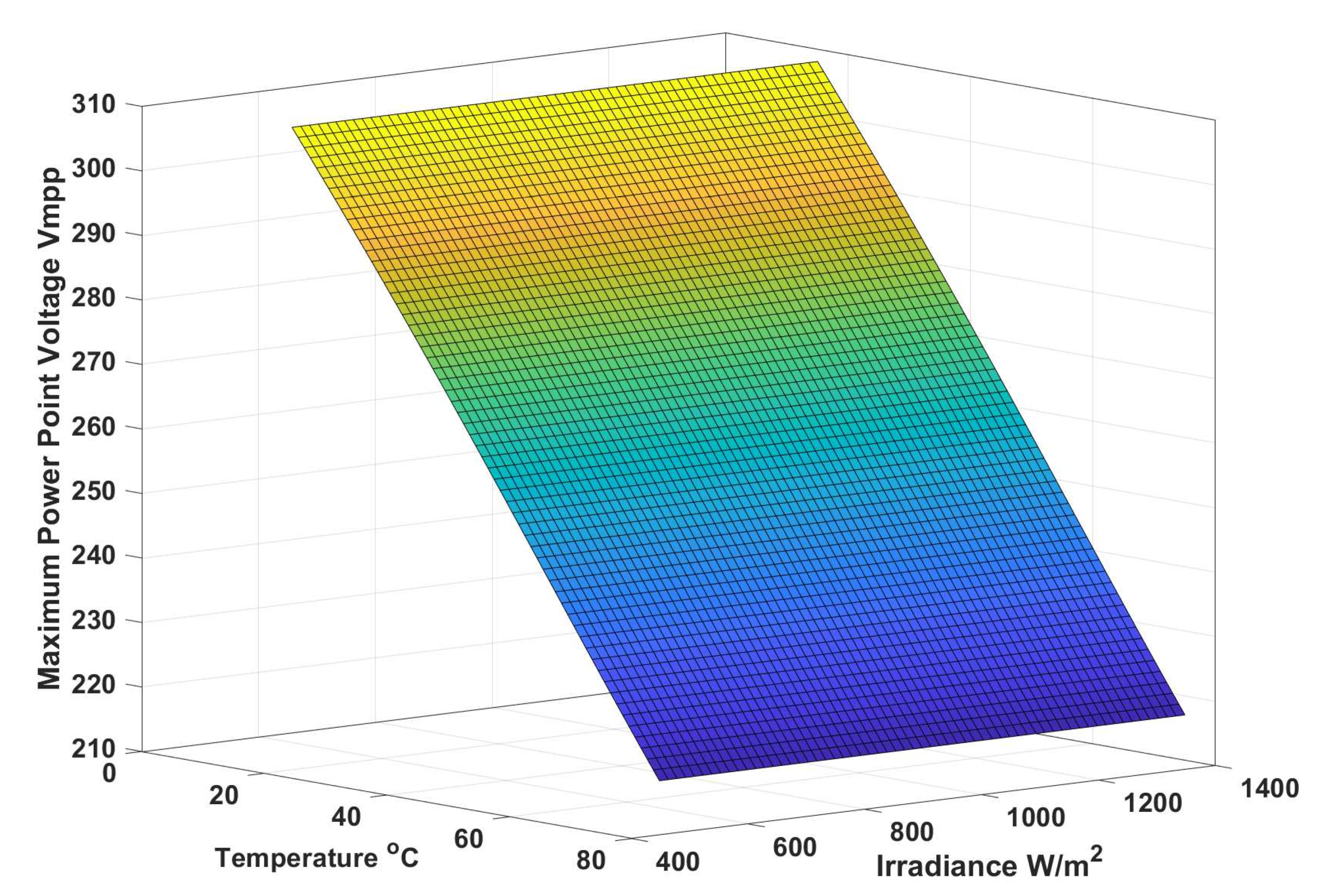
Mean squared error of 19 epochs shows the best validation performance at epoch 13. After deploying the ANN, data points of $V_{\mathrm{MPP}}$ are obtained from ANN model by giving the inputs of temperature and irradiance. The surface plot of Figure 10 shows the relationship of $V_{\mathrm{MPP}}$ against temperature and irradiance.

Figure 11 shows the general flow chart for MPPT control pf PV system. Temperature and irradiance are the two inputs for the reference generation block which computes the reference voltage by using ANN to ensure MPPT. The first error is computed by the difference of reference and actual voltage of PV array. The designed controller takes the error into account and generates the control input to the plant which ensures the perfect tracking of reference voltage of PV. The closed loop system for the MPPT of PV system is shown in Figure 12. The process continues until the error becomes zero.

In our proposed approach, FFNN has been used for reference generation for the peak power voltage and therefore, computational cost would fall into two categories. First is the linear cost which is associated with the computation of sum of weighted inputs of each neuron. The second one is the nonlinear cost which is concerned with the computation of activation functions. The elementary operations for FFNN are computed by fixed-point and floating-point arithmetics. Moreover, the cost for supertwisting sliding mode controller is lower than the other conventional higher order sliding mode controllers due to the absence of derivative of sliding surface in the switching law. The overall cost of our proposed approach is a bit higher than the conventional approaches which makes use of nonlinear controllers along with linear regression techniques for MPPT of PV system. The proposed approach ensures better dynamic performance than those of conventional approaches at the cost of high computations which is no longer an issue due to availability of fast speed processors now a days.

3. Average Mathematical Model

Noninverting Buck-Boost converter shown in Figure 13 can either step-up or step-down the output voltage. For the control of this converter, we require its mathematical model which is derived in this section. The assumption of Continuous Conduction Mode (CCM) holds throughout the paper and for the sake of simplicity, switches and diodes are assumed to be ideal. Further the resistances of inductor and capacitors are also assumed to be negligible and thus taken as zero. The converter has two modes of operations.

Mode1: In this mode both the switches $S_1$ and $S_2$ are closed while both the diodes $D_1$ and $D_2$ are reverse biased. By using Kirchoff’s Laws we have:

$$i_{{\mathrm{C}}_1}=i_{\mathrm{PV}}-i_{\mathrm{L}},$$

(7)

$$i_{{\mathrm{C}}_2}=-\frac{v_{{\mathrm{C}}_2}}{R},$$

(8)

$$v_{\mathrm{L}}=v_{{\mathrm{C}}_1}.$$

(9)

Mode2: In this mode of operation, both the diodes $D_1$ and $D_2$ are forward biased and both switches $S_1$ and $S_2$ are open. Kirchoff’s Laws give:

$$i_{{\mathrm{C}}_1}=i_{\mathrm{PV}},$$

(10)

$$i_{{\mathrm{C}}_2}=i_{\mathrm{L}}-\frac{v_{{\mathrm{C}}_2}}{R},$$

(11)

$$v_{\mathrm{L}}=-v_{{\mathrm{C}}_2}.$$

(12)

Now by using inductor volt second balance and capacitor charge balance, we can write the average model in vector matrix form as:

$$\begin{array}{c}\left[\begin{array}{c}{\dot{v}}_{\mathrm{PV}}\\ {\dot{i}}_{\mathrm{L}}\\ {\dot{v}}_{{\mathrm{C}}_2}\end{array}\right]=\left[\begin{array}{ccc}0& \frac{-u}{C_1}& 0\\ \frac{u}{L}& 0& \left(\frac{u}{L}-\frac{-1}{L}\right)\\ 0& \left(\frac{1}{C_2}-\frac{u}{C_2}\right)& \frac{-1}{R{C}_2}\end{array}\right]\left[\begin{array}{c}{v}_{\mathrm{PV}}\\ i_{\mathrm{L}}\\ v_{{\mathrm{C}}_2}\end{array}\right]\left[\begin{array}{c}\frac{i_{\mathrm{PV}}}{C_1}\\ 0\\ 0\end{array}\right].\end{array}$$

(13)

where u is the input which has to be given in the form of duty cycles to switches $S_1$ and $S_2$ of the converter. Assuming $x_1$, $x_2$, $x_3$ and $\mu$ to be the average values of $v_{{\mathrm{C}}_1}$, $i_{\mathrm{L}}$, $v_{{\mathrm{C}}_2}$ and u respectively, we can write state space equations as:

$$\begin{array}{c}\left[\begin{array}{c}{\dot{x}}_1\\ {\dot{x}}_2\\ {\dot{x}}_3\end{array}\right]=\left[\begin{array}{ccc}0& \frac{-\mu }{C_1}& 0\\ \frac{\mu }{L}& 0& \left(\frac{\mu }{L}-\frac{-1}{L}\right)\\ 0& \left(\frac{1}{C_2}-\frac{\mu }{C_2}\right)& \frac{-1}{R{C}_2}\end{array}\right]\left[\begin{array}{c}{x}_1\\ x_2\\ x_3\end{array}\right]\left[\begin{array}{c}\frac{i_{\mathrm{PV}}}{C_1}\\ 0\\ 0\end{array}\right].\end{array}$$

(14)

The model given in Equation (14) is used in controller design for tracking of MPP.

4. Controller Design

4.1. Supertwisting Sliding Mode Controller

Supertwisting sliding mode control law requires the formulation of an equivalent control along with switching control. For this purpose an appropriate sliding surface has to be designed. Among various surface designing methods, error based designing method is chosen. By taking the error $e_1$ for the first state of the system as:

$$e_1=x_1-x_{1\mathrm{ref}}.$$

(15)

where $x_{1\mathrm{ref}}$ is the reference value for state $x_1$. We can take sliding surface $\sigma$ as follows:

$$\sigma =k_1{e}_1+k_2{x}_2+k_3{x}_3.$$

(16)

Taking time derivative of the Equation (16), we get:

$$\dot{\sigma }=k_1{\dot{e}}_1+k_2{\dot{x}}_2+k_3{\dot{x}}_3.$$

(17)

whereas $k_1$, $k_2$ and $k_3$ are constant design parameters for sliding surface. Similarly, taking the time derivative of Equation (15), we have:

$${\dot{e}}_1={\dot{x}}_1-{\dot{x}}_{1\mathrm{ref}}.$$

(18)

Putting the value of $\dot{e_1}$ in Equation (17), we get:

$$\dot{\sigma }=k_1({\dot{x}}_1-{\dot{x}}_{1\mathrm{ref}})+k_2{\dot{x}}_2+k_3{\dot{x}}_3.$$

(19)

Substituting the values of $\dot{x_1}$, $\dot{x_2}$ and $\dot{x_3}$ from Equation (14) in Equation (19), we have:

$$\begin{array}{cc}\hfill \dot{\sigma }=& k_1\left(\frac{i_{\mathrm{PV}}}{C_1}-\frac{x_2\mu }{C_1}-{\dot{x}}_{1\mathrm{ref}}\right)+k_2\left(\frac{x_1\mu }{L}-\frac{x_3(1-\mu )}{L}\right)\hfill \\ \hfill & +k_3\left(\frac{x_2(1-\mu )}{C_2}-\frac{x_3}{R{C}_2}\right).\hfill \end{array}$$

(20)

For extracting ${\mu }_{\mathrm{equ}}$, we have to put $\sigma =0$ which results in:

$$\begin{array}{cc}\hfill & \frac{-k_1{i}_{\mathrm{PV}}}{C_1}+k_1{\dot{x}}_{1\mathrm{ref}}+\frac{k_2{x}_3}{L}-\frac{k_3{x}_2}{C_2}+\frac{k_3{x}_3}{R{C}_2}=\hfill \\ \hfill & \frac{-k_1{x}_2\mu }{C_1}+\frac{k_2{x}_1\mu }{L}+\frac{k_2{x}_3\mu }{L}-\frac{k_3{x}_2\mu }{C_2}.\hfill \end{array}$$

(21)

${\mu }_{\mathrm{equ}}$ is obtained from Equation (21) which is given as:

$${\mu }_{\mathrm{equ}}=\frac{\frac{-k_1{i}_{\mathrm{PV}}}{C_1}+k_1{\dot{x}}_{1\mathrm{ref}}+\frac{k_2{x}_3}{L}-\frac{k_3{x}_2}{C_2}+\frac{k_3{x}_3}{R{C}_2}}{\frac{-k_1{x}_2}{C_1}+\frac{k_2{x}_1}{L}+\frac{k_2{x}_3}{L}-\frac{k_3{x}_2}{C_2}}.$$

(22)

Switching control ${\mu }_{\mathrm{sw}}$ in case of supertwisting sliding mode design is selected as:

$$\left\{\begin{array}{c}\hfill {\mu }_{\mathrm{sw}}=-a{\left|\sigma \right|}^{\left(0.5\right)}sign\left(\sigma \right)+{\mu }_1,\\ \hfill {\dot{\mu }}_1=-Msign\left(\sigma \right).\hfill \end{array}\right.$$

(23)

where a, $\psi$, ${\mathsf{\Gamma }}_{\min }$, ${\mathsf{\Gamma }}_{\max }$ and M are design parameters which are taken as defined in [30]:

$$M>{\frac{\psi }{\mathsf{\Gamma }}}_{\min }.$$

(24)

$$a^2\ge \frac{4\psi {\mathsf{\Gamma }}_{\max }(M+\psi )}{{\mathsf{\Gamma }}_{\min }^2{\mathsf{\Gamma }}_{\min }(M-\psi )}.$$

(25)

with conditions

$$\psi >|\frac{d\dot{\sigma }}{dt}+\frac{d\dot{\sigma }}{dx}[f(x,t)+b\left(t\right)u\left(t\right)+d\left(t\right)]|.$$

(26)

where $f(x,t)$ is the state matrix, $b\left(t\right)$ is the input matrix and $d\left(t\right)$ is the vector representing the external disturbances occurring in the system.

$$0\le {\mathsf{\Gamma }}_{\min }\le \left|\frac{d\dot{\sigma }}{du}\right|\le {\mathsf{\Gamma }}_{\max }.$$

(27)

The final control law of ST-SMC is given as:

$$\mu =u_{\mathrm{ST}-\mathrm{SMC}}={\mu }_{\mathrm{equ}}+{\mu }_{\mathrm{sw}}.$$

(28)

For the stability of the designed controller, let us consider the Lyapunov candidate function as:

$$V=\frac{1}{2}{\sigma }^2.$$

(29)

Time derivative of Equation (29) yields:

$$\dot{V}=\sigma \dot{\sigma }.$$

(30)

Putting the value of $\dot{\sigma }$ from Equation (20) into Equation (30), we have:

$$\dot{V}=\sigma (k_1{\dot{e}}_1+k_2{\dot{x}}_2+k_3{\dot{x}}_3).$$

(31)

Substituting the values of ${\dot{e}}_1$, ${\dot{x}}_2$ and ${\dot{x}}_3$ from Equations (18) and (14) in Equation (31) yield:

$$\begin{array}{cc}\hfill \dot{V}& =\sigma k_1\left(\frac{i_{\mathrm{PV}}}{C_1}-\frac{x_2\mu }{C_1}-{\dot{x}}_{1\mathrm{ref}}\right)+\sigma k_2\left(\frac{x_1\mu }{L}-\frac{x_3(1-\mu )}{L}\right)\hfill \\ \hfill & +\sigma k_3\left(\frac{x_2(1-\mu )}{C_2}-\frac{x_3}{R{C}_2}\right).\hfill \end{array}$$

(32)

Now by putting the value of $\mu$ from Equation (28) in Equation (32), we get:

$$\dot{V}=\sigma \left(-k_1{\left|\sigma \right|}^{0.5}sign\left(\sigma \right)-k_2\int sign\left(\sigma \right)d\left(\tau \right)\right).$$

(33)

Simplification of Equation (33) gives the following expression for $\dot{V}$ as:

$$\dot{V}=-k_1{\left|\sigma \right|}^{1.5}-k_2\sigma \int sign\left(\sigma \right)d\left(\tau \right).$$

(34)

Since the derivative of the Lyapunov function is negative definite, it ensures the global asymptotic stability of the proposed controller. Parameters M and a are chosen according to the bounds given in Equations (24) and (25) such that $\dot{V}$ always remains negative definite.

4.2. Sliding Mode Controller

SMC is designed using the same ${\mu }_{\mathrm{equ}}$ used in supertwisting sliding mode control design. The difference between the two techniques is the switching control which in case of conventional SMC is given as:

$$u_{\mathrm{sw}}=-ksign(\sigma /\nu ).$$

(35)

where $\nu$ is used to minimize the chattering effect. Hence the sliding mode control law is given as:

$$u_{\mathrm{smc}}={\mu }_{\mathrm{equ}}+u_{\mathrm{sw}}.$$

(36)

4.3. Synergetic Controller

For synergetic control law, only one macro variable is selected due to the presence of one control input. The purpose of this control is to track the state variable to its desired value with an exponential rate. The dynamic evolution is thus considered as:

$$T\dot{\sigma }+\sigma =0.$$

(37)

where T is a positive number and represents the convergence rate. Now by putting the values of $\dot{\sigma }$ and $\sigma$ from Equations (19) and (16), respectively in Equation (37), on simplification we get:

$$\begin{array}{cc}\hfill \frac{-\sigma }{T}=& \left(-\frac{k_1{i}_{\mathrm{PV}}}{C_1}+\frac{k_1{x}_3}{L}-\frac{k_3{x}_2}{C_2}+\frac{k_3{x}_3}{R{C}_2}+K_1{\dot{x}}_{1\mathrm{ref}}\right)\hfill \\ \hfill & \left(-\frac{k_1{x}_2}{C_1}+\frac{k_2{x}_1}{L}+\frac{k_2{x}_3}{L}-\frac{k_3{x}_2}{C_2}\right){\mu }_{\mathrm{sc}}.\hfill \end{array}$$

(38)

We get the required control input $\mu$ = ${\mu }_{\mathrm{sc}}$ as:

$${\mu }_{\mathrm{sc}}=\frac{\frac{-\sigma }{T}-\frac{k_1{i}_{\mathrm{PV}}}{C_1}+\frac{k_1{x}_3}{L}-\frac{k_3{x}_2}{C_2}+\frac{k_3{x}_3}{R{C}_2}+K_1{\dot{x}}_{1\mathrm{ref}}}{-\frac{k_1{x}_2}{C_1}+\frac{k_2{x}_1}{L}+\frac{k_2{x}_3}{L}-\frac{k_3{x}_2}{C_2}}.$$

(39)

For the stability of proposed controller, the value of $\dot{\sigma }$ from Equation (37) is substituted in Equation (30) to get:

$$\dot{V}=\frac{-{\sigma }^2}{T}.$$

(40)

or

$$\dot{V}=\frac{-2V}{T}.$$

(41)

The Equations (40) and (41) show that the derivative of Lyapunov function is negative definite and the designed controller is globally exponentially stable.

5. Simulations and Results

The performance of the proposed controllers given by Equations (28), (36) and (39) is validated using the MATLAB/Simulink environment. The parameters of the proposed controllers have been given in

Table 1. Parametric values of the controllers.

Controller	Parameters	Values
Supertwisting sliding mode controller	M	0.5
	a	500
Sliding Mode controller	k	5
	$\nu$	0.5
Synergetic controller	$k_1$	9
	$k_2$	43.8
	$k_3$	0.0012
	T	0.0012

. There are different methods for choosing the optimal values of gains of the controller like machine learning based algorithms, ANN, optimization-based techniques, etc. In this work, we used hit and trial method for selecting the gain values of the controller to get the desired response, whereas, the values of ‘M’ and ‘a’ are selected according to Equations (24) and (25). The electrical components of converter are listed in

Table 2. Parameters of converter.

Parameter	Value
Inductor, L	11 mH
Input Capacitor, $C_1$	67 $\mathsf{\mu }$F
Output Capacitor , $C_2$	480 $\mathsf{\mu }$F
Load resistor, R	20 $\mathsf{\Omega }$
Switching frequency, $f_{\mathrm{s}}$	100 KHz

. The values of these components are selected which operate the converter in CCM. Forward voltage drop and switching losses of power electronics switches have to be accounted for testing the controller in realistic environment. These factors introduce power loss in the controller. The proposed controllers do not take these losses into account because the control laws for proposed controllers are derived by assuming the ideal operation of the converter.

Table 3. Parameters of PV array.

Parameter	Value
Series-connected modules per string	10
Parallel strings	1
Voltage at maximum power point, $V_{\mathrm{MPP}}$	290 V
Current at maximum power point, $I_{\mathrm{MPP}}$	7.35 A
Open circuit voltage, $V_{\mathrm{OC}}$	36.3 V
Short circuit current, $I_{\mathrm{SC}}$	7.84 A
Maximum Power	213.15 W

contains the parameters of PV array.

The proposed controllers are validated under different environmental conditions to get their different responses at different operating conditions; therefore this section is divided into different subsections. The first subsection contains the simulations of the proposed ST-SMC under changing irradiance. The second subsection contains the performance of ST-SMC under changing temperature. Comparison of ST-SMC with synergetic and sliding mode controllers under changing temperature and irradiance is given in the third subsection. The comparison of the existing controllers and the proposed controller is discussed in the fourth subsection.

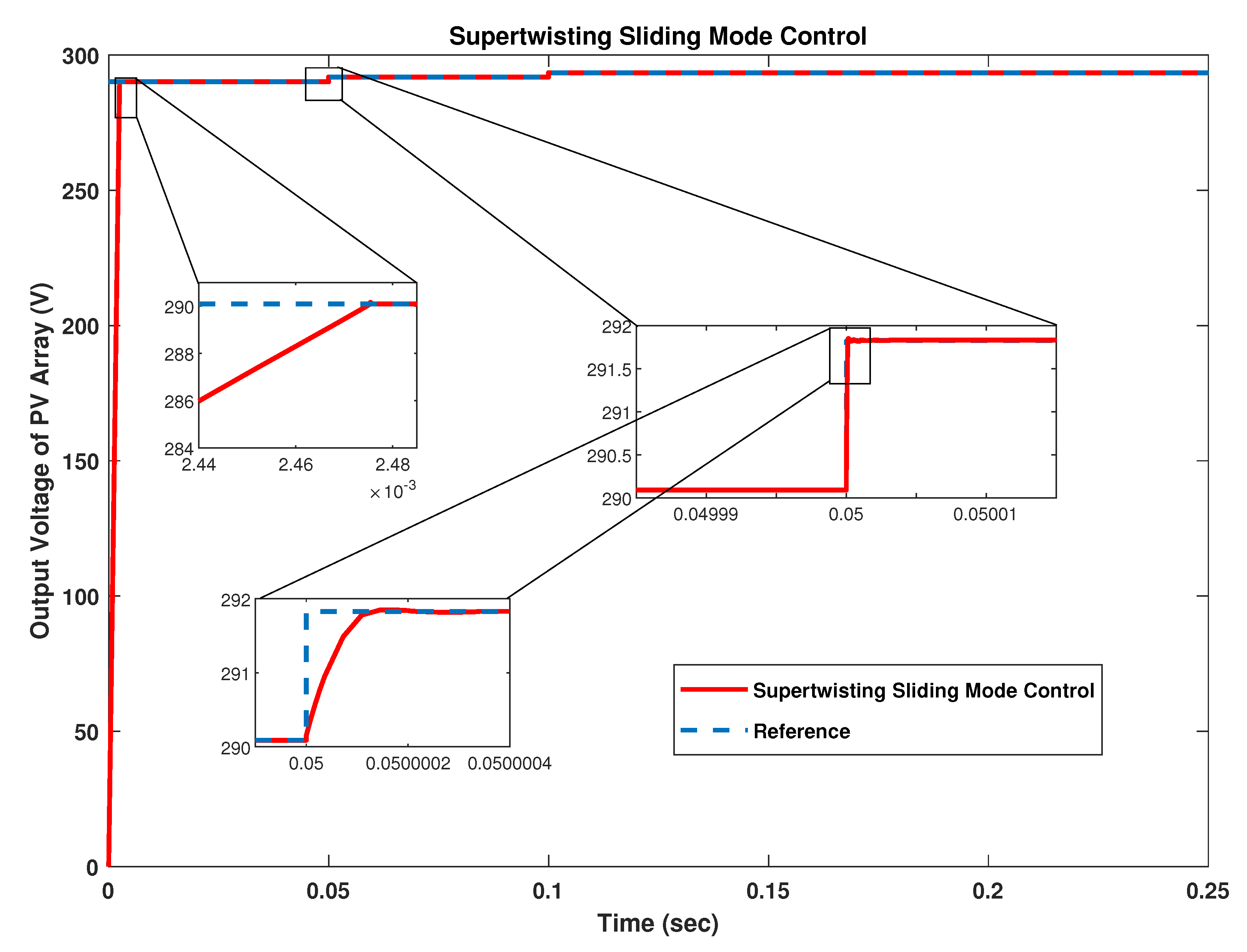
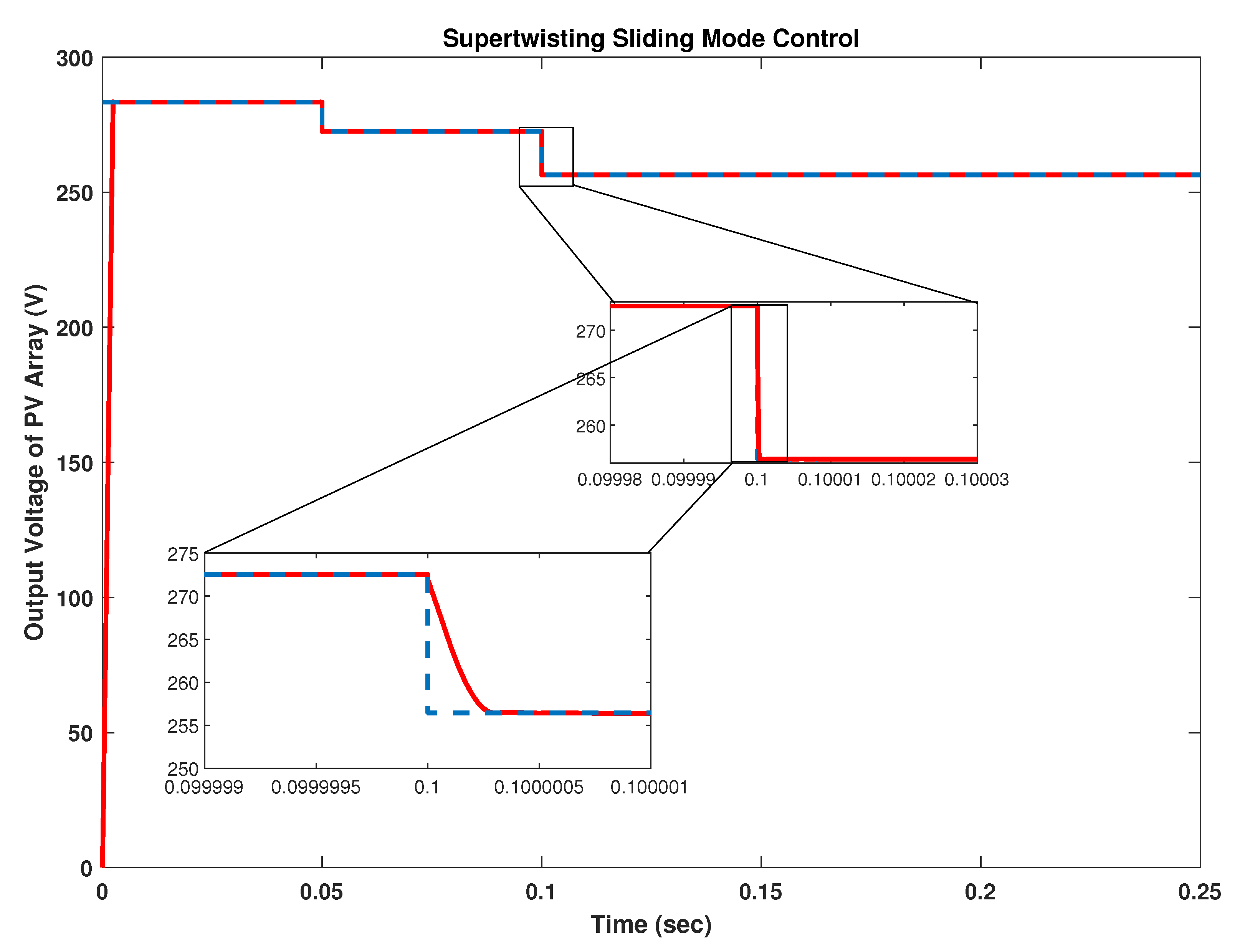
5.1. Response of ST-SMC under Changing Irradiance

The irradiance level is first maintained at a standard level of 1000 W/m${}^2$ and is changed to 850 W/m${}^2$ and then to 700 W/m${}^2$ with a regular interval of 0.05 s. The temperature of 25 °C is maintained throughout the process. The response of output voltage of the PV array under changing irradiance is shown in Figure 14.

The reference for peak power voltage depends upon the change in irradiance and temperature. The controller successfully tracks the reference peak power voltage generated by the application of ANN with almost zero steady state error. This also shows the robustness of designed controller under the environmental variations which are change in temperature and irradiance. The settling time is 2.4 ms and there is no undershoot in the dynamic response, however there is negligibly small overshoot of 0.0415 V in this case. The rise time of ST-SMC is 2.0 ms.

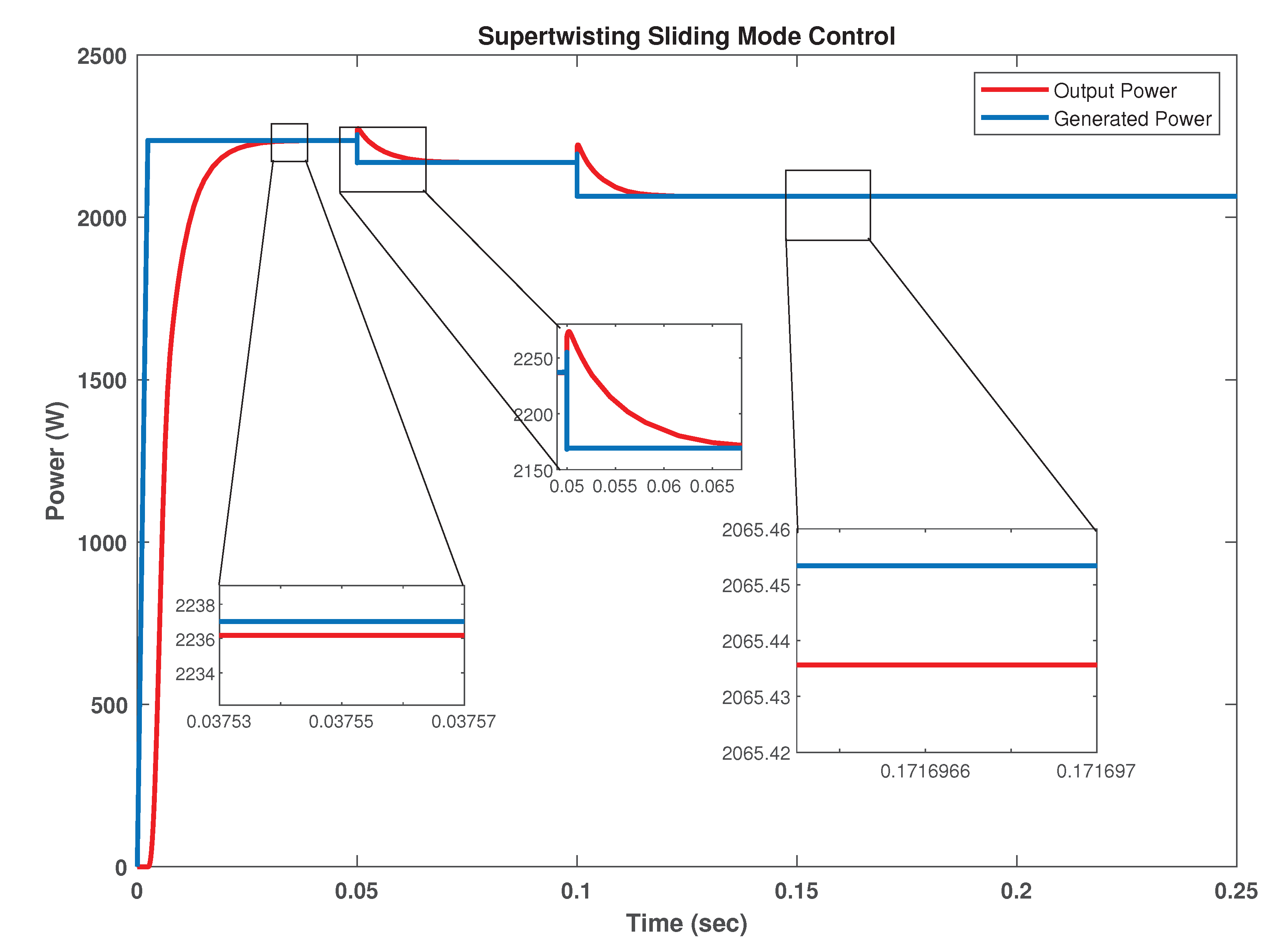
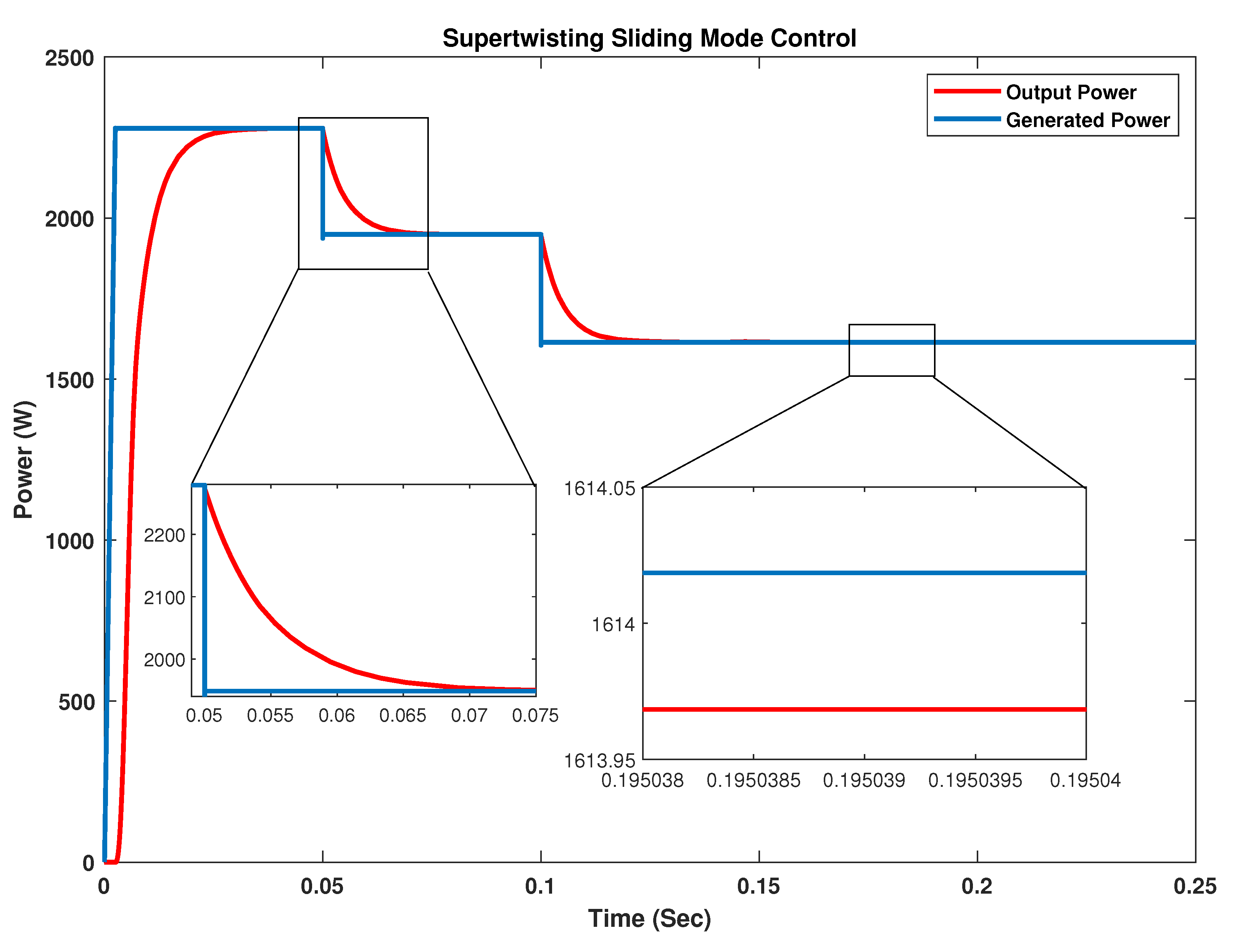
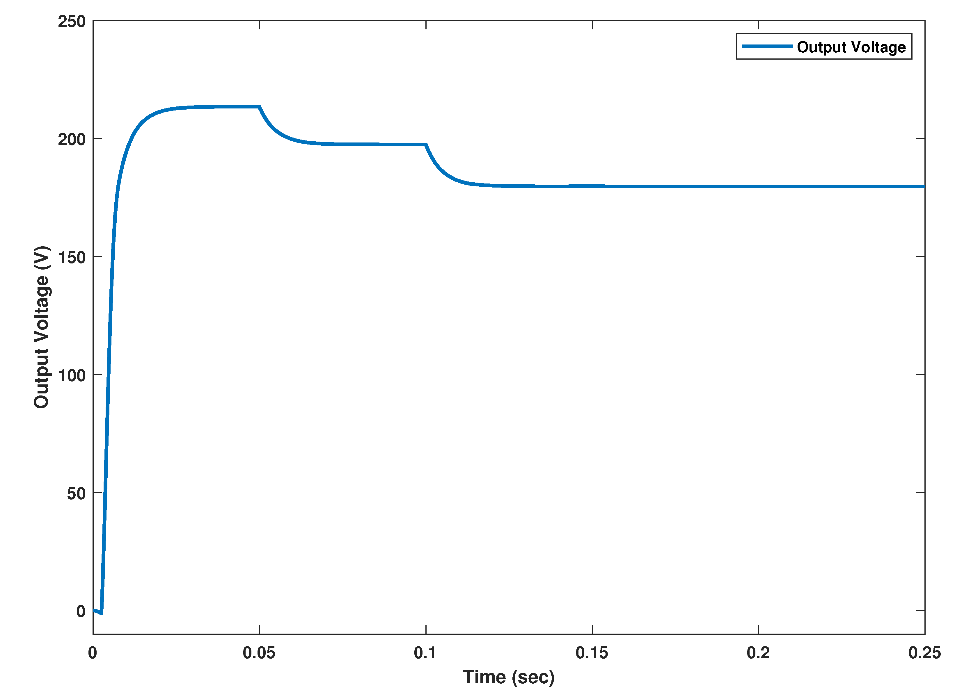
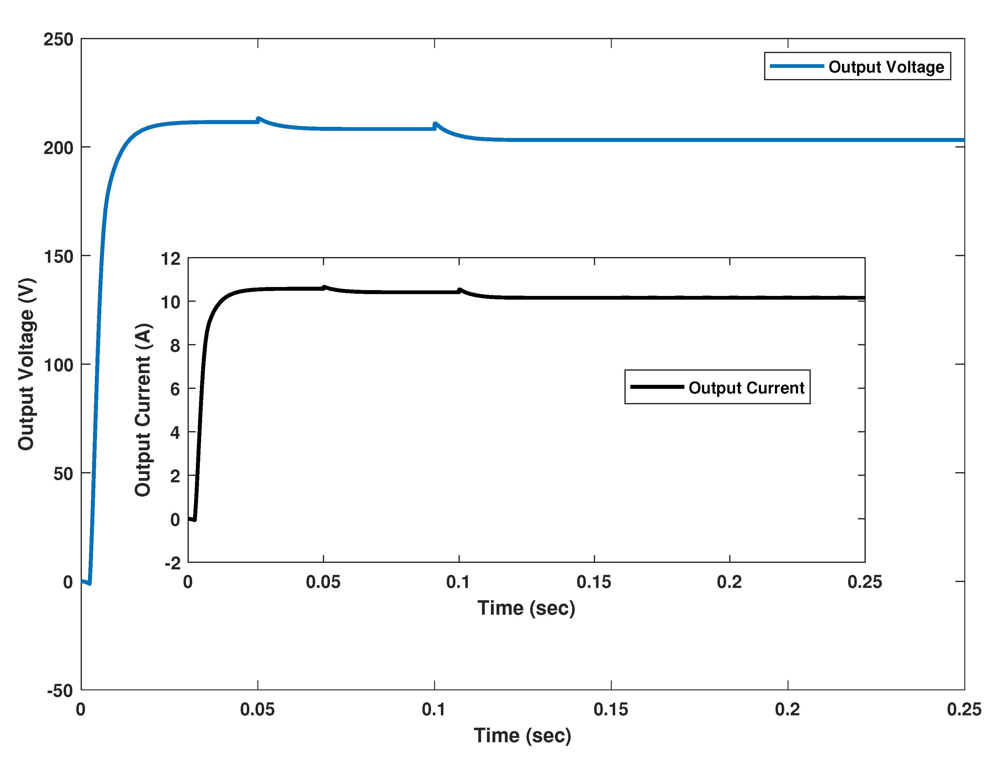
Variations in irradiance level also affect the generated power and the power produced at the output. The response of power under these variations is depicted in Figure 15. The MPP is achieved within 2.5 ms with no steady state error and oscillations/ripples in steady state response is observed. Furthermore, maximum power is successfully transferred by the converter with more than 97% efficiency. The voltage and current at the output side of the converter is shown in Figure 16.

5.2. Response of ST-SMC under Changing Temperature

In this subsection, the response of ST-SMC is validated by varying the temperature at regular intervals of 0.05 s. The temperature is first maintained at 30°C and is varied to 38 °C and then to 50 °C. The irradiance level in this case is kept constant at 1000 W/m${}^2$. The response of PV output voltage under changing temperature has been shown in Figure 17. It can be seen that even at the time of change in temperature, the controller perfectly tracks the reference peak power voltage with no undershoot and negligible overshoot of 0.0383 V. There is a rise time of 0.0019 s and settling time of 2.4 ms. The controller exhibits a better tracking of the reference voltage for extracting the maximum power from the PV panel. The variation in temperature changes the reference peak power voltage and thus power changes accordingly. The variation in power (generated and output) with respect to temperature variations are shown in Figure 18. The tracking is achieved in 1.65 ms with no oscillations/ripples and zero steady state error. The efficiency observed is again more than 95%. Output voltage and current of the converter are shown in Figure 19.

5.3. Comparison of ST-SMC with Synergetic and Sliding Mode Controllers under Changing Temperature and Irradiance

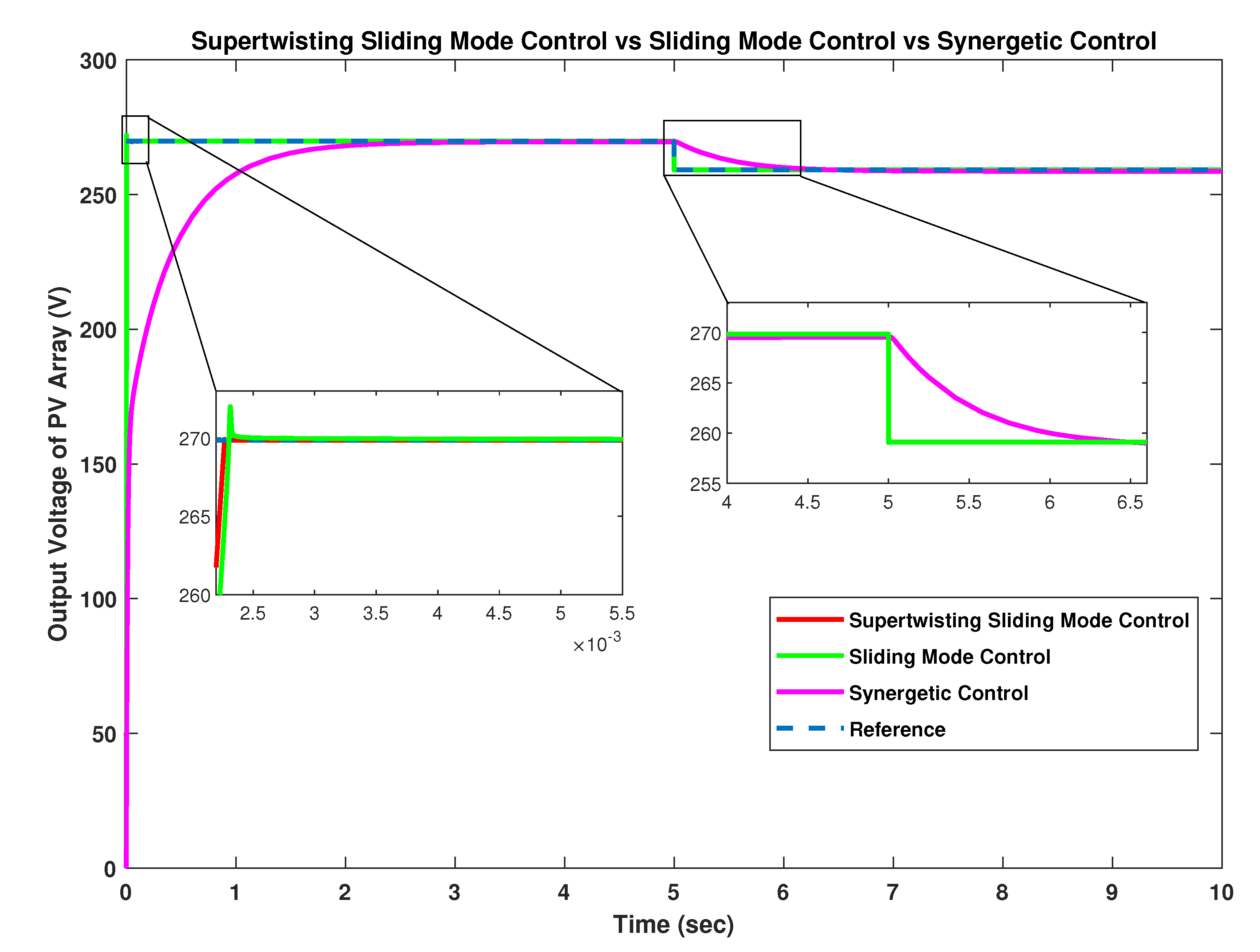
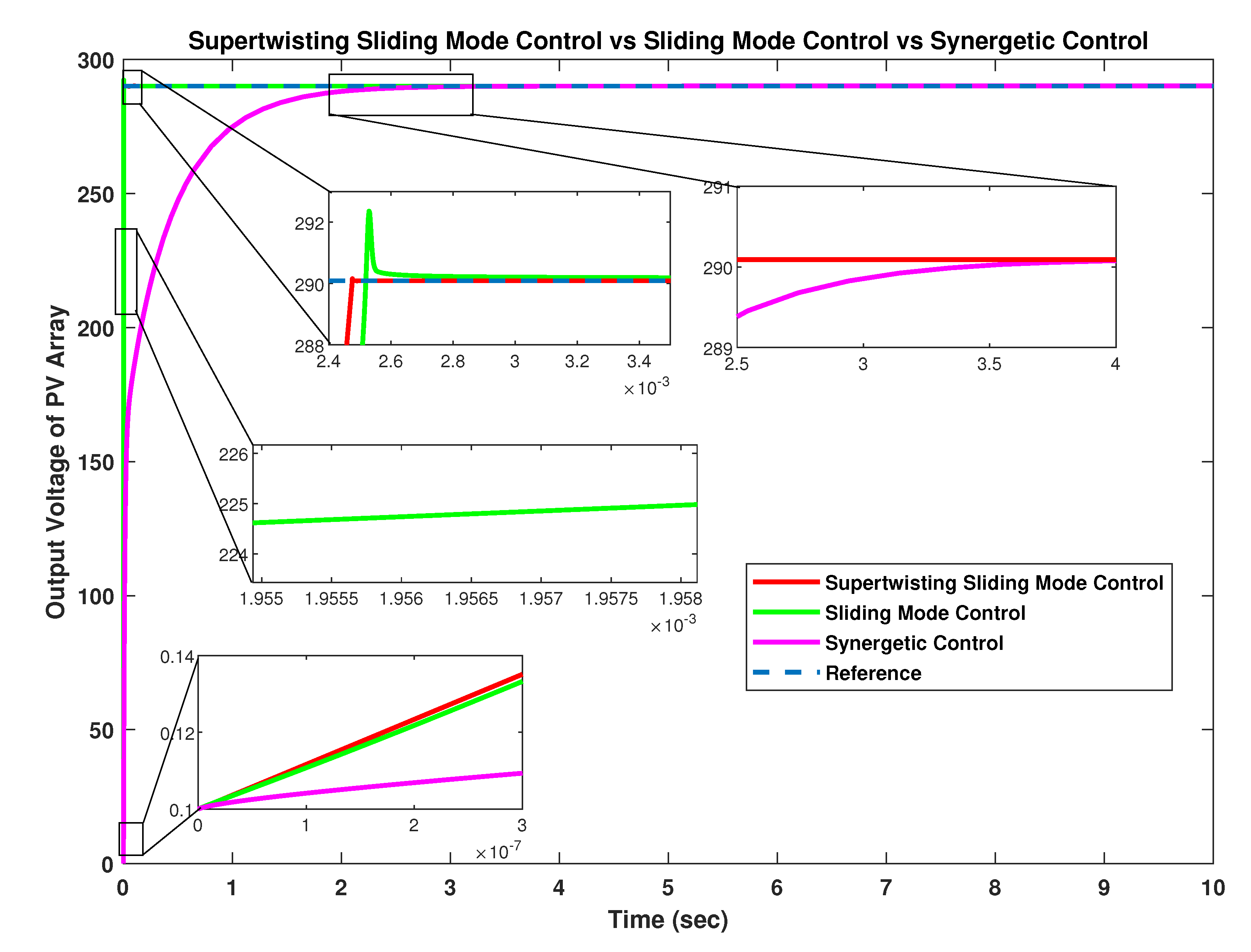
Figure 20 shows the comparison of the proposed controllers at standard temperature and irradiance level (25 °C, 1000 W/m${}^2$). It can be seen that there is an overshoot of 0.7789 V in the case of SMC while ST-SMC shows a negligible overshoot of 0.0415 V. Synergetic controller on the other hand shows lesser overshoot of 0.0042 V but it has delayed convergence when compared to both ST-SMC and SMC.

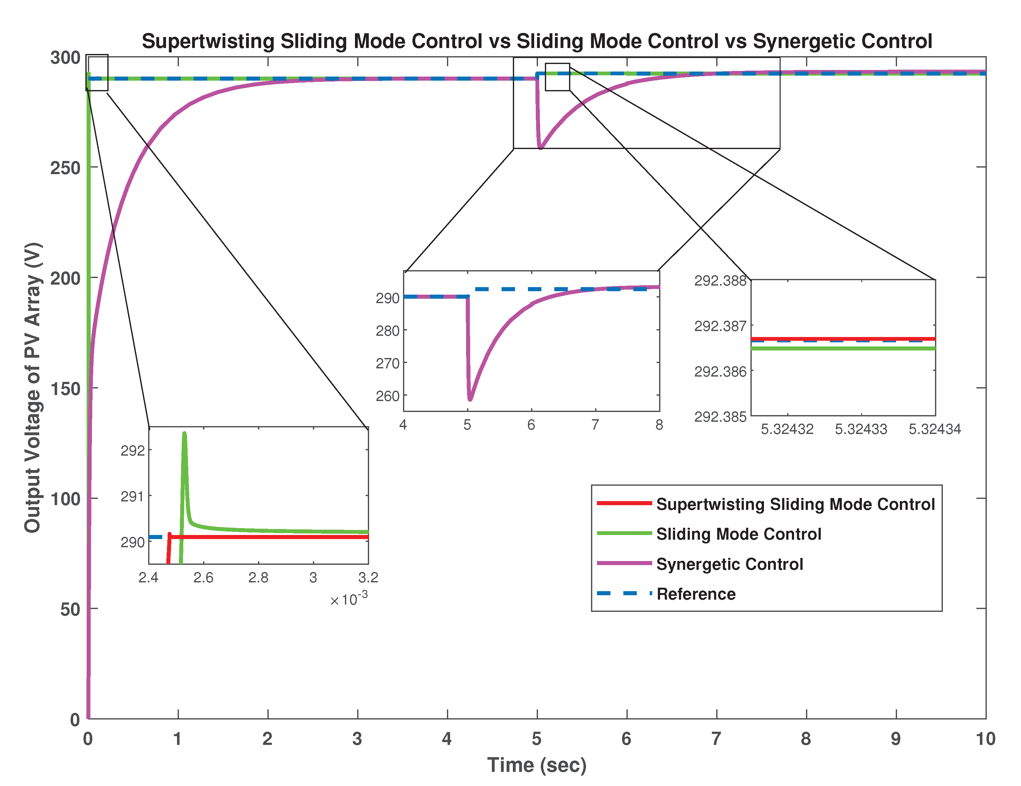
The comparison of all proposed controllers under changing irradiance levels has also been done in Figure 21 where temperature is kept constant at 25 °C. It has been observed that when irradiance level is decreased from 1000 W/m${}^2$ to 800 W/m${}^2$, both ST-SMC and SMC show robustness against the variations, however ST-SMC still has a faster convergence rate than SMC. The synergetic controller on the other hand is not robust like ST-SMC and SMC which shows a big undershoot in the case of changing irradiance level. The settling time for synergetic controller is 1.4767 s. In addition, the settling time for ST-SMC is 0.0024 s which is less than that of 0.0025 s for SMC. Moreover, SMC shows a steady state error of 2.2596 V, whereas both ST-SMC and synergetic controller show almost zero steady state error.

Comparison of proposed controllers under changing temperature has been shown in Figure 22 where temperature is changed from 40 °C to 48 °C by keeping the irradiance constant at 1000 W/m${}^2$. ST-SMC has an overshoot of 0.0406 V while SMC shows an overshoot of 0.8140 V. The overshoot is almost zero for synergetic controller. At the time of temperature change, both ST-SMC and SMC show robustness against the change while a delayed convergence is observed for synergetic controller. SMC shows the steady state error of 2.1961 and no steady state error is observed for the case of ST-SMC and synergetic control.

5.4. Comparison between Proposed and Other Nonlinear Controllers

In this subsection, comparison between the proposed nonlinear controllers and the recently proposed nonlinear controllers [25] has been made. The values of dynamic performance are listed in

Table 4. Comparison of controllers.

Response	P&O	FLBC	BS	IBS	Synergetic	SMC	ST-SMC
Rise Time (ms)	2.22	2.17	2.42	2.17	685.9	2.00	2.00
Settling Time (ms)	NA	8.4	3.8	3.2	1476.7	2.5	2.4
Overshoot (V)	74	15.4	0	13.94	0.0042	0.7789	0.0415
Steady State Error (V)	6	0.5	1	0	0	2.2596	0

where proposed nonlinear controllers are compared with respect to their rise time, settling time, overshoot, undershoot and steady state error under standard temperature of 25 °C and an irradiance of 1000 W/m${}^2$.

In terms of rise time, it can be seen that both SMC and ST-SMC have same value of 2.00 ms which is better than all the listed controllers in [25]. The rise time of synergetic controller is very large (0.6 s) when compared with all the listed controllers. The settling time of ST-SMC is 2.4 ms while that of SMC is 2.5 ms. The settling time for synergetic controller is 1.4 s which shows the late convergence to reference voltage when compared to all other controllers. ST-SMC has the fastest rate of convergence when compared to all other controllers.

There is no overshoot in the response of backstepping (BS), while a very little overshoot of 0.0042 V is present in the response of synergetic controller. The overshoot of ST-SMC is 0.0415 V which is also negligible when compared to others. SMC has significant overshoot of 0.7789 V while all other controllers have larger overshoots present in them.

Further, almost all three controllers i.e., IBS, synergetic and ST-SMC have almost zero steady state error. The steady state error in case of SMC is 2.2596 V while all other controllers have significant steady state errors. Moreover chattering and oscillations are negligible in case of ST-SMC while the response of other nonlinear controllers shows oscillations.

In a nutshell, after comparison of all the proposed controllers from the simulations under varying temperature and irradiance, it can be concluded that ST-SMC is the best choice for MPPT of PV array system using Buck-Boost DC-DC converter when it is required to track the reference voltage with no chattering even in the presence of disturbance which is changing environmental conditions in our case.

6. Conclusions and Future Work

Getting maximum power from a PV system with negligible loss under changing environmental conditions is an on-going challenge. In this paper ST-SMC is designed, which not only resolves the problem of chattering but also enhances the overall dynamic response of the system. Artificial neural networks, which are trained using the data sets obtained from the characteristic curves of a PV array, are used to generate peak power voltage as a reference by taking temperature and irradiance as an input. The reference generated by ANN is then tracked by nonlinear controller using Buck-Boost DC-DC converter. Along with ST-SMC, synergetic and sliding mode controllers are also presented to meet the control objectives and for comparison with ST-SMC. The overall performance of proposed nonlinear controllers is simulated under changing environmental conditions and the performance of ST-SMC is compared with the other proposed nonlinear controllers given in literature. It is established that ST-SMC shows the overall better dynamic response while meeting all the control objectives with negligible chattering and oscillations. Global asymptotic stability of a system is ensured using Lyapunov stability criterion.

In the future, this work can be extended by further enhancing the accuracy of reference generation using different deep learning based algorithms and their combination with other artificial intelligence based techniques for efficient MPPT of PV systems.