Metamodeling for Uncertainty Quantification of a Flood Wave Model for Concrete Dam Breaks

Abstract

Uncertainties in instantaneous dam-break floods are difficult to assess with standard methods (e.g., Monte Carlo simulation) because of the lack of historical observations and high computational costs of the numerical models. In this study, polynomial chaos expansion (PCE) was applied to a dam-break flood model reflecting the population of large concrete dams in Switzerland. The flood model was approximated with a metamodel and uncertainty in the inputs was propagated to the flow quantities downstream of the dam. The study demonstrates that the application of metamodeling for uncertainty quantification in dam-break studies allows for reduced computational costs compared to standard methods. Finally, Sobol’ sensitivity indices indicate that reservoir volume, length of the valley, and surface roughness contributed most to the variability of the outputs. The proposed methodology, when applied to similar studies in flood risk assessment, allows for more generalized risk quantification than conventional approaches.

1. Introduction

Safety standards applied to large dams must be maintained at a high level to provide sufficient protection for the downstream population. The safety standards are normally based on three pillars: thorough design, systematic monitoring, and emergency concept [1]. A dam is normally designed by evaluating its performance in all possible operational conditions (including maximum loads), whereas monitoring aims to detect structural defects or external threats to dam safety so that certain safety measures can be taken. Finally, the emergency concept aims to minimize the degree of potential consequences of the dam failure, and in some countries (e.g., Switzerland) it is included in measures of civil protection [2,3]. To help the decision-making process within the emergency concept, risk is commonly assessed by using a computational model of a potential dam break. Three essential steps of such an assessment are: (i) the simulation of the outflow hydrograph resulting from the dam break, (ii) the propagation of this hydrograph in the downstream topography, and (iii) the estimation of loss of life (LL). This study moves toward the estimation of LL due to a dam-break by focusing on the assessment of the flow quantities reached downstream of the dam in case of its failure, addressed through the aforementioned first two steps.

In this study, a risk assessment for the first two steps mentioned above was performed for hydropower dams in Switzerland, which is a country with one of the highest densities of dams in the world (five per 1000 km² [1]). To reflect the risk level potentially associated with the Swiss hydropower infrastructure, the population of hydropower dams that are representative for the country was considered. About 90% of hydroelectricity in Switzerland is supplied by large dams, according to the International Commission on Large Dams definition [4]. However, large dams account for only 14% of all hydropower plants in the country. This explains the high importance of each large dam. Among different dam types, concrete arch dams have the largest share of Swiss hydroelectricity production (45%), followed by gravity (39%) and embankment (11%) dams [5]. Based on this, the geometry of a large concrete arch dam was chosen for this study as a proxy for large hydropower dams in Switzerland. To obtain the largest possible discharge values, the tallest third of these dams was considered (over 100 m in height); to model the worst-case scenario, the failure mode was assumed to be complete and instantaneous. The latter is also a common assumption for concrete dams [6], supported by the knowledge about past failures of concrete arch dams (e.g., the Malpasset dam in France; the Idbar dam in former Yugoslavia; the Moyie dam in USA [7]).

To evaluate the flow quantities downstream of the dam after its failure, first the quantity of water released from the reservoir needs to be estimated. Empirical and analytical methods, which are commonly used for this purpose, calculate the flow quantities (e.g., the peak outflow and the time to the peak outflow) by applying regression equations to historical or experimental observations [8]. However, these approaches are usually not able to fully reproduce flood wave dynamics and only provide results in coarse spatial and temporal resolution [9]. Therefore, in this study a hydrodynamic model was applied to simulate detailed flood wave dynamics. The model simulates water flow by solving equations of the underlying physical processes. The result not only provides the outflow hydrograph, but also routes this hydrograph through the downstream area to the final receptor [10]. An advantage of this computational method is its ability to solve time-dependent and multi-dimensional problems, whereas its drawback is the high complexity resulting in the increased uncertainty in model parameters (elaborated in Section 2.3.1).

The presence of numerous uncertainties in the computational models used for dam risk assessment (e.g., uncertain model inputs, uncertainty due to high complexity of the model) and the importance of addressing these has been recognized in numerous studies conducted in the field of dam safety [11]. Until now, the analysis of uncertainty in this field was mainly performed in a qualitative manner e.g., [12]. Quantitative estimation of uncertainties has mainly focused on embankment dam failures, which commonly gradually fail and enable datasets with historical observations to be established; these datasets were analyzed with regression methods or Monte Carlo (MC) simulations to build probability distributions and quantify uncertainties in the discharge or parameters of the breach e.g., [13].

As for instantaneous dam-break flood models, which are the focus of this study, the application of regression and MC approaches based on historical datasets is limited. The reason is the lack of recorded observations (e.g., water depth or velocity reached downstream) for instantaneous failures due to their nature. Alternatively, for hydrodynamic models simulating the dam-break flood wave, available computational power enables running a sufficient number of model realizations for MC to be applied to the shallow water equations (SWEs). Furthermore, General Likelihood Uncertainty Estimation [14] and Bayesian methods [15], which were used in previous studies focusing on floods in general and not only on dam-break floods, can be applied. On the other hand, metamodeling, also referred to as surrogate modeling, has been used for uncertainty quantification in flood inundation studies [9]. Metamodeling substitutes a complex time-consuming computational model with a statistically equivalent computationally inexpensive model [16]. Successful application of various metamodels has been demonstrated in many studies, including flood control systems [17], complex hydrologic models [18], and high resolution geological models [19], among others.

Two families of metamodels can be distinguished, namely response surface metamodels (RSM), which approximate the relationships between several explanatory variables, and lower-fidelity physically based metamodels (LFPM), which are simplified models of the original system [20]. RSM techniques like polynomial chaos expansions (PCE) [21], kriging [22], or artificial neural networks [23] provide inexpensive and accurate approximations for the underlying physics-based models, and their use is favorable for purposes of uncertainty quantification. PCE has the additional benefit that it belongs to the class of spectral expansions (similar to, e.g., Fourier series expansion), a characteristic that allows it to directly provide variance-decomposition-based sensitivity indices (for Sobol’ indices) [24]. The latter is the main motivation for the choice of PCE as a surrogate model in this contribution (for a comparison with the second most-adopted choice, kriging, please see [25]).

Based on these premises, the novel contribution of this study is the quantitative assessment of uncertainties in the flow quantities of a hydrodynamic dam-break flood model by using metamodeling techniques. This overcomes the limitations of observation-based methods and methods with high computational cost. For this, first a computational model of the release of water from the reservoir and the resulting flood propagation was set up. Next, the output of this computational model was approximated by a polynomial chaos expansion (PCE) metamodel. The PCE allowed a direct propagation of the input uncertainties, both aleatory and epistemic, through the metamodel and the calculation of uncertainty in the metamodel output. Finally, global sensitivity analysis was performed on the metamodel and the importance of each model input for critical outputs was evaluated [26].

Furthermore, the metamodel output aims to reflect the risk level for hydropower in Switzerland, i.e., the metamodel needs to be generic for the population of large hydropower dams in Switzerland. For this purpose, all uncertain model inputs were parameterized considering the population of large concrete arch dams, which can be considered representative for hydropower dams in Switzerland. A generic metamodel can be favorable for application in risk analysis and within an energy policy perspective because it allows for a quick estimation of flow quantities without running intensive numerical computations or using laboratory scale models [27].

The structure of this study is composed of the following parts. The methodology for uncertainty quantification and sensitivity analysis is given in Section 2 along with the main assumptions, simplifications, and calculation steps. Afterwards, the computational model and its parametrized inputs are given in Section 3.1 and Section 3.2. Finally, results for uncertainties of calculated flow quantities, as well as sensitivity of the model output, are given in Section 3.3 and Section 3.4 and discussed in Section 4.

2. Methodology

2.1. Uncertainty Quantification Framework

In this study, the framework for uncertainty quantification in engineering by Sudret [28] and De Rocquigny et al. [29] was applied. The procedure is represented schematically in Figure 1.

In step A, a computational model is set up to solve the physical problem, i.e., the flood wave propagation. All inputs required to run the model, as well as all outputs quantities of interest (QoIs), are defined. In step B, sources of uncertainty are identified. Available information is gathered or, alternatively, expert judgement is applied to define marginal probability distributions for each uncertain input. In addition to the marginal distributions, dependence among probabilistic inputs must be described. In step C, the input uncertainty is propagated through the computational model. As a result of this propagation, usually statistics of the model QoIs such as their means and variances are given. Finally, a sensitivity analysis completes the framework (step D) by identifying inputs that contribute most to the output variability.

2.2. Step A. Computational Model

Prior to the metamodeling for uncertainty quantification, the appropriate computational model needs to be set up. This model should be able to simulate the detailed dynamics of a flood wave resulting from a dam break using up-to-date methods available for hydrodynamic models.

In this study, a complete and instantaneous dam break was assumed. Thus, with the dam failure occurring in a sufficiently short time, the dam-break flood was treated as a generalized dam-break problem, also known as a Riemann problem [30]. In this regard, a common approach for modeling flood waves is the non-linear shallow water equation (SWE) [31].

The dam-break flood wave was approximated by a one-dimensional (1D) numerical model based on SWEs where the flood wave propagation only occurs in the main flow direction [32,33]. This is a reasonable simplification because the flow in narrow valleys is markedly 1D [9,34]. Furthermore, the main model simplifications and assumptions are: hydrostatic pressure distribution, uniform flow velocity over the channel cross section, the cosine of channel slope is about unity, head losses in unsteady flow are modeled by using a steady-state resistance law. Finally, the channel geometry is fixed and not subject to erosion or deposition.

The governing equations are the continuity (Equation (1)) and the momentum equations (Equation (2)) [35]:

$$\frac{\partial \mathrm{A}}{\partial \mathrm{t}}+\frac{\partial \mathrm{Q}}{\partial {\mathrm{x}}_1}=0$$

(1)

$$\frac{\partial Q}{\partial t}+\frac{\partial }{\partial x_1}\left(\frac{Q^2}{A}\right)+gA\frac{\partial z_S}{\partial x_1}+gA{S}_f=0$$

(2)

where A is the wetted cross section; Q is the discharge; $z_S$ is the gradient of water surface elevation; g is the gravitational acceleration; $\mathrm{t}$ is the time; ${\mathrm{x}}_1$ is the coordinate in main flow direction; and $S_f$ is the friction slope.

For the simulation, the software BASEMENT [36] was used, where the governing equations are discretized for cross-sections using a first-order cell-centered finite volume method and time integration is adopted by an explicit first-order Euler scheme. Hydrodynamic fluxes are computed employing a Roe-type, approximate Rienmann solver [30] and the friction source term is solved using a robust splitting technique [37].

2.3. Step B. Quantification of Sources of Uncertainties

2.3.1. Identification of The Sources of Uncertainties

The sources of uncertainty in dam-break modeling are numerous and can be attributed to input parameters, model simplifications, and lack of knowledge [38]. These uncertainties can be categorized into two types, namely aleatory and epistemic [39].

The model inputs that are not explicitly known, due to the lack of knowledge, contribute to the epistemic uncertainty [40]. Among them is the reservoir volume (i.e., water volume retained at the time of the break), which is not an exact parameter, but can be rather accurately measured for large hydropower reservoirs. Furthermore, epistemic uncertainty exists in the parameters that were set using certain approximations (e.g., the same slope over the length of the valley, the same roughness coefficient for the valley-bed land cover) [41]. Another example of epistemic uncertainty is the surface roughness, for which data is missing for some areas of the computational domain. Finally, the epistemic uncertainty due to implicit parameters, such as the failure mode (e.g., a complete instantaneous failure) or the water and flow properties, were either restricted or disregarded (e.g., the varying density of water-sediment mixture from mobilized aggradations in reservoir, etc.) [42].

On the other hand, the input parameters of the model contain aleatory uncertainty, which originates from the natural variability within one topography (e.g., surface roughness), but also from the natural variability within the considered population of dams and valleys. For example, the height and crest length of a concrete dam are normally known inputs; however, in a generic model as proposed in this study, these parameters contain variability of all physically admissible values taken into account in the considered dam population.

2.3.2. Modeling the Sources of Uncertainties

All model inputs contributing to the sources of aleatory or epistemic uncertainty were included in the model as marginal probability distributions and not as deterministic values. This form of representation allows a quantitative description of the uncertainty of each parameter. Furthermore, distributions of these parameters were defined for all existing values including outliers; thus, it allowed the metamodel to be generic for the defined population of dams rather than a model for a specific dam.

The first step in building the marginal distributions was to gather information for all model input parameters (see Section 3.1.1). Based on the availability of the collected data, different methods for distribution fitting can be applied. In particular, when operating with almost no data, the maximum entropy principle can be applied to select the distribution family [43]. In some fields of science and engineering there are joint databases and codes providing probability distributions for common parameters (e.g., the Joint Committee on Structural Safety [44]). Thus, these distributions can be used as a priori generated distributions in studies lacking data for the particular parameters.

In contrast, when plentiful data is available, the maximum likelihood method with information criteria can be used. The former is based on calculation of the maximum likelihood estimator (MLE). The MLE of a parameter $\mathsf{\theta }$ corresponds to the value that maximizes the likelihood function, i.e., the probability of observing the sample set X, which has been observed indeed ${\widehat{\mathsf{\theta }}}^{\mathrm{ML}}=\arg \underset{\mathsf{\theta }}{\max }\mathrm{L}\left(\mathsf{\theta };\mathrm{X}\right)$ [45]. Additionally, several probability distributions can be tested to identify their fit to the data by calculating Information Criteria (IC) (e.g., Bayesian or Akaike [46,47]). The distribution with the smallest value of IC is commonly chosen because it is a good compromise between maximizing the likelihood and minimizing model complexity.

Furthermore, when scarce data is available, Bayesian methods are typically used. Bayes’ theorem describes the probability of an event based on the prior knowledge, the prior distribution $P\left(\theta \right)$. The prior distribution can be built based on existing studies or from expert knowledge (e.g., with the maximum entropy principle). Then, the prior information is updated with newly collected information (i.e., scarce data), through the likelihood function ($P(y|\theta$)). The posterior ($P(\theta |y)$) represents the probability of a parameter value given some data as the product of the prior distribution of the parameter value and the likelihood of the data given a parameter value, as $P\left(\theta |y\right)\propto P\left(y|\theta \right)·P\left(\theta \right)$. Therefore, the two extreme scenarios here are a case with no data (results when using maximum entropy principle) and a case with plentiful data (results when using MLE or IC).

Finally, in this study, dependence among parameters was described by the copula formalism [48]. A general two-dimensional copula C is a joint cumulative distribution function on the unit hypercube with uniform marginals. In this study, a Gaussian copula is used, a particular class of copula constructed from a multivariate normal distribution [48,49]. The Gaussian copula can be directly parametrized through the sample rank correlation coefficient estimated from the available data.

2.4. Step C. Uncertainty Propagation

Once the uncertainty of the model input parameters was quantitatively described, Step C of the uncertainty quantification (UQ) framework (Figure 1) was conducted. As a first step, the applied computational model was considered as the model $Y=M\left(X\right)$ of the response of the quality of interest, Y, to the random input, X ($Xϵ{ℝ}^M)$ with a joint probability distribution function (PDF) $f_X$. Then, this model was substituted with a computationally inexpensive analytical approximation, namely the metamodel. In this study, polynomial chaos expansion (PCE) was the metamodel of choice [21,50]. PCE is a spectral decomposition of the form:

$$M^{PCE}\stackrel{\mathrm{def}}{=}{\displaystyle \sum }_{\alpha ϵN^M}{y}_{\alpha }{\Psi }_{\alpha }\left(X_j\right)$$

(3)

where $M^{PCE}$ is the PCE metamodel response (later it is also distinguished between $M_i^{PCE},i=1\dots m,$ $M_i^{PCE}=\left\{M_{Q_{peak}}^{PCE},M_{t_{peak}}^{PCE},M_{t_{ar}}^{PCE},M_k^{PCE},M_{v_{max}}^{PCE},M_{h_{max}}^{PCE}\right\}$), $y_{\alpha ,i}$ are real coefficients, the index $\mathsf{\alpha }$ determines the degree of the multivariate polynomials ${\Psi }_{\alpha }$, which are product of underlying orthonormal polynomials, ${\varphi }_{{\alpha }_i}^{\left(i\right)}$:

$${\Psi }_{\alpha }\left(x\right)={\displaystyle \prod }_{i=1}^M{\varphi }_{{\alpha }_i}^{\left(i\right)}\left(x_i\right)$$

(4)

This method assumes independence between the model input parameters so that ${\mathrm{f}}_{\mathrm{X}}\left(\mathrm{x}\right)={{\displaystyle \prod }}_{\mathrm{i}=1}^{\mathrm{M}}{\mathrm{f}}_{{\mathrm{X}}_{\mathrm{i}}}\left({\mathrm{x}}_{\mathrm{i}}\right)$. In case of dependent input parameters, an isoprobabilistic transformation can be applied to decorrelate the input parameters prior to the expansion [51].

The coefficients ${\mathrm{y}}_{\mathsf{\alpha }}$ of the PCE for a given basis can be calculated using non-intrusive methods, e.g., least-squares analysis. The coefficients result from the post-processing of a training sample of the input random vector, $\mathcal{X}=\left\{x^{\left(1\right)},\dots ,x^{\left(N\right)}\right\},x^{\left(i\right)}={ℝ}^M$, the experimental design (ED), and the corresponding set of model responses, $\mathcal{Y}=\left\{{\mathrm{y}}^{\left(1\right)},\dots ,{\mathrm{y}}^{\left(\mathrm{N}\right)}\right\}$:

$$y_{\alpha }=argmin\frac{1}{N}{\displaystyle \sum }_{i=1}^N{\left[y^{\left(i\right)}-{\displaystyle \sum }_{\alpha ϵN^M}{y}_{\alpha }{\Psi }_{\alpha }\left(x^{\left(i\right)}\right)\right]}^2$$

(5)

The training sample $X$ (

Table 1. Input parameters for the model of the flood wave propagation resulting from a concrete dam break.

Parameter	Name	Unit	Definition
Physical characteristics of the dam and reservoir
H	Dam height	(m)	Dam height
V	Reservoir volume	(m3)	Volume of the water in the reservoir formed by the dam
${\mathrm{L}}_{\mathrm{cr}}$	Length of the dam crest	(m)	Length of the crest of the dam
Physical characteristics of the channel
${\mathrm{L}}_{\mathrm{ch}-\mathrm{rel}}$	Relative channel length	(m/m)	Length of the channel between the dam and the location, where the flow quantities are defined; expressed as relative to the height of the dam
W	Channel width	(m)	Width of the channel bed.
$S_s$	Slopes of channel sides	(°)	Slopes of the sides of the channel cross section. A trapezoidal cross section is assumed.
$S_b$	Slopes of channel bed	(m/m)	Average slope of the channel bed.
Characteristics of the environment
$M_s$	Roughness coefficient of the channel sides	(s/m1/3)	Roughness coefficient of the channel side slopes. It is given as a Manning roughness coefficient.
$M_b$	Roughness coefficient of the channel bed	(s/m1/3)	Roughness coefficient of the channel bed. It is given as a Manning roughness coefficient.

) was created using Latin Hypercube Sampling (LHS) [52].

When calculating the coefficients for high-degree expansions and a limited experimental design, overfitting should be avoided. For this purpose, strategies like least angle regression (LARS, [53]) are commonly used. In comparison with the other methods, e.g., quadrature or ordinary-least-squares (OLS), LARS requires a much smaller experimental design to properly converge even in relatively high dimensions (i.e., M ~ 100). Because the PCE is supposed to have an infinite number of summands, a truncation is applied within Equation (5), i.e., the maximum polynomial degree is limited between 1 and 15; a sparse truncation scheme using the hyperbolic norm with q = 0.75 was applied.

In this study, the construction and use of the metamodel for the purpose of uncertainty quantification was performed using PCE based on LARS as introduced in Blatman and Sudret [54] and as implemented in UQLab, an uncertainty quantification toolbox for MATLAB [55,56].

The agreement between the original model and the calculated PCE model was evaluated by calculating the normalized leave-one-out cross-validation error (${ϵ}_{LOO}$) [57]:

$${ϵ}_{LOO}\stackrel{\mathrm{def}}{=}\frac{{{\displaystyle \sum }}_{i=1}^K{\left(M\left(x^{\left(i\right)}\right)-M^{PCE\backslash i}\left(x^{\left(i\right)}\right)\right)}^2}{{{\displaystyle \sum }}_{i=1}^K\left(M\left(x^{\left(i\right)}\right)-{\widehat{\mu }}_Y\right){)}^2}$$

(6)

where $M\left(x^{\left(i\right)}\right)$ is the response of the computational model to the ith point in the experimental design, ${\widehat{\mu }}_Y$ is the mean value of the experimental design response, and $M^{PCE\backslash i}\left(x^{\left(i\right)}\right)$ is the response of a PCE constructed on all points except $x^{\left(i\right)}$. In other words, in Equation (6) a total of N different metamodels were built. Each metamodel was built on a reduced experimental design $\mathcal{X}\backslash x^{\left(i\right)}=\left\{x^{\left(j\right)},j=1,\dots ,K,j\ne i\right\}$ except the ith observation (i.e., $x^{\left(i\right)}$ with the associated response $y^{\left(i\right)}$). Then, this observation was used as a single validation point for this metamodel. Finally, the mean square error was estimated and normalized by the estimated variance of the computational model.

2.5. Step D. Global Sensitivity Analysis

To meet the objectives of this study, the sensitivities of each model output, ${\mathrm{Y}}_{\mathrm{i}}$, to the input parameters need to be quantified. The calculated sensitivity indices indicate the contribution of each model input to the overall uncertainty of the output due to structural effects of the particular computational model, so-called “structural” sensitivity analysis. In general, such analysis aims to locate important sources of discrepancy in the computational model and consequently to improve the model. Presumably, the improved model allows for a better representation of the true uncertainty in water quantities downstream of the valley.

To perform the sensitivity analysis, the preference was given to a global sensitivity analysis (GSA) and not a local sensitivity analysis. The latter concentrates only on the local impact of the particular input variation on the model output in vicinity of a reference input configuration, while values of other input parameters are kept constant. In contrast, GSA allows for the assessment of the relative contribution of individual input parameters even when the input–output relationship is nonlinear.

For the GSA, Sobol’ sensitivity indices were chosen in this case [58]. The Sobol’ method is arguably one of the most adopted techniques for GSA in engineering applications because it requires no assumptions on the form of the model and allows for convergence of the calculated indices to the exact relative contributions of the inputs and their interaction with the variance of the output [59].

Generally, the Sobol’ indices are defined as the ratio of the partial variance due to the input variable $X_i$, ${\mathrm{D}}_i$, to the total variance, $\mathrm{D}$, [60]. For example, the first-order Sobol’ indices are defined as:

$$S_i=\frac{D_i}{D}$$

(7)

where $D_i$ is calculated as $D_i=Va{r}_{X_i}\left[E(M\left(X\right)|X_i=x_i)\right]$ and D is a sum $D={{\displaystyle \sum }}_{i=1}^M{D}_i+{{\displaystyle \sum }}_{1\le i<j\le M}{D}_{ij}+\dots +D_{12\dots M}$. The first-order Sobol’ index, $S_i$, represents the expected fraction of total variance attributable to a single input variable when all other inputs are fixed. It indicates what reduction of output variance to expect if the parameter $X_i$ is fixed to some value $x_i$, averaged over all possible values of $x_i$.

In this study, when the PCE metamodel is built, the Sobol’ indices can be calculated directly from the PCE coefficients without the need for additional sampling [61]. The partial variance $D_i$ can be obtained as a sum of squares of selected coefficients $D_i={{\displaystyle \sum }}_{\alpha \in N^M}{y}_{\alpha }^2$; then, the first-order indices can be computed as:

$$S_i={{\displaystyle \sum }}_{\alpha \in A_i}{y}_{\alpha }^2/D,$$

(8)

where, $A_i=\left\{\alpha \in N^M:{\alpha }_i>0,{\alpha }_{j\ne i}=0\right\}$ is the set of selected multi-indices of multivariate polynomials with N being the number of samples in the ED and M being the dimension of the computational model.

In this study, because we are interested in the parameters that dominate the response of the model, we performed the sensitivity analysis on independent inputs (a process known as “deep model exploration,” [62]).

3. Results and Discussion

In this section, the setup of the computational model and the subsequent approximation by the metamodel are described. This includes the results for uncertainty and sensitivity of the model output, as well as results for all intermediate modeling steps defined in Figure 2.

As mentioned earlier, the focus of this study is on representative large hydropower dams in Switzerland, i.e., concrete arch dams taller than 100 m. Based on the information about these dams, 14 dams and their downstream areas were chosen for further analysis (Table S1).

3.1. Step A: Computational Model

Following the methodology described in Section 2.2, all inputs required to run the model (Section 3.1.1) and the model outputs (Section 3.1.2) were defined. Based on this, the numerical model can be set up. At the beginning of the simulation, the reservoir is initialized with a water volume while the channel downstream of the dam is considered to be dry (Figure 2).

3.1.1. Required Model Input

To set up the flood propagation model, all input parameters required to sufficiently describe the computational domain need to be defined. Among these parameters are dimensions and shape of the dam, reservoir, and downstream area, as well as roughness according to land cover.

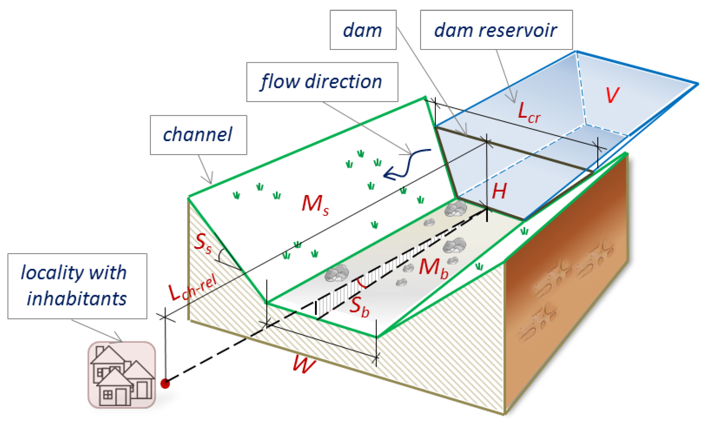
To describe the shape and dimensions of the dam and reservoir, it was assumed that the dam cross section can be described as an isosceles trapezoid with height equal to the dam height, width of the upper base equal to the length of the dam crest, and side slopes equal to the abutment slopes of the dam [63]. The width of the bottom base of the dam is assumed to be the same as the average bottom width of the valley downstream of the dam. The reservoir created by the dam has a planar bed and a trapezoidal cross section that is equal to the one of the dam. Representing the worst-case scenario, the water depth in the reservoir is equal to the dam height. Values of the parameters for dimensions and shape of the dam reservoir are constant over the length of the domain, i.e., prismatic shape of the reservoir.

With these assumptions, three input parameters are required to define the shape and dimensions of the dam and its reservoir; they are the dam height, H (m), the length of the dam crest, ${\mathrm{L}}_{\mathrm{cr}}$ (m), and the volume of the reservoir, V (m³). Units and definitions of these parameters are given in Table 1 for visualization purposes these parameters are shown in Figure 2. Other characteristics of the dam and reservoir (e.g., the reservoir cross section, A (m²), reservoir length, ${\mathrm{L}}_{\mathrm{re}}$ (m), etc.) can be estimated using the abovementioned inputs.

To describe the shape and dimensions of the downstream area (i.e., valley), a simplified geometry was proposed [64]. To define what kind of simplified geometry can rather accurately reflect the population of valleys downstream of the representative hydropower dams in Switzerland, a classification of valleys downstream of the 14 Swiss concrete arch hydropower dams taller than 100 m (Table S1) was performed. It should be noted that classification of natural valleys can be controversial because each natural valley is unique. Therefore, the classification performed in this study considers only major features of the valleys.

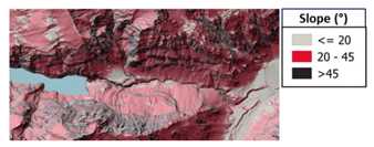
For the purpose of classification, slope maps were generated for the area downstream of each of these 14 dams. Slope data were extracted from the Swiss high-resolution digital elevation model, swissALTI3D [65], and then all slope values were partitioned into three groups: “flat”—flatter than 20°; “moderately steep”—between 20° and 45°; and “steep”—steeper than 45°. Based on the obtained data and on the work about categorization of natural valleys conducted by Rosgen [66] and Rosgen et al. [67], three classes of valleys were defined (

Table 2. Classification of the valleys downstream of 14 concrete arch hydropower dams in Switzerland.

Valley Type Based on Rosgen [66] & Rosgen, Rosgen, Collins, Nankervis and Wright [67]		Dam-downstream Valleys in Switzerland Simplified Geometry
Class 1: Channel with a triangular cross section
Moderately steep, gentle-sloping side-slopes (often in colluvial valleys)	Steep, confined, V-notched canyons, rejuvenated side-slopes	Zevreila dam	Channel with a triangular cross section
Class 2: Channel with a trapezoidal cross section
Moderately steep, U-shaped glacial-through valleys	Santa Maria dam	Moiry dam	Channel with a trapezoidal cross section
Class 3: Other topographies
Joint-, bedrock-controlled valleys	Gigerwald dam		Channel with a rectangular cross section

).

Among the defined classes, the V-shaped valleys (Class 1) have a narrow bottom with moderately steep side slopes (i.e., 20°–63°). This class corresponds to valleys with steep, moderately steep, or gentle-sloping sides as defined in Rosgen [66] and Rosgen, Rosgen, Collins, Nankervis and Wright [67] (Table 2). A good approximation for valleys of this class can be a channel with a triangular cross section. The U-shaped valleys (Class 2) have a distinct valley bottom and moderately steep slopes forming the valley walls that start from the edges of the valley bed. Therefore, this class is reflected in the categorization by Rosgen as moderately steep, U-shaped glacial-through valleys. Valleys of Class 2 can be represented by a channel with a trapezoidal cross section. Finally, valleys of Class 3 are like bedrock valleys with steep side slopes; they also have a pronounced bottom area as in Class 2, but their sides are steeper, i.e., almost vertical (≥75°). Therefore, this class is represented by rectangular-shape cross sections.

Based on the simplified geometries defined for the three classes, a generic model of the downstream valley reflecting all three classes could be defined as a channel with the trapezoidal cross section with two extreme cases, namely the rectangular and triangular cross sections. Therefore, the shape and dimensions of the channel with the simplified geometry can be characterized using four parameters: the channel length relative to the height of the dam, ${\mathrm{L}}_{\mathrm{ch}-\mathrm{rel}}$ (m/m), the channel width, W (m) (uniform for the entire length of the channel), the slope of the channel bed, ${\mathrm{S}}_{\mathrm{b}}$ (m/m) (the same along the entire channel length), and the slope of the channel side slopes, ${\mathrm{S}}_{\mathrm{s}}$ (°) (the same on the right and on the left side of the channel and constant along the entire channel length).

Finally, to account for the surface resistance to the flow, the surface of the channel is described by the roughness coefficients, where roughness values for channel bed, ${\mathrm{M}}_{\mathrm{b}}$ (s/m^1/3), and channel side slopes, ${\mathrm{M}}_{\mathrm{s}}$ (s/m^1/3), are distinguished. The latter are assumed to be the same on both side slopes.

3.1.2. Required Model Response

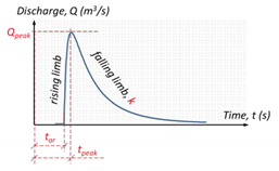
As output, the model provides time series of the flow quantities downstream of the dam. The flow quantities, namely the outflow hydrograph, maximum water depth, ${\mathrm{h}}_{\max }$, and maximum water velocity, ${\mathrm{v}}_{\max }$, at the last downstream cross section of the channel are the outputs of interest. Although the parameters ${\mathrm{h}}_{\max }$ and ${\mathrm{v}}_{\max }$ are self-explanatory, the shape of the hydrograph generally can be described using the following features. Taking into account that the downstream area is initially dry (i.e., no base flow) and that the flood was caused by a water release from the dam reservoir and not by a rainfall event (i.e., the basin lag time is substituted by the time to the peak discharge), the peak discharge, the time to the peak discharge, the time of the flood arrival, and the recession constant can sufficiently describe the shape of the hydrograph (

Table 3. Definition of hydrograph features.

Feature	Definition	Visualization
Peak discharge, $Q_{peak}$, (m3/s)	Maximum outflow reached during the flood event
Time-to-peak discharge, $t_{peak}$, (s)	Time interval between the start of the computational time and the peak discharge
Time-to-flood arrival, $t_{ar}$, (s)	Time interval between the start of the computational time and the time of the first non-zero discharge value. Knowing $t_{peak}$, $t_{ar}$, and $Q_{peak}$ the rising limb of the hydrograph can be built, i.e., the curve reflecting the increase of the discharge.
Recession constant, $k$, (m3/s2)	The recession limb begins at time to peak and continues while the value of discharge decreases. This limb is characterized by a recession constant, k, of the line between the peak discharge and a discharge at time t after the peak discharge.

) [68].

Although values for all the hydrograph features can be set based on their definition, the recession constant, $\mathrm{k}$ (m³/s²), can be calculated as [69]:

$$k=\left(ln\left(Q_{peak}\right)-ln(Q_t)\right)/\Delta t$$

(9)

where, $Q_t$ (m³/s) is the discharge at time t, which corresponds to the total run time and $\Delta \mathrm{t}$ (s) is the time between $t_{peak}$ and $t$. In this study, the total run time was set to a conservative value of 9000 s, allowing for the computation of the model output and also for extreme-case scenarios.

3.2. Step B. Modeling the Sources of Uncertainties

For the majority of the model input parameters, the initial dataset contained 14 data points. Therefore, the maximum entropy principle was used to define distributions for this model (Section 2.3.2). According to the maximum entropy principle, the least biased Probability Density Function (PDF) $f_X\left(x\right):\Omega ⟼D_{X}c{R}_{int}$ for representing information about a continuous variable X is the one that maximizes its entropy $H\left[f_X\right]$ (as defined in Equation (10)), as well as certain constraints based on the available information, e.g., bounds, moments, etc.

$$H\left[f_X\right]\stackrel{\mathrm{def}}{=}{{\displaystyle \int }}_{D_X}-f_X\left(x\right)ln{f}_X\left(x\right)dx=E\left[-ln{f}_X\left(X\right)\right]$$

(10)

In this study, entropy was tested between uniform and beta distributions (

Table 4. Probability distributions used to build marginal distributions for the model input parameters.

Distribution	Density Function	Parameters	Entropy
Beta $B\left(\alpha ,\beta \right)$	$f\left(x\right)=\frac{x^{\alpha -1}{\left(1-x\right)}^{\beta -1}}{B\left(\alpha ,\beta \right)}$, for x defined on the support [0,1] or (0,1)	Where $B\left(\alpha ,\beta \right)$ is the Beta function, $\alpha =\mu \left(\left(\mu \left(1-\mu \right)/\sigma \right)-1\right)$ is a first shape parameter and $\beta =\left(\mu \left(1-\mu \right)/\sigma \right)\left(1-\mu \right)$ is a second shape parameter. A Beta distribution is an alternative for bounded parameters with non-uniform distributions.	$H\left(x\right)=ln\left[B\left(\alpha ,\beta \right)\right]-\left(\alpha -1\right)\left[\psi \left(\alpha \right)-\psi \left(\alpha +\beta \right)\right]-\left(\beta -1\right)\left[\psi \left(\beta \right)-\psi \left(\alpha +\beta \right)\right]$, where $\psi \left(c\right)$ is the first derivative of Euler’s gamma
	for y with a support [$a_B$, $b_B$] or ($a_B$, $b_B$): $y=x\left(b_B-a_B\right)+a_B$ Therefore, $f\left(y;\alpha ,\beta ,a_B,b_B\right)=\frac{{\left(y-a_B\right)}^{\alpha -1}{\left(b_B-y\right)}^{\beta -1}}{{\left(b_B-a_B\right)}^{\alpha +\beta -1}B\left(\alpha ,\beta \right)}$
Uniform $U\left(a,b\right)$	$f\left(x\right)=\frac{1}{b-a}$ $forx\in \left[a,b\right]$ $\left(otherwisef\left(x\right)=0\right)$	Where $a=\mu -\sqrt{3}·\sigma$ is a lower boundary and $b=\mu +\sqrt{3}·\sigma$ is an upper boundary. A Uniform distribution is applied when little is known about the parameter (e.g., distance, loads).	$H\left(x\right)=ln\left(b-a\right)$

), which are normally used when little knowledge about the parameter is available (e.g., little confidence in the computed mean or median of the data). Furthermore, both distributions are bounded, allowing for setting the limits based on the range of values for the population of dams. For each of the two distribution types, the equations for entropy are given in Table 4. To identify the parameters of the distributions (Table 4), the maximum likelihood principle was used as explained in Section 2.3.2.

To model the distributions of physical characteristics of the dam and reservoir, information about the population of dams in Switzerland was gathered. In order to build probability distributions for H (m), $L_{cr}$ (m), and V (m³), data about 14 concrete arch dams taller than 100 m (Table S1) were used (Swiss Committee On Dams [5]). By testing entropy for two probability distribution types (Section 2.3.2), it was found that the length of the dam crest was uniformly distributed [Figure 3a]. In the case of dam height, it is known that lower values of the distribution range will have higher probabilities, i.e., the frequency of having a dam with a lower height is higher. Therefore, a beta distribution was used to describe the dam height [Table 6, Figure 3b], where $a_B$ and $b_B$ are the bounds of the height range for the Swiss arch concrete dams taller than 100 m. Because the reservoir volume is strongly correlated with the dam height, it was assumed that V was also following a beta distribution [Table 6, Figure 3c].

To build probability distributions for the parameters of the channel (i.e., ${\mathrm{L}}_{\mathrm{ch}-\mathrm{rel}}$, W, ${\mathrm{S}}_{\mathrm{s}}$, ${\mathrm{S}}_{\mathrm{b}}$), information was extracted from the topographic maps and digital elevation maps [65] of the areas downstream of the 14 arch dams considered (Table S1).

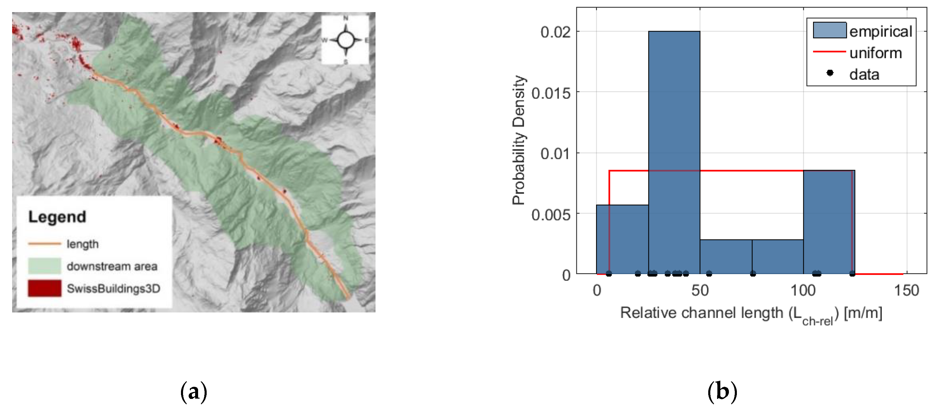
The channel length was estimated as the distance between the dam and the nearest locality with at least 500 inhabitants situated downstream of the dam [Figure 4a]. The distance corresponds to the flow path, i.e., considering all bends in the reach. For each dam, the locality situated either along the channel or at the end of the channel was chosen (Table S1). For example, in the Mauvoisin dam case, the channel length is measured between the dam and the Bagnes town, with the population of 8057 people as in 2016 [70]. Based on these measurements, the channel length relative to the height of the dam, ${\mathrm{L}}_{\mathrm{ch}-\mathrm{rel}}$, was described with a uniform distribution [Table 6, Figure 4b].

The channel slope ${\mathrm{S}}_{\mathrm{b}}$ was defined by the difference in elevation between the dam and the locality and the absolute value of the channel length (i.e., not normalized by the dam height). Based on the collected data, ${\mathrm{S}}_{\mathrm{b}}$ was found to follow a beta distribution truncated over the boundary corresponding to the smallest and the largest existing values (Table 6).

According to the definition given in Section 3.1.1, the channel bed is defined using the swissALTI3D slope map [65]. Then, multiple lines were drawn across the bed area perpendicular to the channel axis, where each line represented the width of the channel bed in a specific location [as shown, for example, in Figure 5a]. For each channel the average value of W was taken into account to build a generic distribution representing all channels. The channel bed width was uniformly distributed [Table 6, Figure 5b].

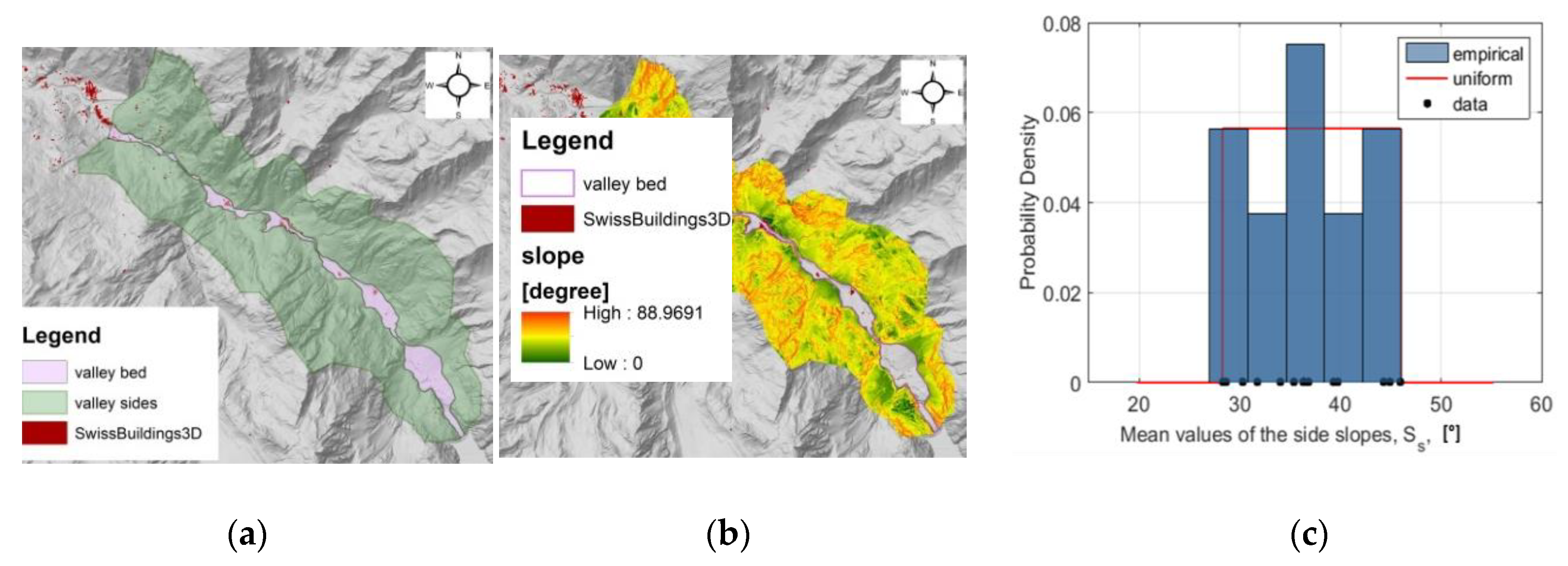
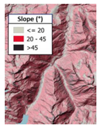
To define the channel side slope $S_s$ for each individual valley the following steps were performed, as shown for the case of the Mauvoisin dam in Figure 6a–c. First, the polygon of the valley embankments was drawn [Figure 6a, green polygon]. This polygon indicated the area that is lying below the mountain ridge forming the sides of the valley, but that is not included in the polygon of the valley bed [Figure 6a, rose polygon). In the next step, the slope value at each point falling within the defined polygon was extracted from the swissALTI3D slope map [Figure 6b]. Then, the mean of the slope was computed assuming that $S_s$ for each valley was normally distributed. Figure 6c presents an empirical histogram of all 14 calculated $S_s$ values showing that $S_s$ is uniformly distributed (Table 6).

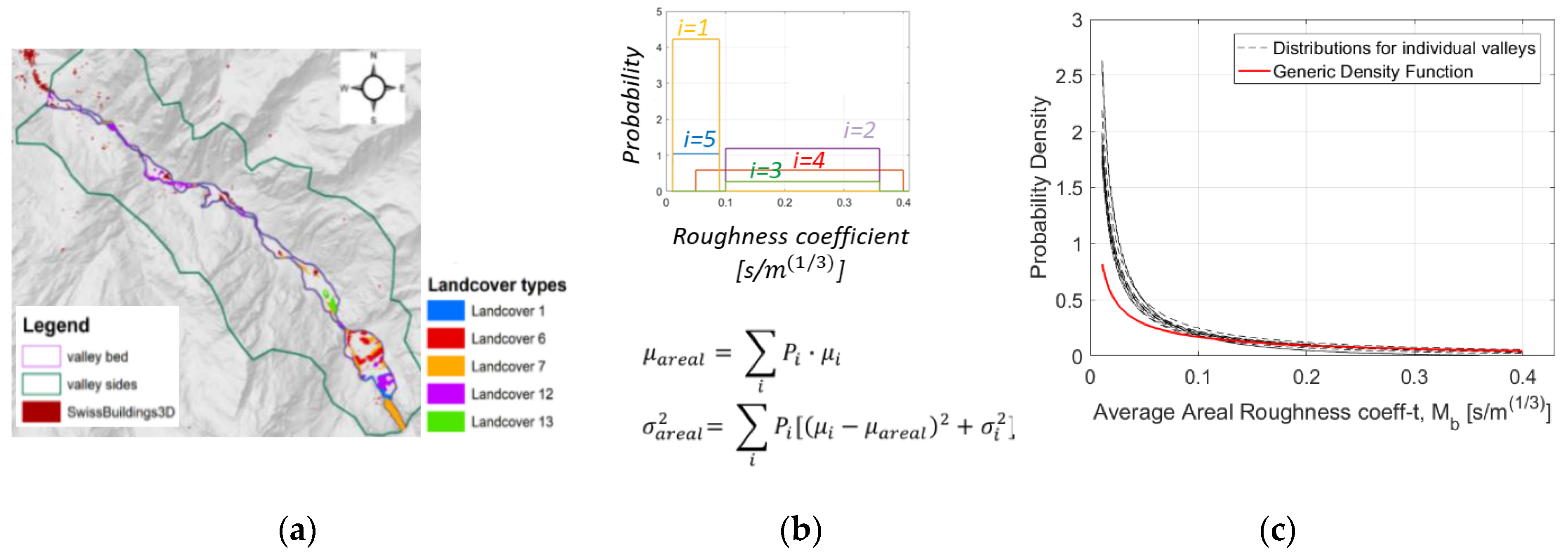
The downstream environment is characterized by the roughness coefficients $M_b$ and $M_s$. Figure 7a–c shows three steps performed to build a probability distribution for $M_b$ based on the data about the 14 valleys. The process of building a probability distribution for $M_s$ is analogous.

In the first step [Figure 7a], the types of land cover in the areas downstream of the dam were collected using data from the Swiss topographic landscape model, swissTLM3D [71]. The swissTLM3D differentiates between six types of land cover (

Table 5. Roughness coefficients for different types of land cover.

Landcover Type (SwissTLM3D)	Number	Name According to US National Land Cover Dataset (NLCD)	Manning’s Coefficients (s/m1/3)
Rock	1	barren land	0.011–0.09
Shrubbery forest	6	shrub/scrub	0.05–0.4
Soil, earth	7	barren land	0.011–0.09
Wetlands	11	woody/emergent herbaceous wetlands	0.086–0.14/0.045–0.3
Forest	12	deciduous forest/evergreen forest	0.1–0.36/0.1–0.32
Forest (open)	13	deciduous forest/evergreen forest	0.1–0.36/0.1–0.32

). In this study, water bodies were excluded as a land cover type, because the downstream area of the dam was treated as a dry domain due to much smaller size of any water body in comparison with the dam reservoir.

Manning’s roughness coefficients for different land cover types were defined using information available in the literature. Because many studies [72,73] used the NLCD classification (i.e., National Land Cover Dataset by the US Geologic Survey, [74]), land cover types in the SwissALTI3D classification were allocated to the types of the NLCD classification using the available description (Table 5).

In the second step [Figure 7b], the roughness of each land cover type was described by the average areal roughness with mean, ${\mu }_i$, and variance, ${\sigma }_i^2$, calculated by assuming that the roughness coefficient within each land cover type is distributed uniformly. Furthermore, areal probability, $P_i$, was assigned to each land cover type by defining the fraction of the area occupied by the land cover type in the total area of the downstream valley bed. Then, using the equations given in Figure 7b, the mean, ${\mu }_{areal}$, and the variance, ${\sigma }_{areal}^2$, of the average areal roughness for the entire area of the downstream valley bed were defined. Finally, using the mean ${\mu }_{areal}$ and variance ${\sigma }_{areal}^2$ calculated with the method of moments, the maximum entropy was used to calculate the parameters of a beta probability distribution, which yielded a better fit to the $M_b$ data.

Probability distributions of the average areal roughness, $M_b$, for each valley are displayed as dashed lines in Figure 7c. To construct the distribution of the roughness reflecting the population of all considered valleys, roughness distributions of all distinct land cover types in different valleys were treated together and their areal probabilities were normalized by the total number of considered valleys. This resulted in a beta distribution shown as a red solid line in Figure 7c. The information about chosen marginal distributions, their hyper parameters, truncation range, and moments are summarized for all input parameters in

Table 6. Information about the marginal distributions specified for the input of the metamodel.

Para-Meter	Unit	Distribution	Hyper Parameters	Truncation	Mean and Variance
H	(m)	$H~Beta\left(\alpha ,\beta ,a_B,b_B\right)$	$\alpha =1.28,\beta =2.98,$ $a=100,b=250$	-	159.9, 26.6
V	(m3)	$V~Beta\left(\alpha ,\beta ,a_B,b_B\right)$	$\alpha =1.28,\beta =2.98,$ $a=9200,b=2.1E5$	-	69,890, 40,460
$L_{cr}$	(m)	$L_{cr}~U\left(a,b\right)$	$\mathrm{a}=256,\mathrm{b}=610$	-	433, 102.19
$L_{ch-rel}$	(m/m)	$L_{ch-rel}~U\left(a,b\right)$	$\mathrm{a}=5.9,\mathrm{b}=123.6$	-	64.75, 33.98
$W$	(m)	$W~U\left(a,b\right)$	$\mathrm{a}=1.0,\mathrm{b}=163.66$	-	82.33, 46.96
$S_s$	(°)	$S_s~U\left(a,b\right)$	$\mathrm{a}=28.28,\mathrm{b}=45.98$	-	37.13, 5.11
$S_b$	(m/m)	$S_b~Beta\left(\alpha ,\beta \right)$	$\alpha =3.22,\beta =32.48$	[0.03, 0.23]	0.090, 0.047
$M_b$	(s/m1/3)	$M_b~Beta\left(\alpha ,\beta \right)$	$\alpha =0.33,\beta =2.07$	[0.01, 0.4]	0.14, 0.19
$M_s$	(s/m1/3)	$M_s~Beta\left(\alpha ,\beta \right)$	$\alpha =0.40,\beta =1.88$	[0.01, 0.4]	0.17, 0.12

.

Finally, all input parameters of the model were checked for possible dependence. The results showed strong positive, as well as negative, correlation between some of the inputs. For example, both the correlation between reservoir volume and dam height and the correlation between the crest length and the reservoir volume had a value of 0.57. These results can be supported by findings of other research conducted in the past; for example, the first example of correlation is reflected in the GRanD database guidelines for estimating missing reservoir volumes based on the reservoir area and dam height [75].

A negative correlation was found between the dam height and the relative length of the channel (${\rho }_{H,L_{ch-rel}}=-0.51$), and between the slope of the channel bed and the roughness coefficient of the channel sides (${\rho }_{S_b,M_s}=-0.52$). The later, for example, can demonstrate that it is harder for vegetation such as forest trees to grow on very steep slopes. Correlation coefficients for other combinations are given in

Table 7. Spearman rank correlation coefficients calculated among model input parameters.

Parameter	H	V	${\mathit{L}}_{\mathit{c}\mathit{r}}$	${\mathit{L}}_{\mathit{c}\mathit{h}-\mathit{r}\mathit{e}\mathit{l}}$	W	${\mathit{S}}_{\mathit{s}}$	${\mathit{S}}_{\mathit{b}}$	${\mathit{M}}_{\mathit{b}}$	${\mathit{M}}_{\mathit{s}}$
H	1	0.574	0.218	−0.512	0.082	0.213	−0.020	−0.007	0.125
V		1	0.574	−0.253	0.298	0.112	−0.156	0.046	−0.108
${\mathit{L}}_{\mathit{c}\mathit{r}}$			1	−0.336	0.280	−0.138	0.143	0.196	−0.380
${\mathit{L}}_{\mathit{c}\mathit{h}-\mathit{r}\mathit{e}\mathit{l}}$				1	0.417	−0.341	−0.385	0.354	0.165
W					1	−0.179	−0.347	0.378	0.223
${\mathit{S}}_{\mathit{s}}$						1	0.196	−0.442	−0.380
${\mathit{S}}_{\mathit{b}}$							1	−0.073	−0.521
${\mathit{M}}_{\mathit{b}}$								1	0.292
${\mathit{M}}_{\mathit{s}}$									1

.

3.3. Step C. Uncertainty Propagation

The generic PCE metamodel for each of the defined model outputs was calculated using the experimental design with a sample size of 2000. The correlation between the model inputs was not considered for building the metamodel to achieve better metamodeling performance [76]. Afterwards, the constructed PCEs were evaluated on the new sample set of size 1,000,000 using coefficients calculated in the previous step. Prior to the forward propagation of the input uncertainties, the information about correlation between model inputs, i.e., Gaussian Copula with calculated Spearman rank correlation coefficients, was added to the information about marginal distributions and their bounds. In this way, the final PDF distributions reflecting uncertainty of the model outputs were built, including the information about the dependency between input parameters.

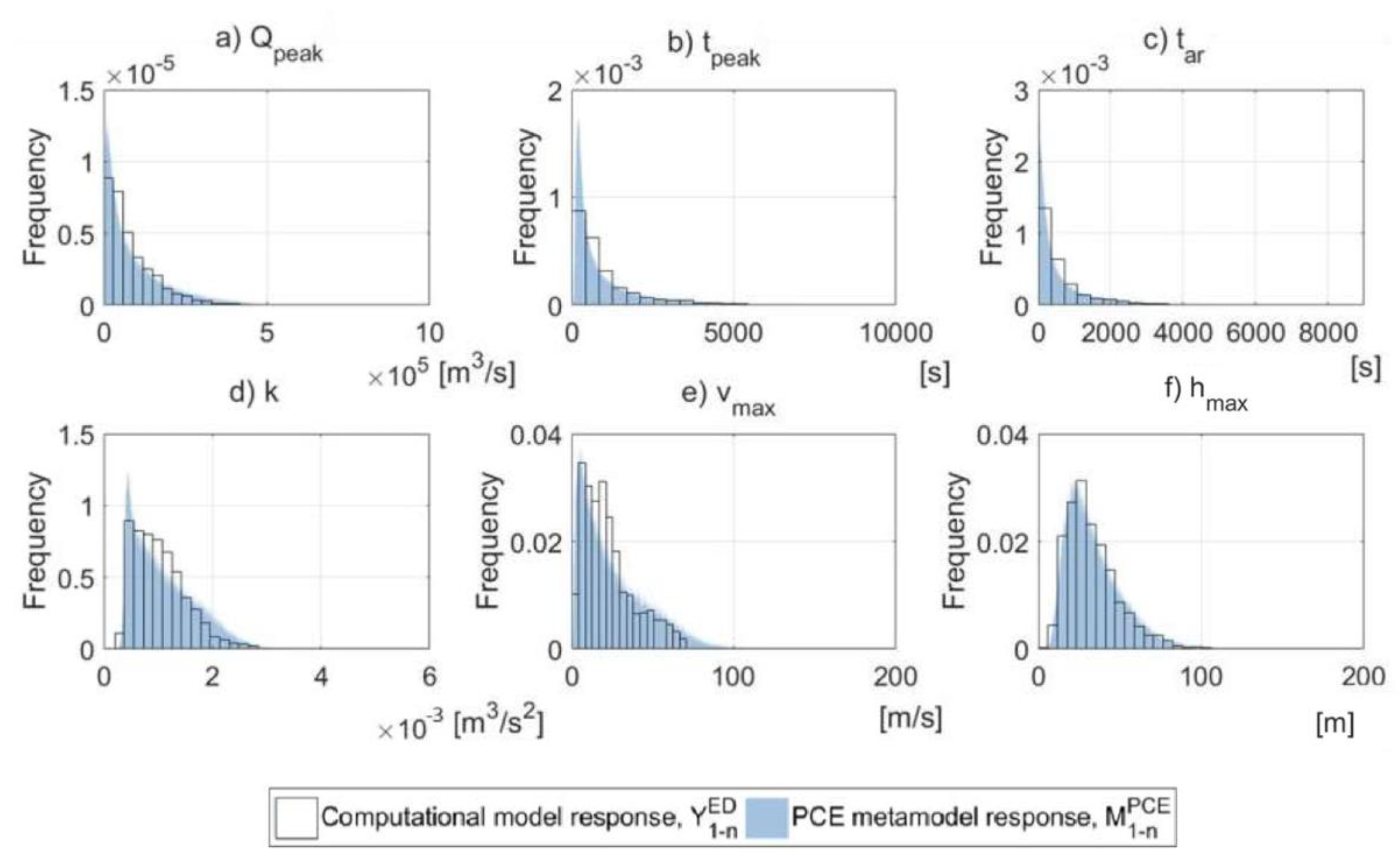
In Figure 8a–f, the histograms of the computational model responses, $Y_{1-6}^{ED}$, and the histograms of the PCE metamodel response, $M_{1-6}^{PCE}$, are shown. The latter together with the calculated moments of the metamodel response reflect the variability of the modeled parameters. In particular, the mean value of the peak discharge is 0.99 × 10⁵ m³/s and the arrival of this peak outflow corresponds to 1067 s (17.78 min), whereas arrival of the flood itself corresponds to 756 s (12.60 min). However, the range of possible values of the corresponding parameters is large and the values of the peak outflow and the time to the peak outflow can grow up to 7 × 10⁵ m³/s and 9000 s (150 min), respectively. The results for the recession constant describing the hydrograph indicate that the descending limb is a flat curve (i.e., the mean value of the recession constant k is 0.98 × 10⁻³ m³/s²), demonstrating that the water tends to remain at the location, i.e., the decrease in water depth is slow. The mean value of the maximal flow velocity is 26.19 m/s and the mean value of maximum water depth is 34.42 m, which are rather high considering that they indicate the most severe moment when the flood wave arrives.

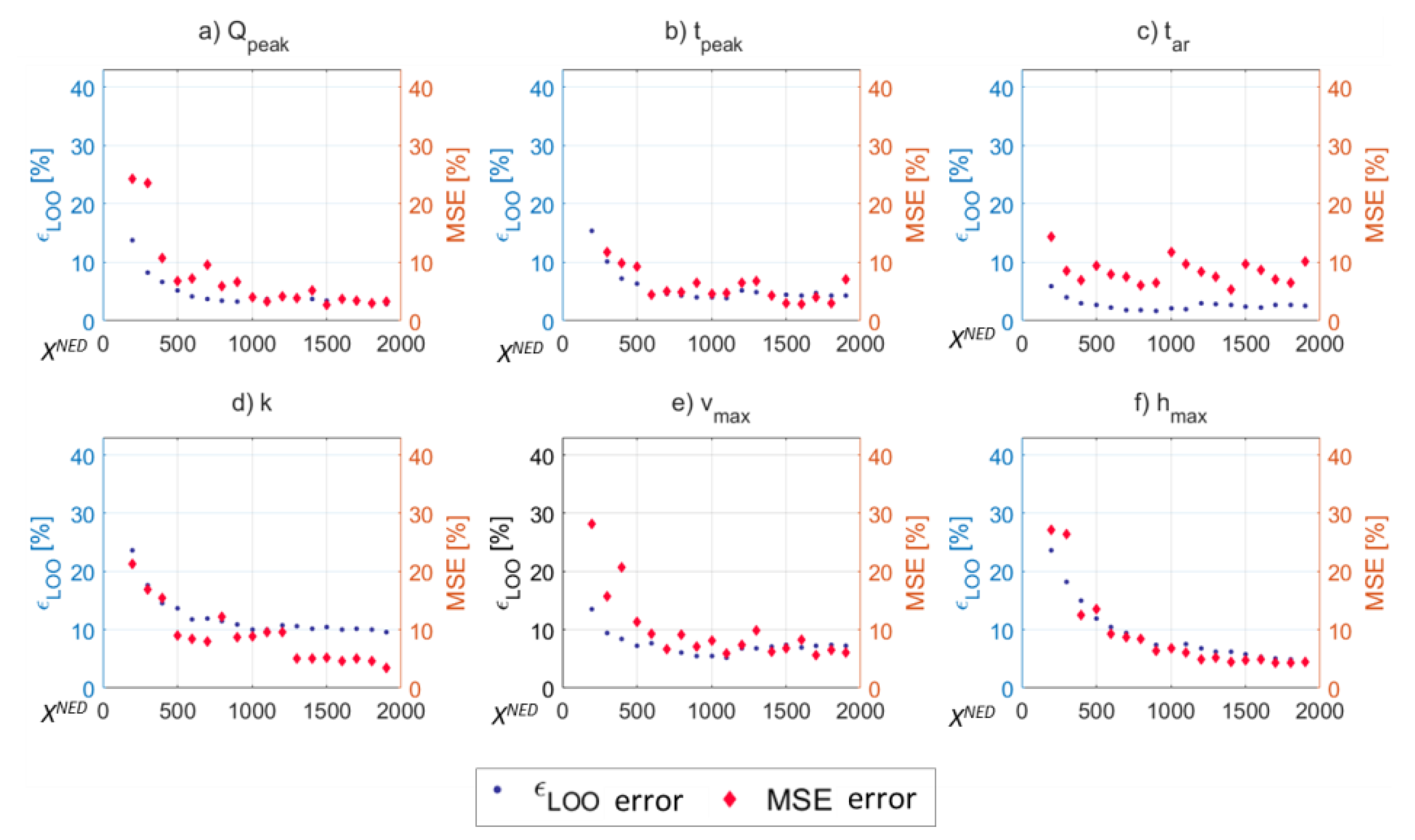
Quantitative validation of the calculated PCEs was done by estimating the cross-validation error (${ϵ}_{LOO}$). Results are given in Figure 9 and Table S2 for different experimental designs. The PCE degree shown in the appendix is the PCE degree with the lowest ${ϵ}_{LOO}$ in the array of the given degrees (i.e., 1–15) [54]. The results showed that with the increasing ED the value of ${ϵ}_{LOO}$ decreases, and the degree of the calculated PCE changes as well. The residual ${ϵ}_{LOO}$ for some of the model outputs is about 10% (e.g., $k,v_{max}$).

Because of the relatively high residual ${ϵ}_{LOO}$, in addition to the built-in error estimation, the mean squared error (MSE) was used as another error metric for the convergence of the mean values of the model outputs. For this analysis, the ED was divided into two samples, where one was used for construction of the PCE, $X^{NED}$, and another as a validation sample, $X^{VAL}$. While $X^{VAL}$ was represented by the same sample set of 100 points, $X^{NED}$ was increased stepwise from 200 to 1900 sample points (see Figure 9). Then, the validation error evolution using the prediction of PCE, $Y^{NED}$, and the true output of the computational model, $Y^{VAL}$, was calculated as:

$$MSE=\frac{\frac{{{\displaystyle \sum }}_{i=1}^n{\left(Y_i^{NED}-Y_i^{VAL}\right)}^2}{n}}{\frac{{{\displaystyle \sum }}_{i=1}^n{\left(Y_i^{VAL}-{\overline{Y}}^{VAL}\right)}^2}{n}},\mathrm{where} {\overline{Y}}^{VAL}=\frac{{{\displaystyle \sum }}_{i=1}^n{Y}_i^{VAL}}{n}$$

(11)

The calculated MSE (Figure 9 and Table S2) decreases for all the model outputs with the larger size of the ED, $Y^{NED}$. For some of the parameters the decrease of the MSE value is rather constant and well-pronounced (e.g., $Q_{peak},k,h_{max}$); for some others the MSE value decreased to 10% rather quickly and then stayed rather constant at the same level with the enlarging ED (e.g., $t_{peak},t_{ar}$). Similar to ${ϵ}_{LOO}$, the residual MSE for some parameters is about 10%. The overall tendency of MSE to decrease with an increasing ED is an indicator that the applied computational model is complex. In addition, the repeatability error calculated for each of the model outputs is close to 0.1% or substantially lower than this value (Protocol S1), which is another indicator of the model complexity.

The validation results with the residual error (both ${ϵ}_{LOO}$ and MSE) of 10% might compromise the advantages of using PCE as a tool for UQ. However, studies conducted in the past were able to prove that if the metamodel is used for the estimation of the statistical properties of the model output (e.g., mean, variance) and also for calculation of sensitivity indices (Section 3.4), then it is rather accurate even with a residual error of about 10% [25]. Another factor that can potentially contribute to relatively high validation error (both ${ϵ}_{LOO}$ and MSE) is the nature of the model outputs defined in this study. Most of them represent maxima parameters (i.e., $Q_{peak},v_{max},h_{max}$) and the peaks are intrinsically harder to metamodel.

Finally, other types of surrogate modeling techniques, such as low-rank approximation (LRA) [16] and Gaussian process modeling (i.e., kriging [77]), were tested. Although LRA is particularly promising for high-dimensional problems (i.e., the number of unknown coefficients in LRA grows only linearly with respect to the input dimension [16]) and kriging has a different approach to approximate Y (i.e., it focuses on the local alterations of Y, whereas PCE approximates the global behavior of Y [78]), both of these metamodeling approaches did not reveal a better fit to the computational model.

3.4. Step D. Global Sensitivity Analysis

In general, the PCE approach reduces the cost of GSA by calculating the Sobol’ indices directly from the PCE coefficients, ${\mathrm{y}}_{\mathsf{\alpha }}$, without the need for additional sampling (see Section 2.5). However, in real applications different issues can arise. An example can be cases of high-dimensional models, such as the one applied in this study (i.e., the model has nine inputs). For these models, UQ sampling of the size ${10}^2$ to ${10}^3$ still allows to reach a good agreement with the computational model, but for the calculation of the Sobol’ indices a sample size ${10}^4$ to ${10}^5$ is normally required. In other words, if the computational cost for building the metamodel itself does not depend on the dimensionality of the model, the computational cost for the GSA increases with larger model dimensions. However, for the particular case of the “structural” GSA (Section 2.5), sampling of the size ${10}^2$ to ${10}^3$ could be adopted, and the metamodel built in Section 3.3 on the ED of 2000 points was used also for GSA.

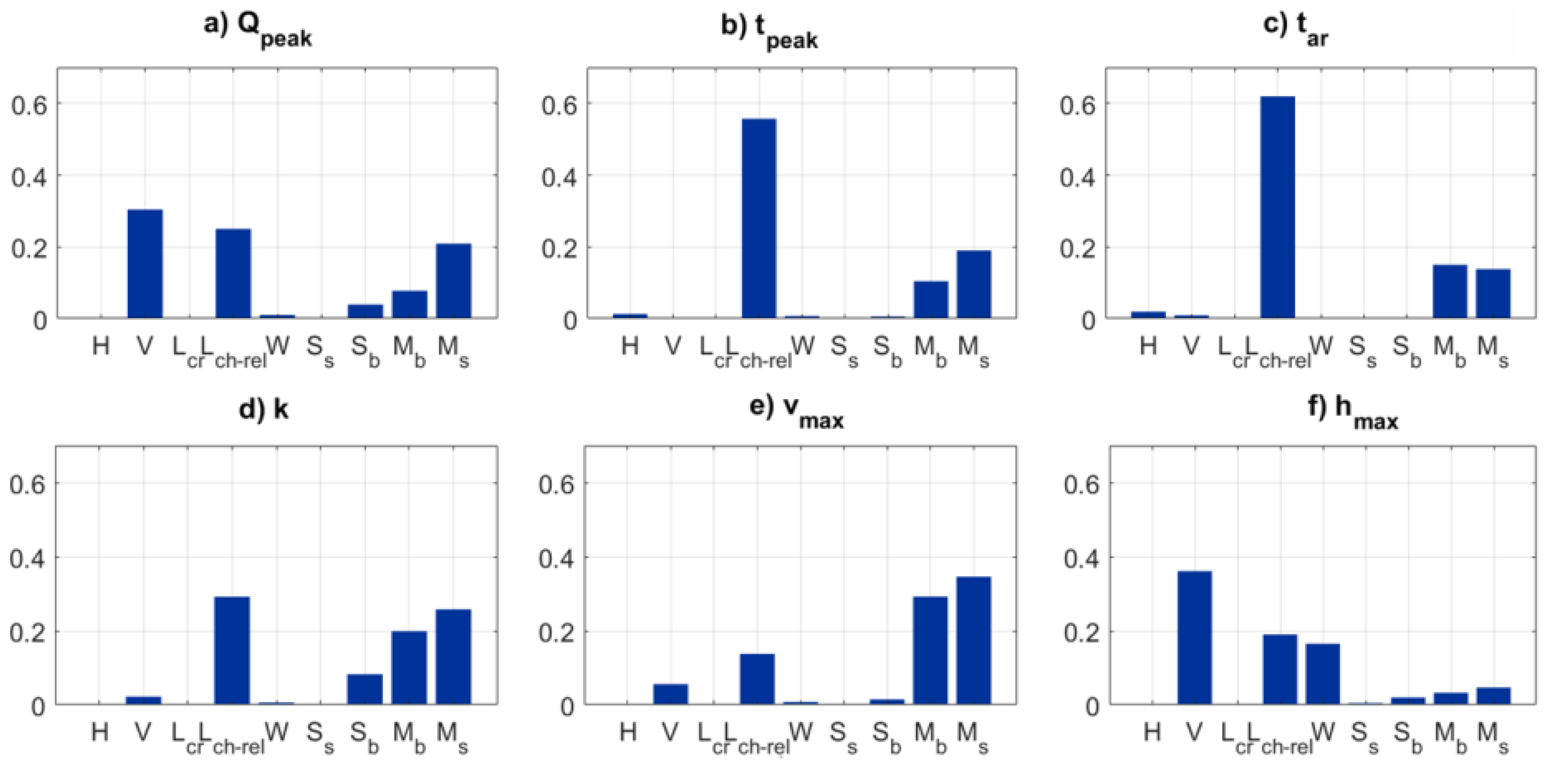
The calculated first-order Sobol’ indices (Figure 10a–f) indicate that among the parameters characterizing the dam and its reservoir (i.e., $H,V,L_{cr}$), the reservoir volume, V, is the most important for the parameters $Q_{peak}$ and $h_{max}$. In other words, the volume of the water released from the dam reservoir influences amounts of water reachable downstream, which are expressed as outflow or water depth. Meanwhile, dam height, H, and crest length, $L_{cr}$, did not influence any of the flow quantities estimated at the end of the channel.

Among the parameters of the channel, the relative length, $L_{ch-rel}$, strongly affected all model outputs. In other words, by moving further downstream from the dam, not only did the maximum reachable flow quantities ($Q_{peak},v_{max},h_{max}$) changed, but the shape of the hydrograph ($t_{peak},t_{ar}$, k) was altered. The width of the channel bed, W, is relatively important only for $h_{max}$; the water has literally more space to spread. Lastly, the slope of the channel bed, $S_b$, and sides, $S_s$, did not show influence over any of the model outputs.

Finally, the roughness coefficients had influence on the characteristics of the hydrograph ($Q_{peak},t_{peak},t_{ar},k$) and the maximum velocity reached downstream, $v_{max}$. Roughness corresponds to flow resistance, e.g., the velocity decreases and it takes more time for the discharge to arrive and to reach its peak. The influence of $M_s$ on the output parameters is slightly higher than the influence of $M_b$, which may be simply related to the fact that the channel sides cover a substantially larger surface area than the channel bed.

The calculated sensitivity indices identified the model input parameters that are influential for the model describing large hydropower dams in Switzerland. When variability of the output has to be limited, further investigation of the influential inputs needs to be done to decrease their uncertainty. For example, in the context of the dam risk assessment, to make a better prediction of the potential loss of life due to the impact of the dam-break flood wave, uncertainty of the value of the outflow, flow velocity, and maximum water depth at the location of the city needs to be decreased. According to the sensitivity results, to achieve that, the volume of the dam reservoir needs to be measured or monitored accurately. Furthermore, the roughness, especially of the channel sides, may be defined more specifically. For example, the average areal roughness used in this study can be further investigated to reflect different roughness on various parts of the valley.

4. Conclusions

The current study demonstrated the application of metamodeling for quantitative assessment of uncertainties for the complete and instantaneous break of a hypothetical concrete dam located in Switzerland. A 1D model based on the Shallow Water Equations was used for numerical simulation of the flood wave propagation. The model configuration included nine input parameters characterizing the dam, its reservoir and the downstream area and six model outputs defined as the flow quantities reached downstream of the failed dam. This computational model was approximated with a metamodel.

A polynomial chaos expansion (PCE) was able to reproduce the computational model with good agreement using 2000 runs of the original model. This offers the opportunity to reduce computational efforts compared, for example, to Monte Carlo sampling, which was applied in Froehlich [79] and required 100,000 trials to estimate confidence limits of dam-breach flood calculations. Furthermore, the quantitative assessment of uncertainties, which was enabled by using the metamodel, is beneficial for further phases of modeling the dam-break event. For example, it allows for the description of the flow quantities reached downstream in form of probability distributions, which then can be used as uncertain inputs to the model for the loss of life estimation in the downstream area.

The applied metamodeling approach also allowed sensitivity analysis by calculating the first-order PCE-based Sobol’ indices. These indices helped to understand how the variability of each model input affected variability of the model output and to identify important sources of discrepancy within the model. Particularly, the reservoir volume, length of the channel, and surface roughness in the downstream area were important parameters that drove the output of the model as reflected by the higher values of the Sobol’ indices. The dam dimensions, as well as slopes of the channel sides and bed, did not significantly influence the flow quantities at the end of the channel, i.e., at the locality of population at risk.

Finally, the constructed metamodel can support decision-making processes in risk management for large concrete arch hydropower dams in mountain regions of Switzerland. By setting certain parameters to deterministic values and by further specifying the distribution of the remainder of the parameters based on the specific location, this generic metamodel is converted into a preliminary model of the failure of a dam to be built in the future. Then, the flow quantities that can be reached downstream can be quickly approximated without running any computationally expensive model, what is useful for risk assessment and decision support. These findings eventually provide important inputs for decision makers when formulating energy policy strategies.

As an outlook of the current research, if it is decided to switch to 2D flood propagation models to account for non-prismatic channels and valleys with more complex topographies, robustness of PCE for quantitative assessment of uncertainties has to be investigated. Furthermore, correlation among input parameters and their influence on variability of the model output can be further addressed in sensitivity analysis. For this purpose, alternative techniques, e.g., Borgonovo indices [80] or copula-based approaches [81,82], can be applied. However, their application should be done with caution since it strongly depends on the question asked before doing the analysis. Finally, the step of life-loss estimation due to a dam-break will be addressed by the authors in the follow-up research.

References

1. Lafitte, R. Classes of risk for dams. Hydropower Dams 1996, 6, 59–66. [Google Scholar]
2. Molinaro, P. Dam break analysis: A state of the art. In Computational Water Resources; Bensar, D., Brebbia, C.A., Ovazar, D., Eds.; CMP: Boston, MA, USA, 1991. [Google Scholar]
3. Betamio de Almeida, A.; Bento Franco, A. Modeling of dam break flows. In Computer Modeling of Free Surface and Pressurized Flows; Chaudhry, M.H., Mays, L.W., Eds.; NATO ASI Series: Heidelberg, Germany, 1993; pp. 343–375. [Google Scholar]
4. ICOLD. Dictionary. International Commission on Large Dams. Available online: http://www.icold-cigb.net/GB/Dictionary/dictionary.asp (accessed on 3 May 2016).
5. SwissCOD. Dams in Switzerland. Available online: http://www.swissdams.ch/index.php/en/swiss-dams/dams-in-switzerland (accessed on 5 May 2018).
6. Zhang, L.; Peng, M.; Chang, D.; Xu, Y. Dam Failure Mechanisms and Risk Assessment; Jon Wiley and Sons, Inc.: New York, NY, USA, 2016. [Google Scholar] [CrossRef]
7. Pearce, F. Dams and Floods; WWF: Gland, Switzerland, 2001. [Google Scholar]
8. Froehlich, D.C. Peak Outflow from Breached Embankment Dam. J. Water Resour. Plan. Manag. 1995, 121. [Google Scholar] [CrossRef]
9. Teng, J.; Jakeman, A.J.; Vaze, J.; Croke, B.F.W.; Dutta, D.; Kim, S. Flood inundation modeling: A review of methods, recent advances and uncertainty analysis. Environ. Model. Softw. 2017, 90, 201–216. [Google Scholar] [CrossRef]
10. Cao, Z.; Pender, G.; Wallis, S.; Carling, P. Computational dam-break hydraulics over erodible sediment bed. J. Hydraul. Eng. 2004, 130, 689–703. [Google Scholar] [CrossRef]
11. Zagonjolli, M. Dam Break Modeling, Risk Assessment and Uncertainty Analysis for Flood Mitigation. Ph.D. Thesis, Delft University of Technology and of the Academic Board of the UNESCO-IHE Institute for Water Education, Delft, The Netherlands, 2007. [Google Scholar]
12. Hartford, D.; Baecher, G. Risk and Uncertainty in Dam Safety; Thomas Telford Publishing: London, UK, 2004. [Google Scholar]
13. Peter, S.J.; Siviglia, A.; Nagel, J.; Marelli, S.; Boes, R.M.; Vetsch, D.; Sudret, B. Development of probabilistic dam breach model using Bayesian inference. Water Resour. Res. 2018, 54, 4376–4400. [Google Scholar] [CrossRef] [Green Version]
14. Romanowicz, R.; Beven, K. Estimation of flood inundation probabilities as conditioned on event inundation maps. Water Resour. Res. 2003, 39, SWC41–SWC412. [Google Scholar] [CrossRef]
15. Bates, P.D.; Horritt, M.S.; Aronica, G.; Beven, K. Bayesian updating of flood inundation likelihoods conditioned on flood extent data. Hydrol. Process. 2004, 18, 3347–3370. [Google Scholar] [CrossRef]
16. Konakli, K.; Mylonas, C.; Marelli, S.; Sudret, B. UQLab User Manual—Canonical Low-Rank Approximations; Report UQLab-V1.1-108; Chair of Risk, Safety & Uncertainty Quantification, ETH Zürich: Zurich, Switzerland, 2018. [Google Scholar]
17. Yazdi, J.; Salehi Neyshabouri, S.A.A. Adaptive surrogate modeling for optimization of flood control detention dams. Environ. Model. Softw. 2014, 61, 106–120. [Google Scholar] [CrossRef]
18. Dwelle, M.C.; Kim, J.; Sargsyan, K.; Ivanov, V.Y. Streamflow, stomata, and soil pits: Sources of inference for complex models with fast, robusr uncertainty quantification. Adv. Water Resour. 2019, 125, 13–31. [Google Scholar] [CrossRef]
19. Ginsbourger, D.; Rosspopoff, B.; Pirot, G.; Durrande, N.; Renard, P. Distance-based kriging relying on proxy simulations for inverse conditioning. Adv. Water Resour. 2013, 52, 275–291. [Google Scholar] [CrossRef] [Green Version]
20. Razavi, S.; Tolson, B.A.; Burn, D.H. Review of surrogate modeling in water resources. Water Resour. Res. 2012, 48. [Google Scholar] [CrossRef]
21. Xiu, D.; Karniadakis, G. The Wiener-Askey polynomial chaos for stochastic equations. SIAM J. Sci. Comput. 2002, 24, 619–644. [Google Scholar] [CrossRef]
22. Schöbi, R.; Sudret, B. Combining Polynomial Chaos Expansions and Kriging; RSUQ-2014-001; Chair of Risk, Safety and Uncertainty Quantification, IBK, D-BAUG, ETH Zurich: Zurich, Switzerland, 2014. [Google Scholar]
23. Behzadian, K.; Kapelan, Z.; Savic, D.; Ardeshir, A. Stochastic sampling design using a multi-objective genetic algorithm and adaptive neural networks. Environ. Model. Softw. 2009, 24, 530–541. [Google Scholar] [CrossRef] [Green Version]
24. Linde, N.; Ginsbourger, D.; Irving, J.; Nobile, F.; Doucet, A. On uncertainty quantification in hydrogeology and hydrogeophysics. Adv. Water Resour. 2017, 110, 166–181. [Google Scholar] [CrossRef]
25. Le Gratiet, L.; Marelli, S.; Sudret, B. Metamodel-Based Sensitivity Analysis: Polynomial Chaos Expansions and Gaussian Processes. In Handbook of Uncertainty Quantification; Ghanem, R., Higdon, D., Owhadi, H., Eds.; Springer: Cham, Switzerland, 2017; pp. 1289–1325. [Google Scholar] [CrossRef] [Green Version]
26. Norton, J. An introduction to sensitivity assessment of simulation models. Environ. Model. Softw. 2015, 69, 166–174. [Google Scholar] [CrossRef]
27. Leskens, J.G.; Brugnach, M.; Hoekstra, A.Y.; Schuurmans, W. Why are decisions in flood disaster management so poorly supported by information from flood models? Environ. Model. Softw. 2014, 53, 53–61. [Google Scholar] [CrossRef]
28. Sudret, B. Uncertainty Propagation and Sensitivity Analysis in Mechanical Models: Contributions to Structural Reliability and Stochastic Spectral Methods; Habilitation a diriger des Recherches, Universit’e Blaise Pascal: Clermont-Ferrand, France, 2007. [Google Scholar]
29. De Rocquigny, E.; Devictor, N.; Tarantola, S. Uncertainty in Industrial Practice—A Guide to Quantitative Uncertainty Management; John Wiley & Sons: Hoboken, NJ, USA, 2008. [Google Scholar]
30. Toro, E.T. Riemann Solvers and Numerical Methods for Fluid Dynamics; Springer: Berlin, Germany, 1999. [Google Scholar] [CrossRef]
31. Soares Frazão, S.; Lories, D.; Taminiau, S.; Zech, Y. Dam-break flow in a channel with a sudden enlargement. In Proceedings of the 30th IAHR Congress, Thessaloniki, Greece, 1 August 2003; pp. 221–228. [Google Scholar]
32. Brunner, G.W. HEC-RES River Analysis System—User’s Manual Version 5.0. US Army Corps of Engineers; Institute for Water Resources, Hydrologic Engineering Center (HEC): Davis, CA, USA, 2016; p. 962. [Google Scholar]
33. DHI. MIKE 11-A Modeling System for Rivers and Channels—User Guide; DHI: Copenhagen, Denmark, 2003; p. 430. [Google Scholar]
34. Pilotti, M.; Maranzoni, A.; Milanesi, L.; Tomirotti, M.; Valerio, G. Dam-break Modeling in Apline Valleys. J. Mt. Sci. 2014, 11, 1429–1441. [Google Scholar] [CrossRef]
35. Cunge, J.A.; Holly, F.M.; Verwey, A. Practical Aspects of Computational River Hydraulics; Pitman Advanced Pub.: Boston, MA, USA, 1980. [Google Scholar]
36. Vetsch, D.F.; Siviglia, A.; Caponi, F.; Ehrbar, D.; Facchini, M.; Gerke, E.; Kammerer, S.; Koch, A.; Peter, S.; Vonwiller, L.; et al. BASEMENT Version 2.7; ETH Zurich: Zurich, Switzerland, 2017. [Google Scholar]
37. Toro, E.F. Shock-Capturing Methods for Free-Surface Shallow Flows; John Wiley: New York, NY, USA, 2001. [Google Scholar]
38. McCann, M.W.J.; Paxson, G. Uncertainty in dam Failure Consequence Estimates. In Proceedings of the FLOODrisk2016-3rd European Conference on Flood Risk Management, Lyon, France, 17–21 October 2016. [Google Scholar]
39. Baecher, G.B. Uncertainty in dam safety risk analysis. GEORISK 2016, 10, 92–108. [Google Scholar] [CrossRef]
40. Freer, J.; Beven, K.J.; Neal, J.; Schumann, G.; Hall, J.; Bates, P. Flood Risk and Uncertainty. In Risk and Uncertainty Assessment for Natural Hazards; Cambridge University Press: Cambridge, UK, 2011; pp. 190–233. [Google Scholar]
41. Bales, J.D.; Wagner, C.R. Sources of uncertainty in flood inundation maps. Flood Risk Manag. 2009, 2, 139–147. [Google Scholar] [CrossRef]
42. Beven, K. Facets of uncertainty: Epistemic uncertainty, nonstationarity, likelihood, hypothesis testing, and communication. Hydrol. Sci. J. 2016, 61, 1652–1665. [Google Scholar] [CrossRef] [Green Version]
43. Zellnerr, A.; Highfiled, R. Calculation of Maximum Entropy Distributions and Approximation of Marginal Posterior Distributions. J. Econom. 1988, 37, 195–209. [Google Scholar] [CrossRef]
44. Faber, M.H.; Kübler, O.; Köhler, J. Tutorial for the JCSS Code Calibration Program CodeCal 03; ETH Zürich: Zürich, Switzerland, 2003. [Google Scholar]
45. Matz, A.W. Maximum Likelihood Parameter Estimation for the Quartic Exponential Distribution. Technometrics 1978, 20, 475–484. [Google Scholar] [CrossRef]
46. Bhat, H.S.; Kumar, N. On the Derivation of the Bayesian Information Criterion; School of Natural Sciences, University of California: Berkeley, CA, USA, 2010. [Google Scholar]
47. Akaike, H. A new look at the statistical model identification. IEEE Trans. Autom. Control 1974, 19, 716–723. [Google Scholar] [CrossRef]
48. Nelsen, R. An Introduction to Copulas, 2nd ed.; Springer: Berlin, Germany, 2006. [Google Scholar]
49. Arbenz, P. Bayesian Copulae Distributions, with Application to Operational Risk Management—Some Comments. Methodol. Comput. Appl. Probab. 2013, 15, 105–108. [Google Scholar] [CrossRef]
50. Ghanem, R.; Spanos, P. Stochastic Finite Elements—A Spectral Aprroach; Springer: New York, NY, USA, 1991. [Google Scholar]
51. Lebrun, R.; Dutfoy, A. Do Rosenblatt and Nataf isoprobabilistic transformations really differ? Prob. Eng. Mech. 2009, 24, 577–584. [Google Scholar] [CrossRef]
52. McKay, M.D.; Beckman, R.J.; Conover, W.J. A comparison of three methods for selecting values of input variables in the analysis of output from a computer code. Technometrics 1979, 2, 239–245. [Google Scholar] [CrossRef]
53. Efron, B.; Hastie, T.; Johnstone, I.; Tibshirani, R.; Ishwaran, H.; Knight, K.; Loubes, J.-M.; Massart, P.; Madigan, D.; Ridgeway, G.; et al. Least angle regression. Ann. Stat. 2004, 32, 407–499. [Google Scholar]
54. Blatman, G.; Sudret, B. Adaptive sparse polynomial chaos expansion based on Least Angle Regression. J.Comput. Phys. 2011, 230, 2345–2367. [Google Scholar] [CrossRef]
55. Marelli, S.; Sudret, B. UQLab: A framework for uncertainty quantification in Matlab 257 Vulnerability, Uncertainty, and Risk. In Proceedings of the 2nd Int. Conf. on Vulnerability, Risk Analysis and Management (ICVRAM2014), Liverpool, UK, 13–16 July 2014; pp. 2554–2563. [Google Scholar]
56. Marelli, S.; Sudret, B. UQLab User Manual—Polynomial Chaos Expansions. Techincal Report; Chair of Risk, Safety & Uncertainty Quantification, ETH Zürich: Zürich, Switzerland, 2017. [Google Scholar]
57. Blatman, G.; Sudret, B. An adaptive algorithm to build up sparse polynomial chaos expansions for stochastic finite element analysis. Probabilistic Eng. Mech. 2010, 25, 183–197. [Google Scholar] [CrossRef]
58. Saltelli, A.; Ratto, M.; Andres, T.; Campolongo, F.; Cariboni, J.; Galetti, D.; Saisana, M.; Tarantola, S. Global Sensitivity Analysis: The Primer; WILEY: New York, NY, USA, 2008. [Google Scholar]
59. Zhang, X.-Y.; Trame, M.N.; Lesko, L.J.; Schmidt, S. Sobol Sensitivity Analysis: A Tool to Guide the Development and Evaluation of systems Pharmacology Models. CPT Pharmacomet. Syst. Pharmacol. 2015, 4, 69–79. [Google Scholar] [CrossRef]
60. Sobol, I. Sensitivity estimates for nonlinear mathematical models. Math. Comput. Model. 1993, 1, 407–414. [Google Scholar]
61. Sudret, B. Global sensitivity analysis using polynomial chaos expansions. Reliab. Eng. Syst. Saf. 2008, 93, 964–979. [Google Scholar] [CrossRef]
62. Iooss, B.; Lemaître, P. A Review on Global Sensitivity Analysis Methods. In Uncertainty Management in Simulation-Optimization of Complex Systems; Springer: Boston, MA, USA, 2015; Volume 59, pp. 101–122. [Google Scholar] [CrossRef] [Green Version]
63. Anderson, B.G.; Rutherfurd, I.D.; Western, A.W. An analysis of the influence of riparian vegetation on the propagation of flood waves. Environ. Model. Softw. 2006, 21, 1290–1296. [Google Scholar] [CrossRef]
64. Dimitriadis, P.; Tegos, A.; Oikonomou, A.; Pagana, V.; Koukouvinos, A.; Mamassis, N.; Koutsoyiannis, D.; Efstratiadis, A. Comparative evaluation of 1D and quasi-2D hydraulic models based on benchmark and real-world applications for uncertainty assessment in flood mapping. J. Hydrol. 2016, 534, 478–492. [Google Scholar] [CrossRef]
65. Swisstopo. SwissALTI3D; Swiss Federal Office of Topography: Wabern, Switzerland, 2016.
66. Rosgen, D.L. Applied River Morphology; CO: Wildland Hydrology: Pagosa Springs, CA, USA, 1996. [Google Scholar]
67. Rosgen, D.; Rosgen, B.; Collins, S.; Nankervis, J.; Wright, K.; Appendix, B. Stream Classification & Valley Types. In Waldo Canyon Fire Watershed Assessment; Wildland Hydrology: Pagosa Springs, CA, USA, 2013. [Google Scholar]
68. BBC. Intermediate Geography Rivers. Hydrographs. Available online: https://www.bbc.co.uk/scotland/education/int/geog/rivers/hydrographs/index.shtml (accessed on 13 April 2018).
69. Sharma, D. Chapter 5: Hydrograph Analysis. Available online: https://www.slideshare.net/DeeneshSharma/ch5-hydrograph-analysis (accessed on 1 November 2017).
70. SFSO. Ständige und Nichtständige Wohnbevölkerung nach Institutionellen Gliederungen, Geburtsort und Staatsangehörigkeit (in German), (STAT-TAB); Swiss Federal Statistical Office: Neuchatel, Switzerland, 2017.
71. Swisstopo. SwissTLM3D. Available online: https://www.swisstopo.admin.ch/en/knowledge-facts/topographic-landscape-model.html (accessed on 6 November 2018).
72. McCuen, R.H. Hydrologic Analysis and Design; Prentice-Hall: New Jersey, NJ, USA, 1998. [Google Scholar]
73. Kalyanapu, A.J.; Burian, S.J.; McPherson, T.N. Effect of land use-based surface roughness on hydrologic model output. J. Spat. Hydrol. 2009, 9, 51–71. [Google Scholar]
74. NLCD. National Land Cover Database 2006; U.S. Department of the Interior, U.S. Geological Survey: Reston, VA, USA, 2006.
75. Lehner, B.; Liermann, C.R.; Revenga, C.; Voeroesmarty, C.; Fekete, B.; Crouzet, P.; Doell, P.; Endejan, M.; Frenken, K.; Magome, J.; et al. GRanD. Global Reservoir and Dam Database. Version 1.1; Global Water System Project (GWSP): Bonn, Germany. Available online: https://doi.org/10.7927/H4N877QK (accessed on 1 March 2018).
76. Torre, E.; Marelli, S.; Embrechts, P.; Sudret, B. Data-driven polynomial chaos expansion for machine learning regression. J. Comput. Phys. 2019, 388, 601–623. [Google Scholar] [CrossRef] [Green Version]
77. Santner, T.J.; Williams, B.J.; Notz, W.I. The Design and Analysis of Computer Experiments; Springer: New York, NY, USA, 2013. [Google Scholar]
78. Schöbi, R.; Marelli, S.; Sudret, B. UQLab User Manual—PC-Kriging; Report UQLab-V1.1-109; Chair of Risk, Safety & Uncertainty Quantification, ETH Zürich: Zürich, Switzerland, 2018. [Google Scholar]
79. Froehlich, D.C. Embankment Dam Breach Parameters and Their Uncertainties. J.Hydraul. Eng. 2008, 13, 1708–1721. [Google Scholar] [CrossRef]
80. Borgonovo, E.; Castaings, W.; Tarantola, S. Model emulation and moment-independent sensitivity analysis: An application to environmental modeling. Environ. Model. Softw. 2012, 34, 105–115. [Google Scholar] [CrossRef]
81. Kucherenko, S.; Tarantola, S.; Annoni, P. Estimation of global sensitivity indices for models with dependent variables. Comput. Phys. Commun. 2012, 183, 937–946. [Google Scholar] [CrossRef]
82. Caniou, Y. Global Sensitivity Analysis for Nested and Multiscale Modeling. Ph.D Thesis, Blaise Pascal University-Clermont II, Clermont-Ferrand, France, 2012. [Google Scholar]
Figure 1. Framework for uncertainty quantification: Step A—computational model; Step B—model input uncertainty description; Step C—uncertainty propagation; Step D—sensitivity analysis of the model output.
Energies 13 03685 g001
Figure 2. Model input parameters for dam, reservoir, and topography downstream of the dam.
Energies 13 03685 g002
Figure 3. Marginal distributions for (a) length of the dam crest, L c r ; (b) dam height, H; (c) reservoir volume, V.
Energies 13 03685 g003
Figure 4. (a) Mauvoisin dam downstream area with orange line indicating the flow path; (b) empirical data on the relative channel length, L c h r e l , and the probability distribution fitted to the data.
Energies 13 03685 g004
Figure 5. (a) Mauvoisin dam downstream area with the valley bed (pink area) and lines indicating its width at different locations; (b) empirical data on the averaged width of the channel bed, W , and distribution fitted to the data.
Energies 13 03685 g005
Figure 6. (a) Mauvoisin dam downstream area with the valley bed (pink area) and sides (green area); (b) slope [°] of the valley sides; (c) histogram of the mean values of side slopes, S s , with fitted distribution.
Energies 13 03685 g006
Figure 7. (a) Mauvoisin dam downstream area with land cover types within the valley bed; (b) workflow for calculation of average areal roughness distribution; (c) individual distributions of average areal roughness coefficient, M b , for each dam (dashed lines) and their generic density function (red solid line).
Energies 13 03685 g007
Figure 8. Model response, Y i n E D , and polynomial chaos expansion (PCE) response, M 1 n P C E , for (a) peak discharge, Q p e a k ; (b) time to the peak discharge, t p e a k ; (c) time to the flood arrival, t a r ; (d) recession constant, k ; (e) maximum water velocity, v m a x ; (f) maximum water depth, h m a x , at the last cross section at the end of the channel.
Energies 13 03685 g008
Figure 9. The value of ϵ L O O [%] and mean squared error (MSE) error [%] calculated for each model output using different sizes of ED. (a) peak discharge, Q peak ; (b) time to the peak discharge, t peak ; (c) time to the flood arrival, t ar ; (d) recession constant, k ; (e) maximum water velocity, v max ; (f) maximum water depth, h max , at the last cross section at the end of the channel.
Energies 13 03685 g009
Figure 10. 1st order Sobol’ indices of (a) Q p e a k ; (b) t p e a k , (c) t a r ; (d) k ; (e) v m a x ; and (f) h m a x ; to the model inputs.
Energies 13 03685 g010