1. Introduction
The United Nations (UN) promotes the 17 Sustainable Development Goals (SDGs) which should be achieved by 2030. The UN SDGs lead the interplay between the social needs and the environmental impact through new strategies in energy production and management. Among others, companies and scientific communities are strongly involved in the decarbonization process with the improvement of new technologies for harvesting energy from renewable sources. The efficiency of the renewable energy production is crucial for dealing with the growing global energy demand, which rose by 2.2% in 2018. More details are described in the report edited by the International Energy Agency (IEA) [
1].
How can the efficiency in energy production be increased? In order to try answering this key question, we focused our attention on energy recovery and, particularly, on the recovery of that wasted every time a throttling device is used to set the pressure of a working fluid in an industrial plant. In recent years, the throttling valves have been replaced by turbines getting both the pressure control and the energy recovery. The linked benefits to the former strategy are the reduction of both the CO
2 emissions and the operating expenditure (OpEx). For instance, natural gas is transported at high pressure (40–100 bar) in pipelines but its pressure needs to be reduced (2–20 bar) for delivery in the Gas Regulation Stations (GRS) by means of valves. However, Kuczyński et al. [
2] shown that GRS are characterized by a wide range of parameters (e.g., pressure drop) and only some of them are suitable to replace the throttling valves with the turboexpander. Furthermore, boundary conditions such as irregular daily and seasonal temperatures make stringent conditions in using the turboexpander.
Kuczyński et al. [
2] proposed a discounted payback period (DPP) equation which depends on the annual average natural gas flow rate through the analysed GRS, average annual level of gas expansion, average annual natural gas purchase price, average sale price of produced electrical energy and capital expenditure (CapEx). Moreover, the natural gas must be preheated in order to avoid methane-hydrate formation. For example, Borelli et al. [
3] studied the possibility of integrating a pressure reduction station with low temperature heat sources, where the optimization of the heat exchangers can play a key role in the global efficiency of the system [
4,
5,
6].
Lo Cascio et al. [
7] proposed a configuration of the natural gas pressure reduction stations coupled with Concentrated Solar Plant (CSP) equipped with sun-tracking parabolic trough solar collectors and thermal energy storage [
8,
9] in order to allow the preheating of the natural gas. Lo Cascio et al. [
10] proposed a set of key performance indicators for evaluating the effectiveness of the replacement in terms of energy recovery. Zabihi and Taghizadeh [
11] analysed the case study of the Sari-Akand gate station (Iran), characterized by an annual pneumatic energy loss of about 7.1 GWh. In this case, the installation of a turboexpander could allow an energy production of 3.2 GWh. Another test case was presented by Naseli et al. [
12], where the electricity to be recovered in one natural gas pressure reduction station in Izmir (Turkey) was calculated to be equal to 4.1 GWh. Howard et al. [
13] examined the installation of a turboexpander at a small City Gate Station (CGS) in Canada. Poživi [
14] simulated the installation of a turboexpander in parallel with the CGS regulator to recover energy and prevent its loss and concluded that the gas temperature drop was about of 15–20 °C every 1 MPa of pressure drop.
Golchoobian et al. [
15] studied the feasibility of using a turboexpander instead of an expanding valve in a gas pressure reduction station of a gas turbine power plant. The recovered energy is supposed to be used for a cooling cycle in order to reduce the temperature of the air at the gas turbine compressor inlet.
For natural gas transportation over long distances, it is preferred to liquefy the gas because of economic-, technical-, and safety-related reasons. The natural gas liquefaction requires considerable costs up to 35% of CapEx and 50% of OpEx of the entire liquefaction plant [
16].
In the Oil and Gas plants for processing Liquefied Natural Gas (LNG), expansion devices are mainly used for two purposes, that is, to reduce the LNG high stream pressure and for generating the cooling effect. Ancona et al. [
17] proposed and investigated two different Liquefied Natural Gas (LNG) production layouts pointing out how the installation of a turboexpander allows the optimization of the LNG production process and the minimization of the process energy consumption. The same kind of work was performed by Taher et al. [
18], who explained the benefits of utilizing a turboexpander in LNG applications.
Turboexpanders are also widely used in the reverse Brayton refrigerators in order to achieve lower refrigeration temperature, larger cooling capacity and more effective energy usage [
19]. In this kind of applications, the efficiency of the turboexpanders is crucial since the power required to transport heat from the low temperature source to the high temperature sink increases as the temperature decreases. Zhang et al. [
20] and Hou et al. [
21] carried out analysis on turboexpanders in order to maximize their performance. Qyyum et al. [
22] evaluated the effect of substituting the Joule-Thomson valve with a hydraulic turbine in the enhancement of a single mixed refrigerant process, that is, an energy saving of about 16.5%.
Process engineering is another field where considerable pressure energy is wasted. Some examples are—washing plants, systems for ammonia synthesis, desalting plants based on reverse osmosis, refrigeration systems in mines, pipelines in the Oil and Gas. In these processes, the fluids are usually supplied at high pressure for making feasible and economic transportation. But then, these fluids need to be expanded to be used. Thus, the expansion energy could be converted in a PaT, that is, a conventional pump used in reverse mode as a turbine. In same cases, due to free-gases and dissolved gases in the liquid, the PaTs can work with two-phase flow. The gas expansion increases the energy extraction of the PaT with respect to the incompressible case. This additional power output is very interesting in terms of energy management improvement in process industries [
23].
Several authors started investigating PaTs in the early 1980s. Inter alia, Laux [
24] investigated reverse-running multistage pumps as energy recovery turbines in oil supply systems; Apfelbacher et al. [
25] investigated the use of a PaT in a reduction pressure station (Aachen, Germany). Hamkins et al. [
26] studied PaT under to two-phase flow conditions. Examples of PaT in reverse osmosis plants and in gas washing plants have been studied by by Gopalakrishnan [
27], Bolliger [
28] and Bolliger & Menin [
29]. Slocum at al. [
30] evaluated the integration of the Pumped Hydro with Reverse Osmosis systems. Recently, Capurso et al. [
31] proposed a novel impeller geometry for double suction centrifugal pumps used as PaTs. Finally, Gutiérrez et al. [
32] studied the potential of using Pressure Recovery Turbines (PRTs) in the geothermal field in order to exploit the pressure losses at the production orifice plate of geothermal wells which reduce the wellhead pressure to that of steam separation and transportation. The know-how of the companies involved in the manufacturing of the PRTs [
33,
34,
35] coexists with the state of the art of the scientific literature whose key features are described below.
Fiaschi et al. [
36], and Talluri and Lombardi [
37] developed one-dimensional approaches. In the former the one-dimensional model includes correlations from the literature for the estimation of losses, whilst in the latter a Non-Isentropic Simple Radial Equilibrium model is included, in order to evaluate the thermodynamics and kinematics of the flow throughout the vanes.
A significant development in turboexpanders modelling for energy recovery has been reached with the growing success of Computational Fluid Dynamics (CFD). Indeed CFD can play an important role in understanding the behaviour of turboexpanders at various operating conditions. For example Ying et al. [
38], with the help of CFD, studied several geometry modifications in order to learn their influence on turbine performance. Sam et al. [
39] studied the flow field of a high-speed helium turboexpander by means of three-dimensional transient flow analysis using Ansys CFX. The aim of both works was the improvement of the efficiency of these machines. However, CFD is also used in the design process of turboexpanders, often coupled with one-dimensional formulations. In different works, like in Alshammari et al. [
40] and in Dong et al. [
41], the one-dimensional model is used in order to carry out a preliminary design of the turboexpander, whilst the three-dimensional CFD simulation is performed in order to optimize the turbine geometry. Other works, like Fiaschi et al. [
42] and Sam et al. [
43], use the 3D CFD simulations in order to correct the one-dimensional formulations. Particularly, Sam et al. [
43] with this approach obtained a modified Balje’s chart aimed at the design of efficient cryogenic microturbines for helium applications.
Turboexpanders are also subject of experimental investigations, as in [
44,
45,
46]. Since turboexpanders for energy recovery are often machines to be design ad hoc, there is the need to define at least a general and effective procedure. A feature particularly appreciated by manufacturers is the rapid response of the design tool, which allows them to shorten the time to market. Under this point of view, our main objective has been the definition of a fast design procedure for turboexpanders. This is a multi-step iterative procedure composed of: 1. a 1D analysis for the overall turbine design, based on the knowledge of the different loss coefficients; 2. a 2D viscous/inviscid interaction technique coupled with an optimization algorithm in order to define both stator and rotor blade profiles; 3. the use of a script file for the automatic generation of the mesh; 4. 3D CFD calculations for the estimation of the loss coefficients, to be used in the 1D analysis. Each step of the procedure is probably anything but innovative, however the entire procedure actually it is, as will be shown in the next chapter. Furthermore, the procedure proved to be very suited for the optimization algorithm used for the definition of the blade shape due to the low computational cost.
In order to validate the procedure, a turboexpander has been designed in order to replace a throttling device. The particular type of turboexpander to be designed, with its peculiar constraints, has been a challenging test. The device is a Pressure Reduction Valve (PRV) valve which determines a pressure ratio,
, equal to
with a non-dimensional mass flow rate,
, equal to
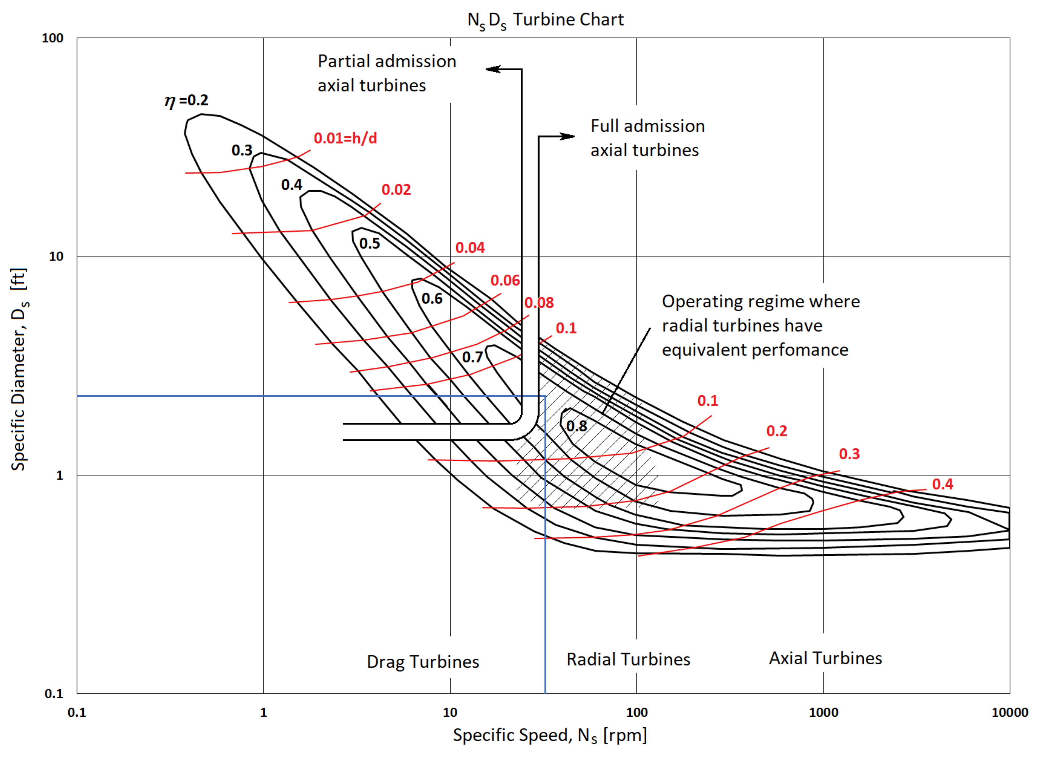
. The turbine should operate with—(i) a specific speed,
, equal to 32.3 rpm imposed by the coupling with the electric generator; (ii) a specific diameter,
, equal to 2.3 ft imposed by the dimension of the pipeline into which the machine should be mounted; (iii) a flow coefficient,
, equal to
. With these non dimensional parameters, we checked on the Balje’s diagram (
Figure 1) which could be the best configuration for this application. The Balje’s diagram suggests a full admission single stage axial turbine. This is considered a good choice, since the axial configuration allows a simpler insertion of this system in a pipeline in place of a Pressure Reduction Valve (PRV). Furthermore, the axial configuration allows a simpler integration of the magnets of the direct drive generator inside the rotor of the turbine since, actually, the turboexpander was supposed to embed the electric generator rotor [
47,
48,
49,
50], aiming at a robust design, with as few as possible components and avoiding any loss in the mechanical transmission of the torque. This configuration made unfeasible the use of conventional multistage axial turbomachines or centripetal turbines.
Furthermore, a significant advantage of the proposed procedure is that it can be used even when the operating conditions goes outside the conventional range, where the models available in the literature (e.g., References [
51,
52,
53,
54]) fail.
Finally, in order to make considerations about the impact of this technology, its application to a real gas pipeline, namely the Trans Austria Gas Pipeline (TAG) (Austria), has been taken into account (power absorbed by 5 compressor stations = 450 MW and annual flow rate of natural gas equal to 41 bmc/year) [
55]. It is worth to highlight that, especially in mountain areas, compressor stations are often employed to overcome a hill and back pressure control valves are installed, in order to avoid slackline. This is another kind of valve that can be retrofitted with a turboexpander technology. Depending on the pressure ratio required along the line, for example, a pressure drop after a hill or before a branching line to connect the pipeline to a CGS, different sizes of turboexpander can be selected. Taking into account geometries similar to the one proposed in this work, one can see that for small pressure drops, as in the case of a valley site down to the hill, the power recovered can be about 16.9 MW (e.g., obtained with a turbomachine characterized by
= 1.15,
= 1.06,
= 47.0); otherwise for larger pressure drops before a CGS, the generated power can easily reach 45 MW (e.g., obtained with a turbomachine characterized by
= 1.5,
= 1.39,
= 20.9). The latter is more or less half the power required by one compressor station in the TAG pipeline system, a remarkable result which confirms the potentiality of this kind of technology. Finally, considering an emission factor of 400 kg
CO2/MWh obtained by Italian national data for the last ten years [
56], the CO
2 emission reduction can reach 59,300 and 157,000 t
CO2/year for small and large pressure drop, respectively.
2. Design Methodology Overview
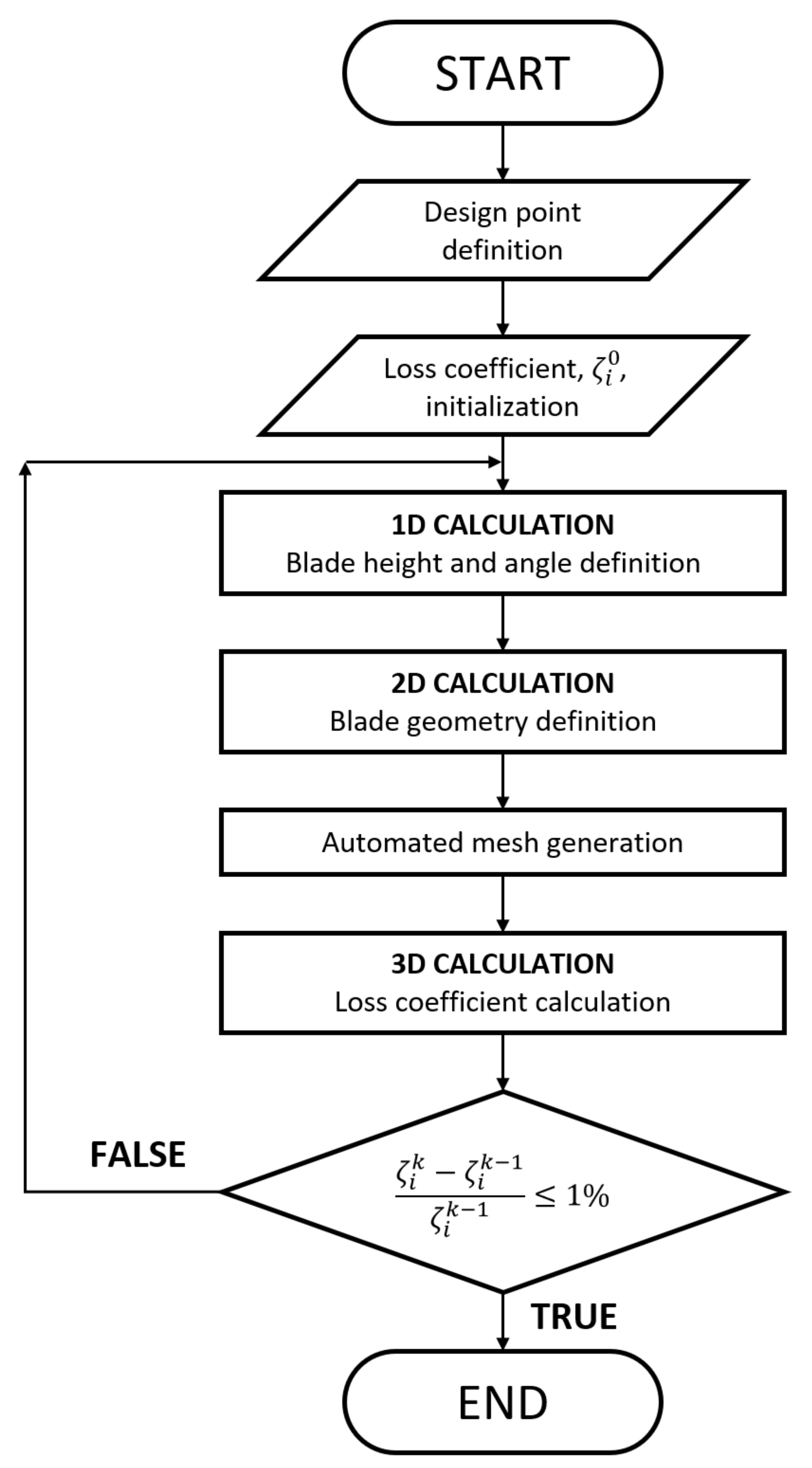
The proposed methodology can be summarized by the flow chart in
Figure 2. It begins with the definition of the turbine design point, from which the operating conditions are derived, that is, mass flow rate,
G, total pressure,
, and total temperature,
, at the turbine inlet and the pressure drop,
, across the turbine.
Loss coefficients are introduced, in order to take into account irreversibility. Actually, the very next step of the procedure involves the initialization of the loss coefficients with trial values,
. As a first guess, an ideal calculation can be performed, considering the loss coefficients equal to either 1 or 0 (depending on their definitions). After that a 1D design procedure is applied by means of a script implemented in MATLAB
®. The turbine is decomposed in its main parts (namely, the nozzle, the stator, the rotor, and the diffuser), and for each one a system of governing equations is solved. Each system of equations is composed by: the first law of thermodynamics; the continuity equation; the ideal gas law and the relations among velocity vectors according to the velocity diagrams. Thus, the one-dimensional calculation (as presented, for instance, in Reference [
54] and in Reference [
57]) provides the main operating and geometrical parameters of the machine such as the blade heights (
), the absolute and relative inlet and outlet angles (
), and the rotational speed,
N, of the machine. It is important to emphasize that the use of an embedded permanent magnet direct drive generator allows the turbine to work always at its maximum efficiency.
Subsequently, a 2D calculation is performed to define the stator and rotor blade profiles. Regarding the stator blades, their camber lines are designed according to third order Bézier curves and their thicknesses are defined according to the ones of symmetric NACA four digit airfoils. This blade design criterium was defined in order to ensure the continuity of the surface curvatures, reducing the risk of flow separations. Regarding the rotor blades, an impulse turbine technology has been chosen, by considering a modified Curtis stage layout. After having assigned all the geometric and kinematic constraints, the set of independent variables is defined by means of the genetic algorithm NSGA-II, available in the multi-objective optimization software ModeFrontier
®. The objective functions are derived by the minimization of the primary and secondary losses of the blades, and maximization of the rotor blade lift coefficient. For a fast evaluation of the force coefficients taking into account drag effects, a “one-way coupled viscous/inviscid interaction model” (see Reference [
58]) is used. This is based on the vortex panel method shown in Reference [
59] and the integral method for the solution of the boundary layer equations presented in Reference [
60]. Moreover, the optimization algorithm allows to integrate not only fluid dynamic constraints but also operating and technological ones, for instance: maximum rotation speed of the electric machine and/or the minimum thickness of the trailing edge. At the end of this step, the proposed model provides all the geometric parameters for the turbine construction.
Then, the computational domain and the mesh are automatically generated in order to minimize the time cost. This is carried out by means of a script file, (called “replay”) which is updated with the main parameters of the geometry and then run in the ANSYS ICEM CFD® grid generator. Due to the low aspect ratio of the blades, the inlet angle of the flow does not show significant variations from the hub to the tip, hence the blades are designed without twisting them along the radial direction.
The last step of the procedure is represented by a 3D RANS simulation of the flow through the turbine, which is performed in order to validate the design and evaluate the loss coefficients, to be updated and used in the next iteration ().
Actually, the calculation of the loss coefficients from the 3D simulations is carried out considering the thermodynamic characteristics of the flow evaluated as mass-weighted averages and considering that the pressure drop across the machine is the same in both ideal and real cases.
The proposed methodology is necessarily iterative since the turbine geometry depends on the loss coefficients, but these depend on the turbine geometry. The procedure stops when the generic loss coefficient,
, at the
iteration, differ less than 1%, from the value at the previous one,
(see
Figure 2).
3. Three-Dimensional Computational Fluid Dynamic Modelling
3D viscous CFD calculations are carried out by means of the commercial software ANSYS FLUENT® in order to evaluate the performance of the turboexpander. In this way, the trial values used for the loss coefficients are checked against the numerical results.
The computational domain includes the whole machine since the different numbers of stator and rotor blades do not allow the application of circumferential periodic boundary conditions.
The domain consists of three regions connected by non-conformal interfaces. Fixed and moving components are placed in different sub-domains. The numerical solution is based on both the moving and the stationary reference frames.
The manner in which the equations are treated at the interface leads to three possible approaches, all supported in ANSYS FLUENT:
Multiple Reference Frame model (MRF);
Sliding Mesh Model (SMM);
Mixing Plane Model (MPM).
Both MRF and MPM approaches are steady-state approximations and differ primarily in the manner in which data are treated and exchanged at the interfaces. On the other hand, the SMM approach is intrinsically unsteady due to the actual motion of the meshes.
In detail, the MRF model [
61] is a steady-state approximation in which different rotational and/or translational speeds can be assigned to individual cell zones. The flow in each moving cell zone is solved using the moving reference frame equations. It is worth noting that the mesh relative motion of adjacent zones is not considered by the MRF approach. Hence, the moving parts are frozen and the flow field is calculated by neglecting the relative motion of the moving zones. The MRF model is suitable in nearly uniform flow at the interface between adjacent moving/stationary zones (“mixed out”).
The SMM method is used when a time-accurate solution for rotor-stator interaction is desired instead of a time-averaged solution. Even though the SMM is the most computationally demanding, it is a good practice for unsteady flow simulations in multiple moving reference frames, especially to account for rotor-stator interaction in turbomachineries. In the SMM technique two or more cell zones are used and each of them actually slides along the grid interface in discrete steps. When the rotation or translation takes place, node alignment along the grid interface is not required.
The MPM provides an alternative to the MRF and SMM in order to simulate the flow through moving zones. In the MPM approach, a steady-state problem for each zone is solved considering the mixing plane interface between adjacent zones as a boundary where the flow-field boundary conditions are set with spatially averaged or mixed condition. This mixing keeps smooth the flow variations by means of a circumferential averaging at the interface (i.e., wakes, shock waves, separated flows), therefore yielding a steady-state result. Despite the approximation of the MPM model, the time-averaged flow field is acceptable in a wide range of flow field conditions.
CFD Model Validation and Grid Sensitivity Analysis
In order to assess the 3D CFD and, in particular, to verify the best approach for the analysis of the rotor/stator interaction, a reference case [
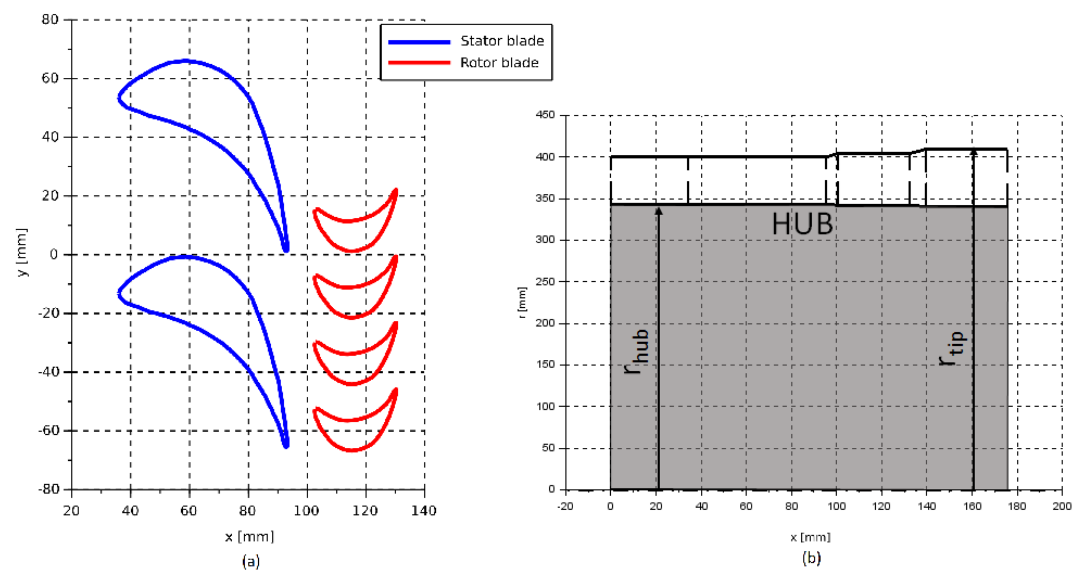
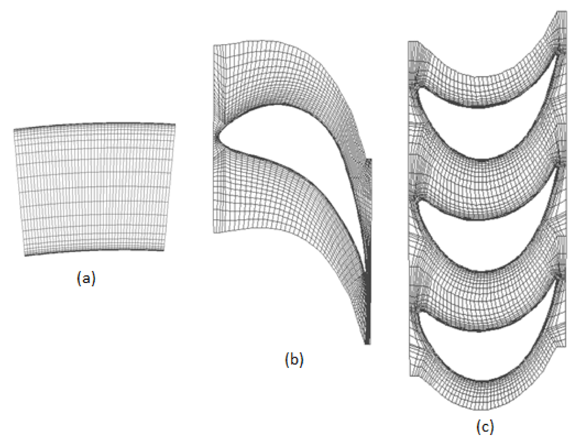
62] has been considered for validation. The turbine under investigation is the air turbine stage of the Institute of Thermal Engineering (ITC) of Lodz, model TK9-TW3 [
63] which is a typical HP turbine stage. It operates with short-height cylindrical blading and aft-loaded stator profiles with the following characteristics: span/chord
(stator) and
(rotor), pitch/chord
(stator) and
(rotor), span/diameter
(stator and rotor). In
Figure 3 the turbine stages are reported on the blade-to-blade (a) and the throughflow planes (b).
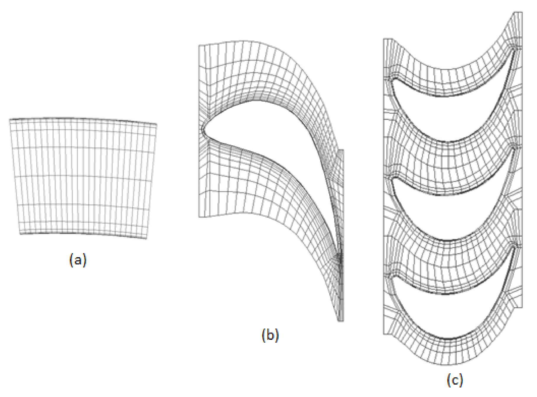
For each region of the domain, a customized structured multi block mesh has been generated, taking into account both the local geometry and the flow conditions.
In order to capture directly the wall boundary layer effects (), the first cell height has been kept as small as possible however avoiding problems of negative volumes. Furthermore a settling chamber is added downstream of the computational domain in order to prevent any convergence problem related to “reversed flow”.
The standard
turbulence model [
64] has been considered according to several previous numerical investigations [
65,
66,
67,
68].
The turbine under investigation operates with a mass flow rate G = 4 kg/s at an inlet static pressure = 1 bar and an inlet temperature = 320 K. The outlet pressure is = 0.9 bar. The rotational speed is N = 1450 rpm.
In order to simulate these operating conditions a mass flow rate has been imposed at the inlet section of the computational domain. At the outlet section, a pressure-outlet boundary condition has been imposed. At the inlet section, the turbulent intensity is set equal to 5% and the turbulent length scale equal to 1 mm. A grid independence study has been carried out using the moving reference frame model implementing the MRF approach. The study has been performed doubling each time the number of nodes on each edge. The total-to-total efficiency has been considered as the control parameter. In
Table 1 the study is resumed, whilst in
Figure 4,
Figure 5 and
Figure 6 the meshes used in each simulation are shown.
The grid independence study highlights that 1M cells discretization is able to achieve the requested accuracy. The MPM approach showed unstable behaviour of the numerical solution hence it has been discarded.
For both the Moving Reference Frame Model and the Sliding Mesh Model, the first parameter that has been analysed is the pressure drop across the turbine. Particularly, for the MRF the pressure drop is equal to 0.091 bar, whilst for the SMM is equal to 0.095 bar, with an error, computed against the experimental data, of 9% and 5%, respectively.
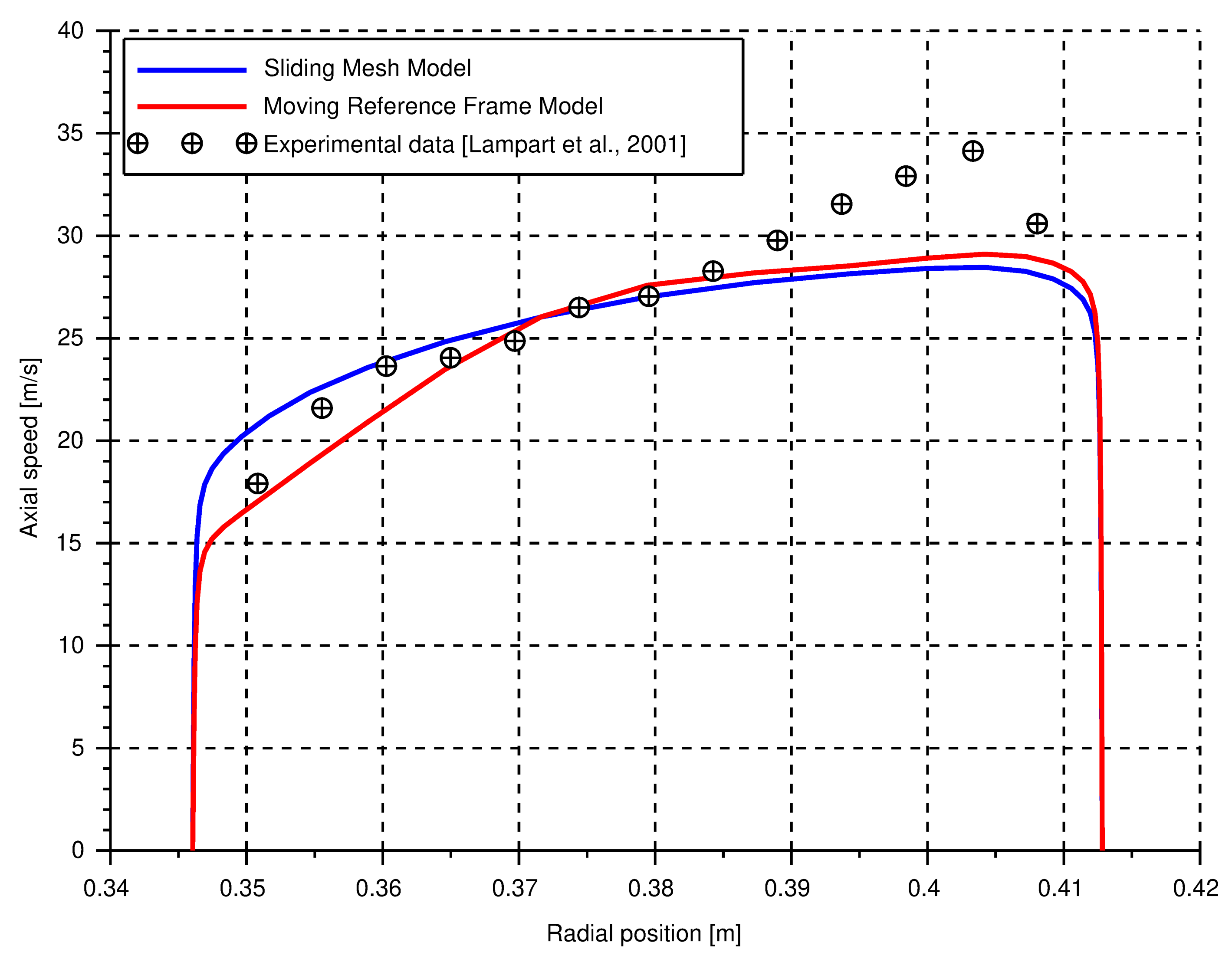
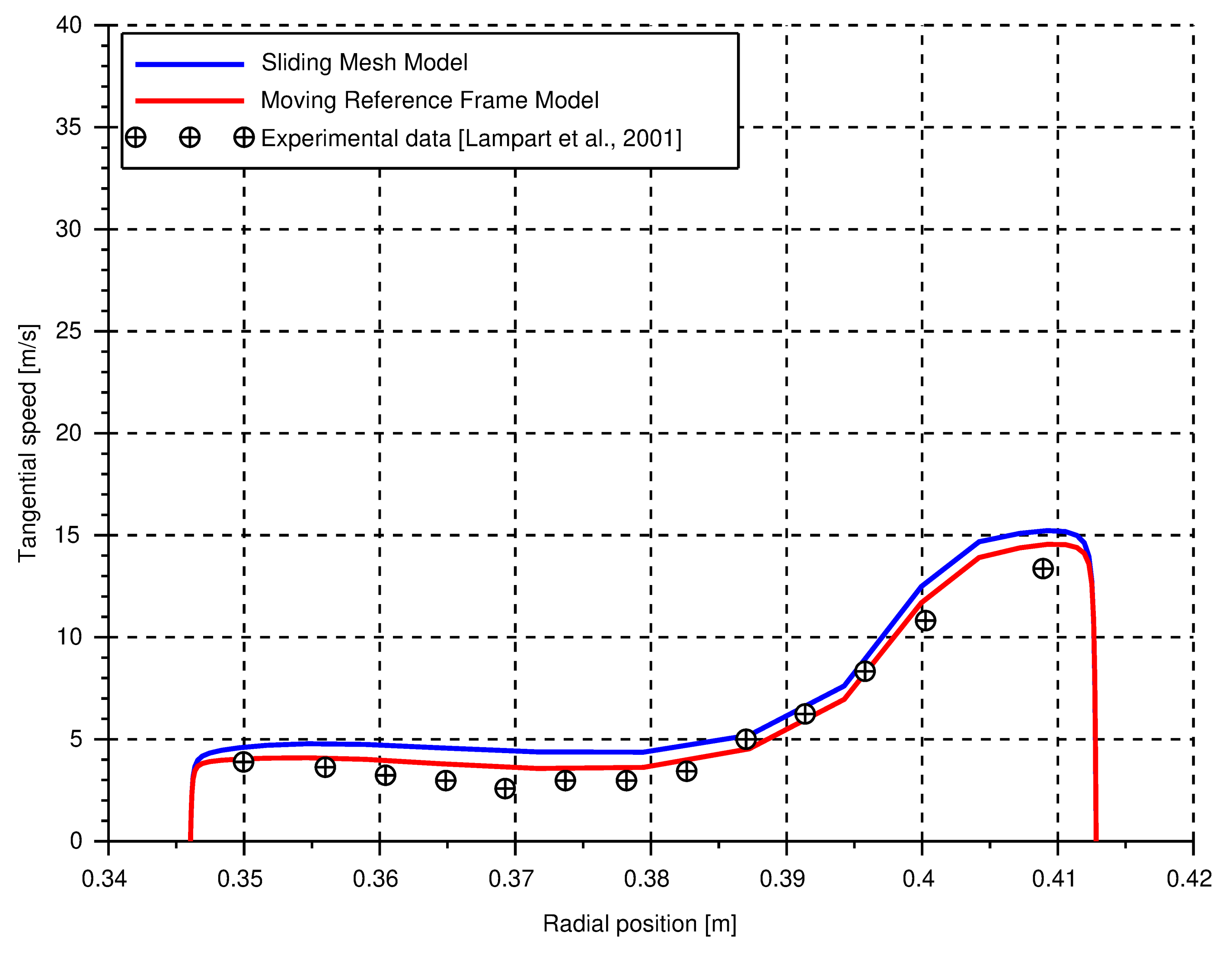
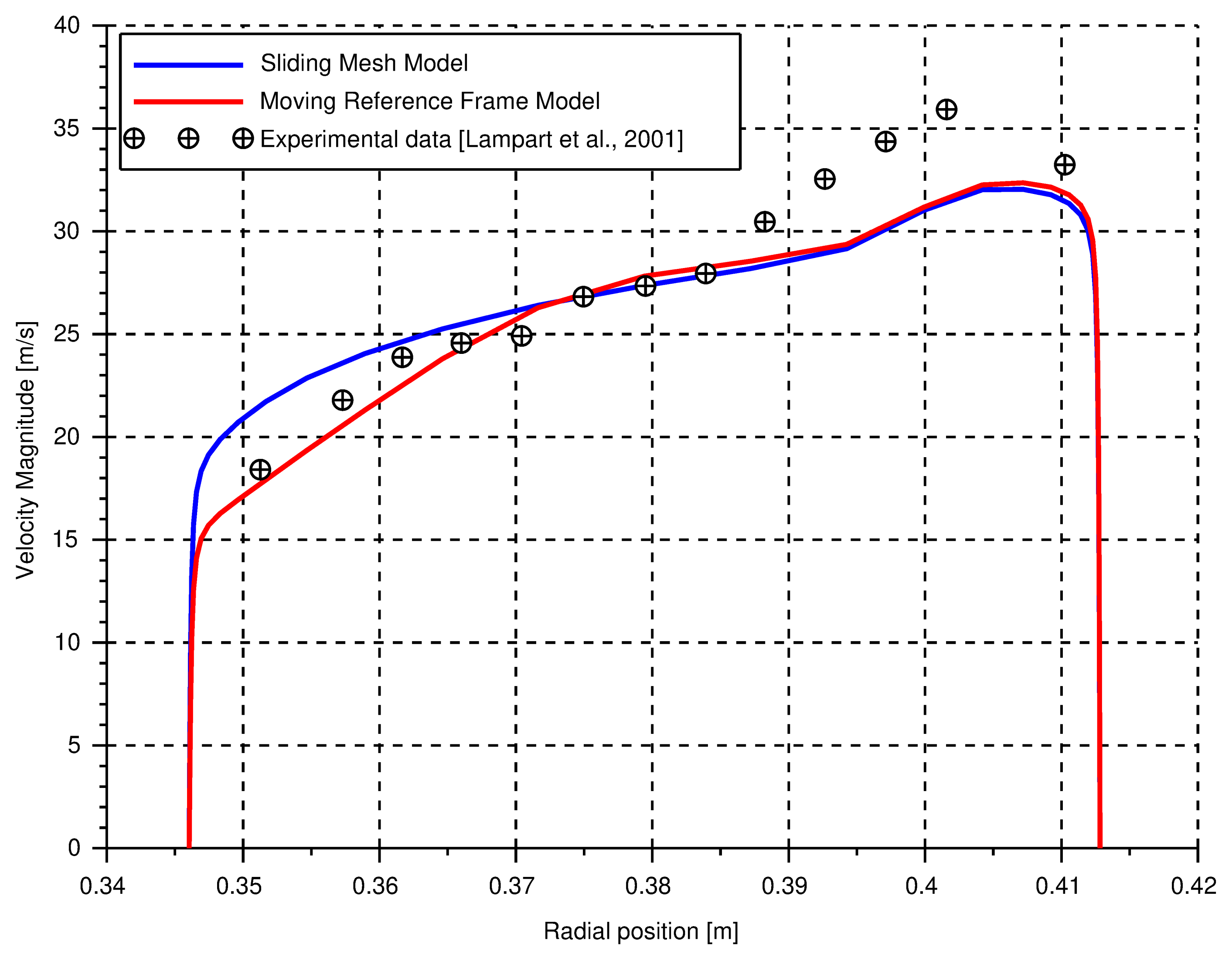
Another comparison has been carried out considering the absolute velocity components (axial, radial and tangential) in a section located at 135% of the axial chord downstream of the rotor trailing edge, that is the distance corresponding to the location of the measuring probe at the experimental facility (
Figure 7,
Figure 8 and
Figure 9).
As reported in
Figure 7,
Figure 8 and
Figure 9 and from
Table 2, MFR and SMM provide approximately the same results since the Mean Square Error Percentage (MSEP) shows minimal differences between the two models. Particularly, the tangential speed shows the best agreement between experimental data and the computational results. The value of the axial speed at the tip is underestimated by both the models, whilst at the hub the axial speed is underestimated or overestimated if the MRF or the SMM are used, respectively. The absolute speed differences can be found at the hub and at the tip. In detail, at the hub the simulation results match the experimental trend, whereas the models underestimate the axial velocity at the tip. Indeed at the hub it is possible to observe the same trend as the axial speed, whilst at the tip the simulation tends to underestimate the value of the absolute speed.
Even though the SMM gives the best results in this assessment, it is extremely time consuming with respect to MRF. Hence, the MRF model represents the best compromise in terms of accuracy and computational effort.
4. Case Study
The proposed methodology has been applied in order to design a single stage axial turbine to be used in substitution of a pressure reduction valve, exploiting the pneumatic energy associated to its pressure drop. The application taken into account requires that the turbine operates with a loading factor, , at least equal to , an expansion ratio, , equal to and a flow coefficient, , equal to .
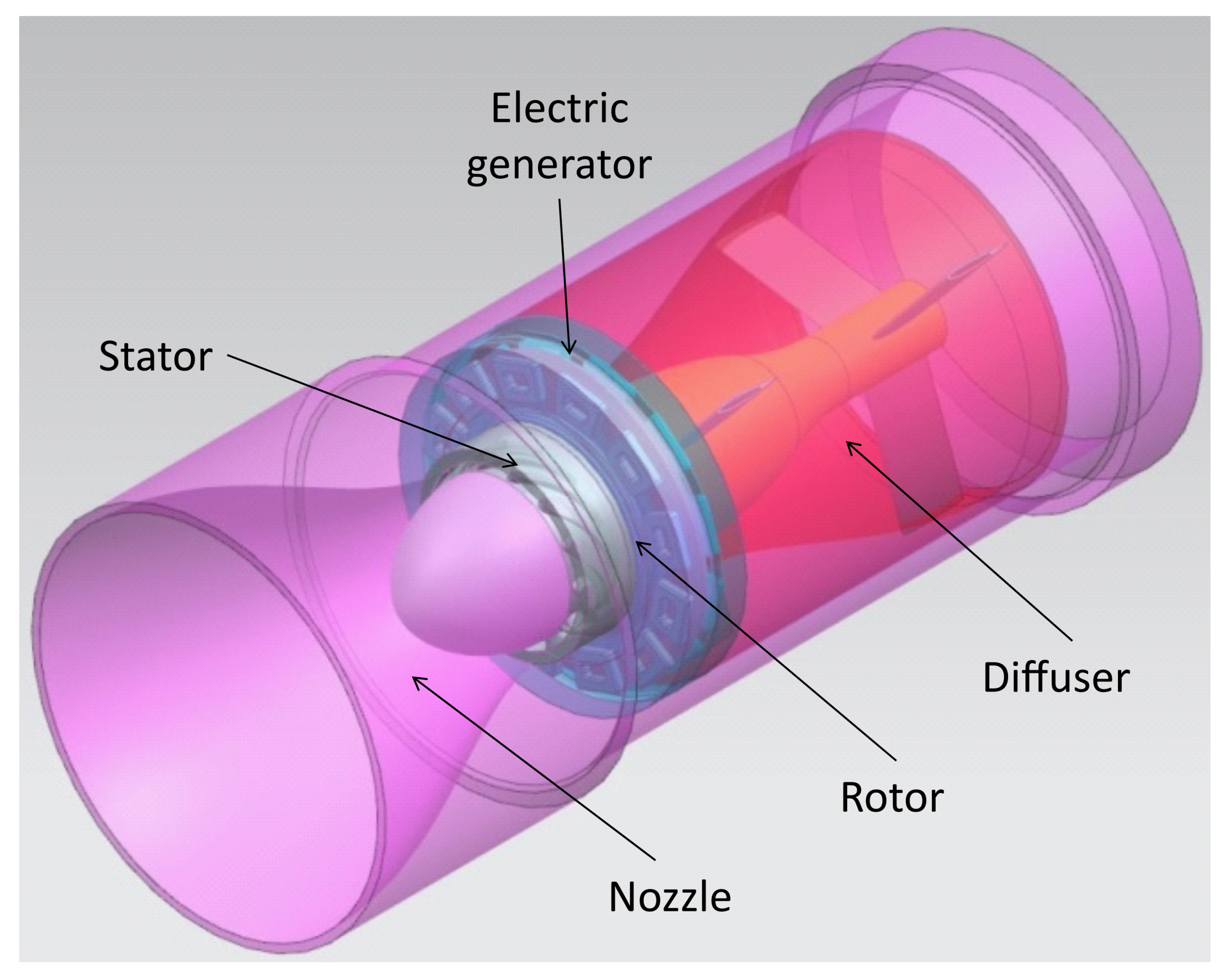
The turbine under investigation is composed by a nozzle, a single stage axial turbine, and a diffuser (
Figure 10). In the 3D CFD calculation, the computational domain includes all the parts of the machine, considering air as an ideal gas. Furthermore, the design involves both the loss coefficients of the nozzle,
, and of the diffuser,
.
Following the procedure, described in the previous chapter, the relative error becomes quickly lower than 1% already at the 3 rd iteration as shown in
Table 3.
As described in the flow chart of the iterative procedure (see
Figure 2), the process is initialized under the hypothesis of an ideal machine without losses.
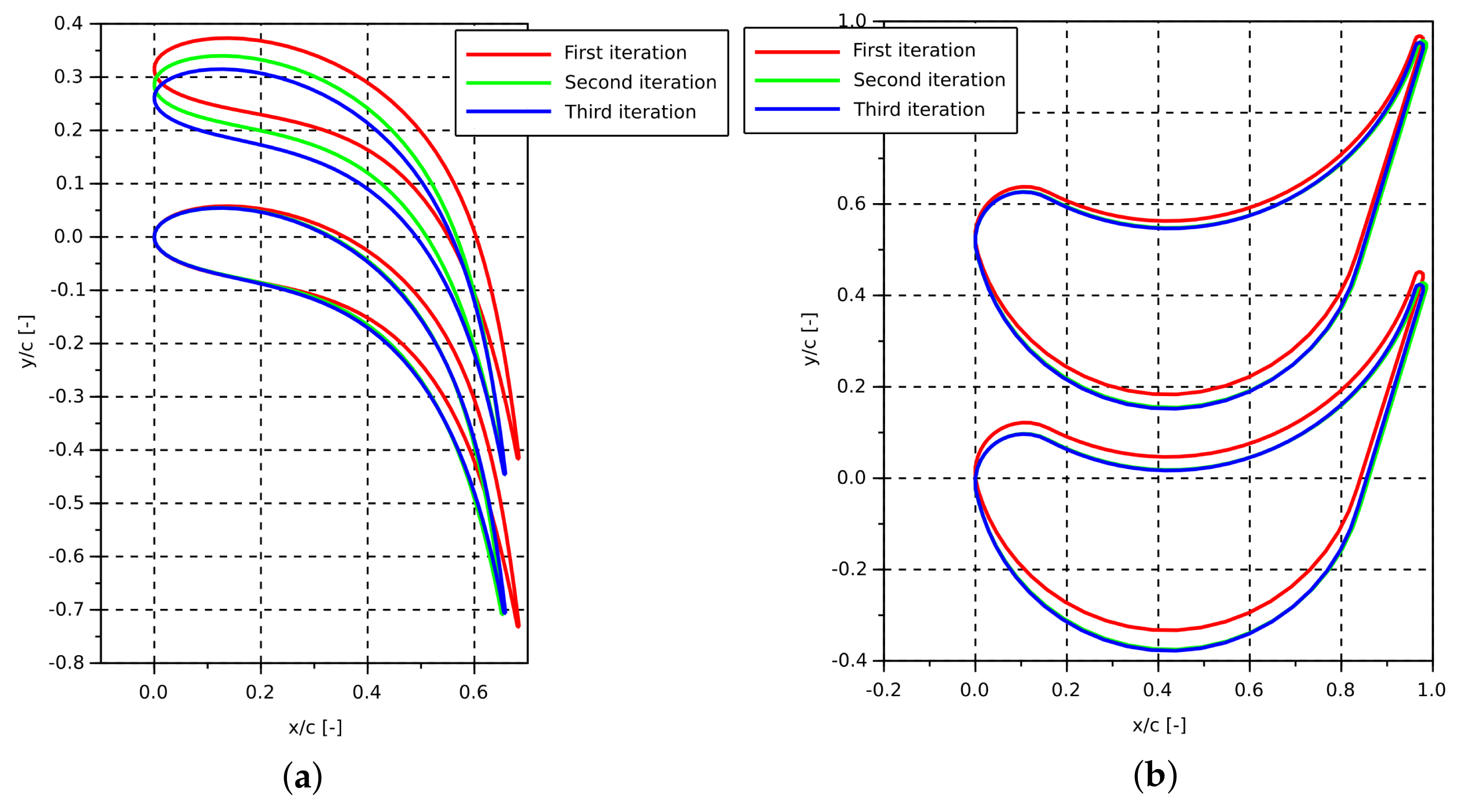
The variation of the loss coefficients during the iterative procedure is reflected by the change of the machine geometry, and specifically of the heights (
Table 4) and airfoil shapes of both stator and rotor blades (
Figure 11). Looking at
Figure 11, one can see that the substantial variations occur to the stator blade profiles going from the first to the third iterations. Moreover, the turbine rotational speed (
Table 5) is also modified in order to preserve the optimum working conditions (namely, inlet flow velocities aligned with the inlet blade angles).
Indeed, as shown in References [
54,
57], the loss coefficients affect the thermodynamic properties of the flow at each considered section of the turbine. According to the continuity equation, for increasing losses, the pressure drop increases, whereas the density decreases as well as the velocity.
Once the geometry of the machine has been defined, a simulation has been carried out with a finer mesh in order to study in detail the fluid dynamic behaviour of the machine. The mesh density has been selected by means of a mesh sensitivity study, which is not reported here for the sake of brevity.
The results of this last simulation (the one characterized by the finest used mesh) are summarized in
Table 6 together with those obtained with the starting coarse mesh, for comparison. Actually, the mesh used during the convergence procedure underestimates the performance of the turbine. Furthermore, from
Table 6 it is possible to observe that the turbine designed with the proposed tool allowed us to reach the desired results. Indeed, under the design working conditions in terms of flow coefficient (
) and expansion ratio (
), the turbine gives a loading factor,
, more than twice the minimum expected value of
(
Table 6).
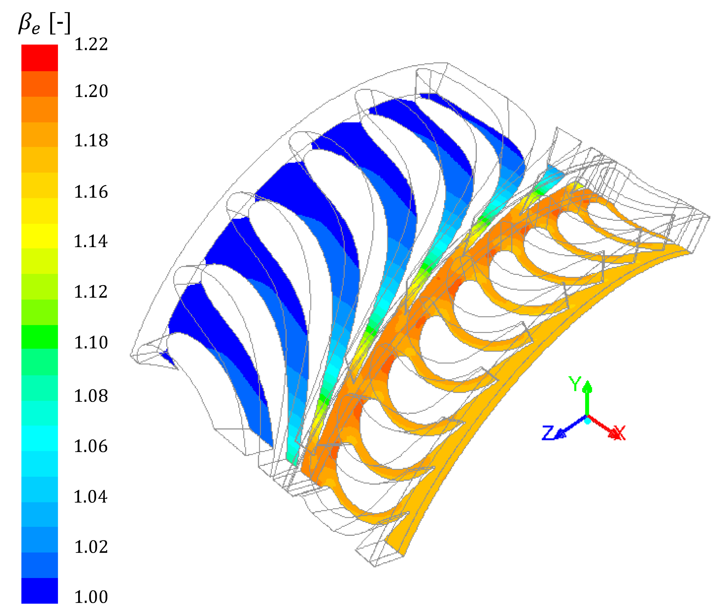
Figure 12, which represents the contours of the expansion ratio at the hub of the stator and rotor blade passages, confirms the impulse behaviour of the turbine: the entire pressure drop available is elaborated by the stator, whilst across the rotor the flow experiences only a minimum pressure drop essentially caused by distributed losses.
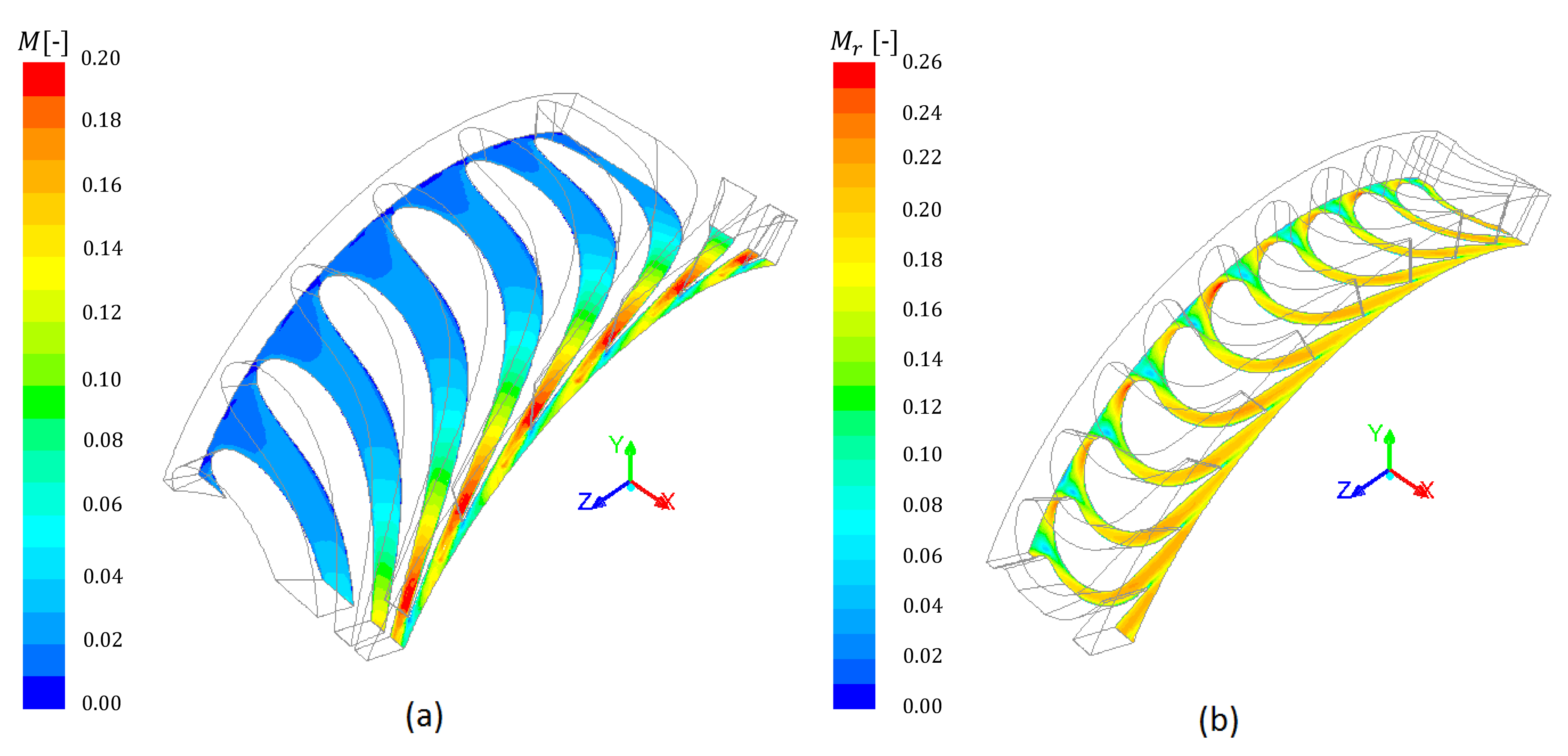
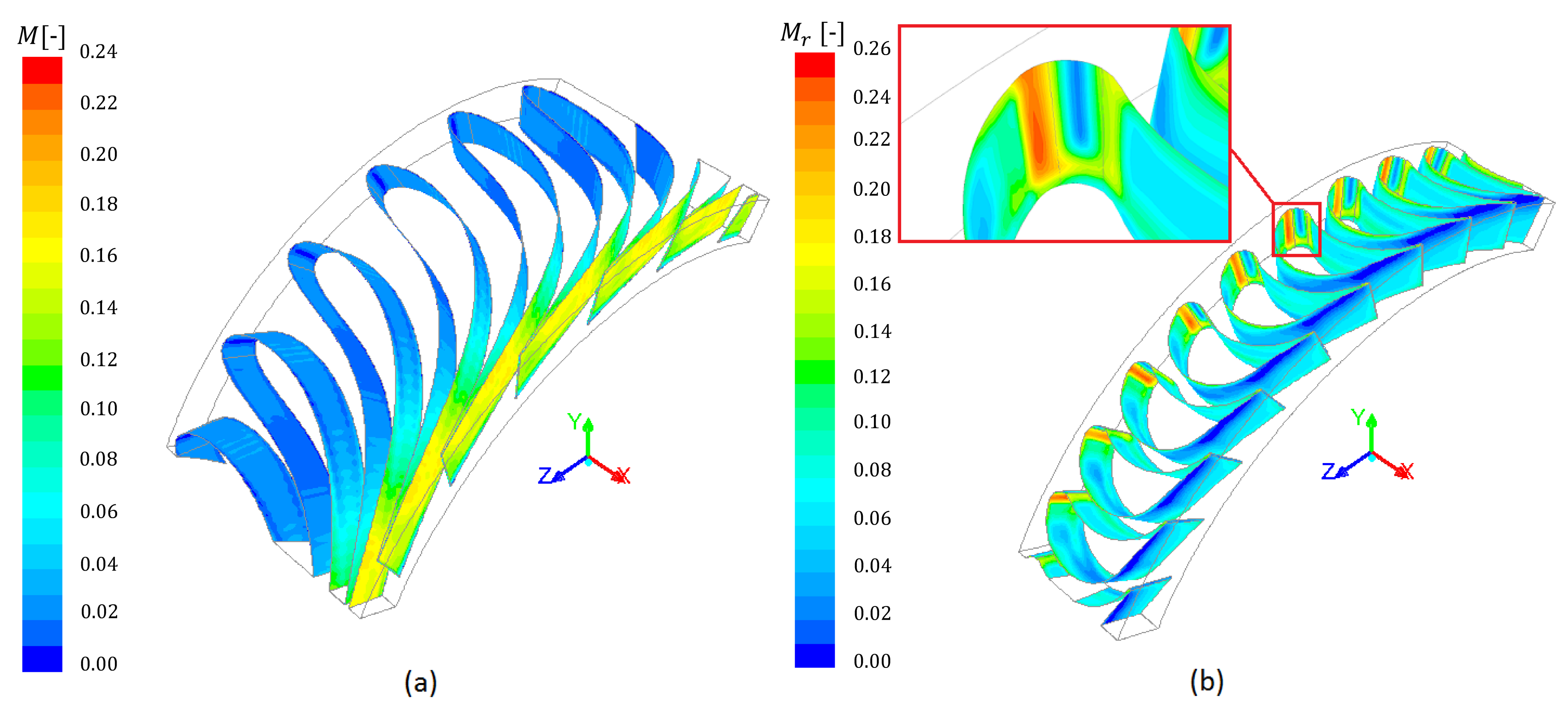
This behaviour is also confirmed by
Figure 13, which reports the absolute and the relative Mach number contours for the stator and the rotor, respectively. Again, the absolute Mach number in the stator evidences the flow acceleration in the stator whereas the relative Mach number shows only minimum variations especially after the leading edge. Due to the impulse behaviour of the rotor, actually the work extraction is mainly due to the change of the flow direction rather than its acceleration, which is negligible.
The Mach number distribution is also analysed around the blade surfaces, in order to verify the presence of high pressure gradient zones which can determine flow separation (see
Figure 14). The Mach number distribution is regular around the stator blades, whilst the relative Mach number distribution around the rotor blades shows a high gradient in the leading edge zone.
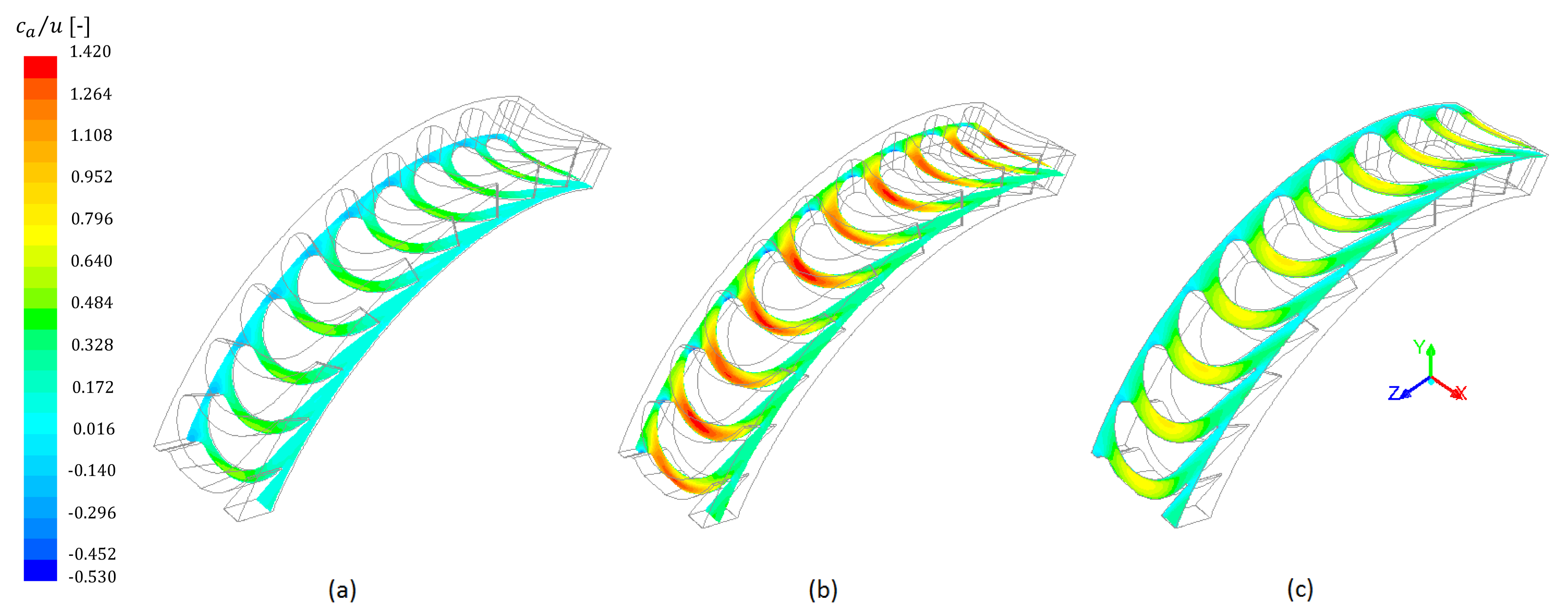
The ratio between the axial and the tangential velocities at the mid and tip of the rotor is shown in
Figure 15. The signature of the flow separation is the negative value of the axial velocity registered at the blade leading edge. This phenomenon takes place because of the particular design of the rotor blade. Indeed, in the connection of the leading edge arc with the pressure side and the suction side, only the continuity of the first derivative is preserved, whereas the continuity of the second derivative is not guaranteed.
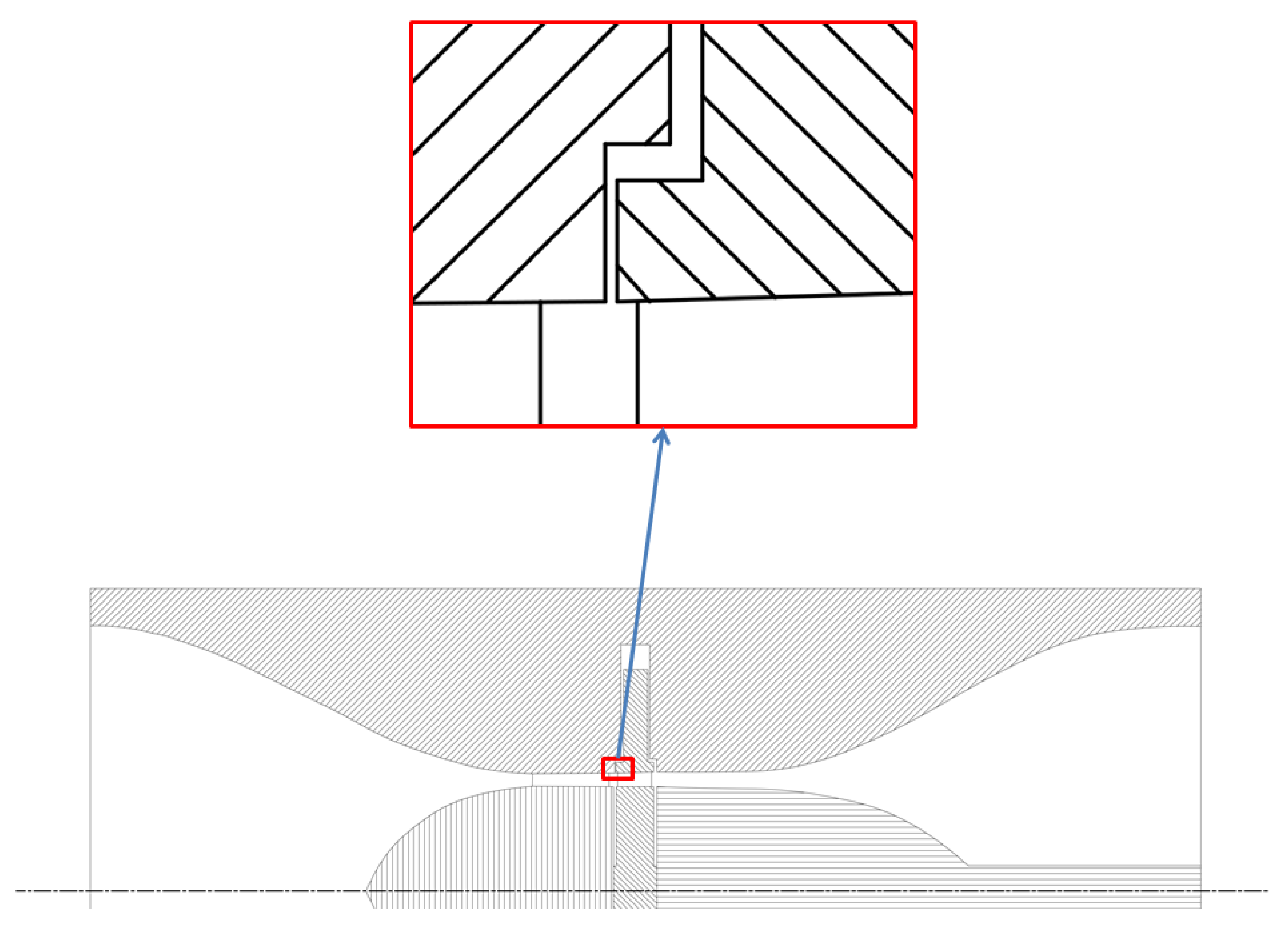
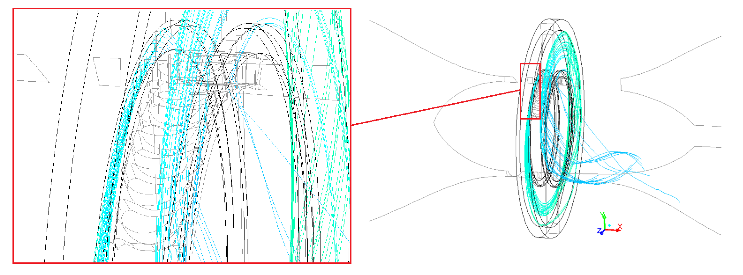
Another issue which influences the global efficiency of the designed machine is represented by the leakage through the clearance between the rotor disk and the casing. In the preliminary steps, in order to minimize this problem, the inlet section for the leakage mass flow (
Figure 16) was kept as lower as possible, compatibly with technological issues relative to manufacturing. Nevertheless, a volumetric efficiency exists and influences the performance of the machine. In
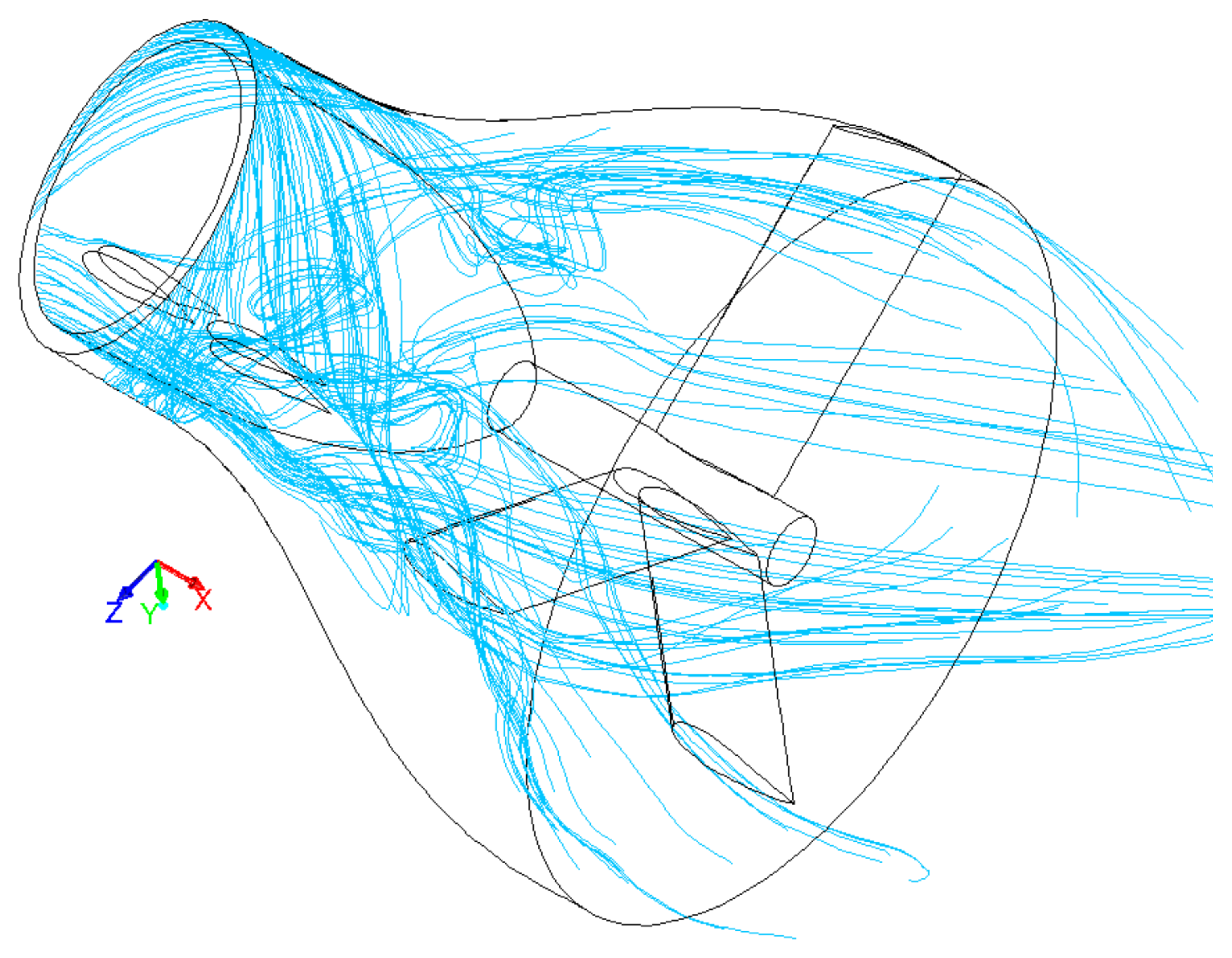
Figure 17 it is shown how the streamlines just under the tip of the stator blades bypass the rotor blades flowing through the tip clearance between the rotor disk and the casing, determining a device work loss.
Also the diffuser seems to have a bad influence on the global efficiency of the machine according to its loss coefficient,
= 0.1890. Actually, as shown in
Figure 18, the streamlines are very irregular pointing out the kinetic energy losses. This is due to axysimmetric profile of the diffuser, especially when the available cross section area rapidly increases. Indeed, a smoother passage area increase is expected in order to improve the diffuser efficiency, but the available axial size constraint does not allow to modify the diffuser geometry. After this detailed insight in the fluid dynamic behaviour of the designed machines, it is evident that margins exist for a further improvement, but this will be subject of a next work.
5. Conclusions
For a sustainable development of industrial processes, the energy recovery can be an effective strategy. Under this framework, a design procedure for turboexpanders has been developed, which is characterized by a high level of automatization and a fast convergence toward the optimal solution. In order to validate this procedure, this was applied to an innovative turboexpander characterized by a high specific speed (with an embedded permanent magnet direct drive generator) thought for substituting a Pressure Reduction Valve (PRV) in a pipeline. The design requirements were specified in terms of maximum allowable expansion ratio () and flow coefficient (), while achieving the highest possible turbine loading factor (). The design procedure is iterative and based on the following four steps:
a one-dimensional calculation aimed at the evaluation of the main geometric (blades angles and heights) and operating (output power, rotational speed and efficiency) parameters of the turbine;
an optimization algorithm based on a two-dimensional viscous/inviscid interaction technique in order to evaluate both stator and rotor blade shapes;
set up of a script file, based on the geometry resulting from the previous two steps, which is read by the mesh generator software and which allows the automatic generation of the mesh;
a three-dimensional CFD simulation performed in order to verify the design in terms of performance and loss coefficients.
The need to adopt an iterative procedure lies in the fact that when the design process starts, the loss coefficients to be used in the one-dimensional calculation are not known, hence a hypothesis on their values has to be done. If the supposed values of the loss coefficients are equal to the ones resulting from the 3D CFD simulation, convergence is reached, otherwise the one-dimensional calculation is updated and the iterative procedure continues. By means of a test case, an assessment of the CFD model as been performed. In particular, the attention was focused on the mesh density to be used during the iterative procedure, which should be a right compromise between accuracy and computational costs. Furthermore, the possible models for dealing with rotor/stator interaction have been investigated and then, the Multiple Reference Frame model has been selected to be used in the design methodology. The iterative procedure allowed us to reach a satisfactory turbine design after only three iterations. When the design was completed, a fine mesh has been generated in order to obtain the final results.
Furthermore, the results show that the final turboexpander design is characterized by a loading factor ( = 1.800), which is more than twice the minimum expected value (0.8262). Finally, an insight into the flow field has been carried out by investigating the contours of the Mach number and the streamlines across the turbine stage. The former points out small regions close to the rotor blade leading edges where flow separation occurs; the latter evidences that the diffuser profile can be improved to minimize the kinetic energy losses.

 ,
, 


