Abstract
The use of compensation networks increases the power transfer capability of inductive power transfer (IPT) systems in the battery charging process of electric vehicles (EVs). Among the proposed topologies, the Series-Series (SS) and the LCC networks are currently in widespread use in wireless battery chargers based on IPT systems. This paper focuses on the study of the behavior of both compensation topologies when they are detuned due to the tolerances of their components. To compare their performances, a Monte-Carlo analysis was carried out using Simulink and MATLAB. The tolerance values, assigned independently to each component, fall within a [, 20] % range according to a normal distribution. Histograms and scatter plots were used for comparison purposes. The analysis reveals that the LCC network allows a tighter control over the currents that flow through the magnetic coupler coils. Moreover, it was found that the increments in those currents can be limited to some extent by selecting capacitors featuring low tolerance values in the LCC compensation. Nevertheless, the SS network remains an appropriate choice if size and cost are essential constraints in a given design.
1. Introduction
The increasing trend in greenhouse gas emissions elucidates the need for a transition to a decarbonized energy system. In this scenario, electric vehicles (EVs) become a clear alternative for internal combustion engine automobiles. Since EV operation does not cause direct emissions, the air pollution from road transport can be significantly reduced if clean energy technologies are adopted. Nevertheless, some aspects concerning the battery pack, such as its charging process, need further investigation.
At first, the EV battery charging process was accomplished by means of conductive chargers. However, the need for a mechanical connection between the transmitter and the receiver increases the electrocution hazard. In these systems, the user needs to touch the transmitter connector. This, in a moist environment or in the case of insulator deterioration, may result in an electrical shock. Wireless Power transfer (WPT) systems diminish remarkably this danger because of the absence of mechanical connectors. In addition, there exist a galvanic isolation between the subsystem installed in the parking space (ground assembly, ) and the one located in the vehicle (vehicle assembly, ). The acronyms and were taken from the standard SAE-J2954 for the recharging of light-duty EVs [1]. These advantages, along with the minor maintenance required, have promoted extensive research in this type of systems.
Near-field WPT systems can be classified according to the electromagnetic phenomenon on which they are based. Capacitive power transfer (CPT) systems use the electric field coupling to transmit power between two conductive surfaces separated by a dielectric medium. Their most common configurations consist of conductive plates with ring and square geometries connected to frequency compensation networks. One or more plates are located at both the transmitter and receiver sides of the system, having as a result two resonant subsystems [2,3,4,5].
In inductive power transfer (IPT) systems the conductive surfaces on the transmitter and the receiver sides are replaced by coils. Thus, the magnetic field is the responsible for the power transferred by means of the induction phenomenon. Coil geometries have been widely discussed, being rectangular, circular and double-D coils the most extended configurations [6,7,8]. Nonetheless, other coil topologies have also been proposed, as the taichi, flux-pipe, cross-shape, hexagonal or the so-called quad D quadrature [9,10,11,12,13].
There exist some advantages in the use of CPT systems. For example, the presence of nearby metal objects results in lower losses since the induced eddy currents are significantly reduced [14]. In addition, they have a lower weight and cost, as well as a smaller magnetic interference with other devices [15]. However, their operation at air-gap distances of about 150 mm results in small capacitances. Therefore, either high operating frequencies (about 1 MHz) or compensation networks with very large inductance values are needed to reach relatively high-power levels [4,16]. Yet another disadvantage is the field shielding. It is harder to attenuate the unwanted electric field emissions than those of the magnetic field. Consequently, CPT systems are more prone to unsafe field emissions than IPT systems [14].
One of the main advantages of inductive over capacitive power transfer is its higher power density. Moreover, high-power transmissions can be achieved at lower operating frequencies with a higher system efficiency. This, along with the easier shielding of the magnetic field, have made IPT technology to stand out as the prevailing choice for WPT charging of EVs batteries [14].
Compensation topologies of IPT systems have been studied in depth, particularly in the grid-to-vehicle (G2V) power transfer direction. Originally, four basic structures were proposed. They are characterized by a compensation capacitor connected, either in series or in parallel, with the coils of the magnetic coupler [17]. Each topology is labeled with two letters. The first one depends on the association of the capacitor with the coil in the (primary side). When it is connected in series, an S is assigned. On the contrary, if a parallel compensation of the coil is chosen, then a P is used. The same occurs with the second letter, which indicates the type of connection used in the (secondary side). The Series-Series (SS) compensation stands out among these four basic topologies. Unlike the other three options, its resonance frequency is independent of variations in the magnetic coupling coefficient (k) or in the load connected to the receiver side [18]. However, the transmitted power increases greatly with the misalignment between coils, which may lead to unsafe operation [19].
In order to overcome the disadvantages of the basic compensation topologies, more complex structures have been proposed [20,21,22]. For example, the use of a parallel compensation in the requires a large inductor on its corresponding DC side. Its aim is to ensure that the rectifier works under continuous conduction mode [23]. Consequently, the size and the cost of the electronics are increased. However, if the coil is connected in series with the AC side of the rectifier, the required inductance value significantly reduces. As a result, an LCL network is obtained [23,24].
Variations of this last structure can be found in the literature [25,26]. One of the most accepted topologies is the so-called inductor-capacitor-capacitor (LCC) compensation [27]. The extra coils in an LCL compensation must have the same impedance as the coils in the original magnetic coupler for a perfect tuning condition. In the LCC topology a capacitor is connected in series with the coupler coil, achieving its partial compensation. As a result, the equivalent impedance is reduced and hence the required self-inductance of the added inductor.
Apart from the double-sided LCC compensation (an LCC network placed both on the and the sides), other topologies have been proposed [28,29]. One of the most extended configurations is the LCC-S topology. It consists of an LCC compensation on the side and a series compensation on the side. The aim is to reduce both the size and the cost in the whereas a current-source behavior is still achieved under variations in load and k [30,31,32,33].
SS and double-sided LCC configurations are currently the most extended topologies, especially when a bidirectional power flow is required. Both configurations exhibit a current-source behavior at the receiver output for a given constant voltage at the transmitter side. Nevertheless, their performance may differ significantly when deviations from the operating point occur. With the aim of establishing the differences and similarities between these two structures, some comparison studies have been reported. In [19], Li et al. analyzed the effects of variations in the coupling coefficient, load and self-inductances of the coils. Zang et al. focused on the distortion that occurs in high-power strongly coupled IPT systems () due to coupled harmonics in [34]. A comparison between SS, parallel-parallel (PP) and LCC topologies was performed by Mohamed et al. in [35]. Finally, Lu et al. evaluated the effects that component tolerances have on the efficiency and output power of an LCC-compensated system in [36].
This paper focuses on the study of the detuned SS- and double-sided LCC-compensated IPT systems because of the tolerances of their network components. First, a mathematical analysis of both tuned topologies is developed to highlight their main characteristics and expected behavior. Secondly, a Monte-Carlo analysis is performed for each topology under the same load and k conditions. In each simulation, the tolerances of the compensation components vary within the [, 20] % range according to a normal probability distribution. Histograms and correlation plots are used to perform a multivariate analysis. The aim is to determine to which extent the simultaneous variation in the values of the different components compromise the system performance.
The paper is structured as follows: The mathematical analysis of the two electrical circuit models under consideration is developed in Section 2. Section 3 describes the setup of the corresponding simulation models, while the simulation data are analyzed in Section 4. Finally, the conclusions drawn from this work are discussed in Section 5.
2. Mathematical Modeling of an IPT System with SS and LCC Compensation Networks
With the aim of highlighting the particularities found in both topologies, the mathematical expressions for the SS- and the LCC-compensated magnetic couplers are derived. The analysis is focused on the general scheme of an IPT system depicted in Figure 1. The power transfer from the DC link located at the to the is performed by means of an inverter, a compensated magnetic coupler and a rectifier. In turn, the battery pack may either be connected directly to the rectifier output or through an optional DC-DC converter. This last stage, represented in dashed lines, may be added for regulation purposes. If it is ommited, the rectifier DC output voltage, , matches the battery voltage, . However, when the DC-DC converter is placed, and are usually different DC voltages.
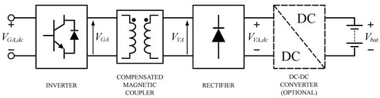
Figure 1.
Block diagram of an IPT system featuring an optional DC-DC converter for regulation of the charging process.
It is a common practice to replace the rectifier, the optional DC-DC converter and the battery pack with an equivalent resistance [28,30]. This resistor is connected to the side of the compensated magnetic coupler. As a result, the model simplifies and a linear system that depends on the output voltage of the inverter, , is obtained. However, the expression for the equivalent resistance varies for the SS and LCC topologies. Furthermore, the influence of on the currents flowing through the coils of the magnetic coupler cannot be directly obtained.
To get around this limitation, the mathematical modeling presented in this work follows the analysis adopted in [19,34,37]. It relies on the voltages and in order to describe the behavior of the compensated magnetic coupler. Thus, the use of an equivalent resistance is avoided, and the analysis can be carried out using the original scheme shown in Figure 1. An additional advantage of this approach is that the resulting equations are useful for a bidirectional power flow.
Regardless of the selected procedure, some important assumptions must be taken into account. First, all the non-linear devices in the inverter, the rectifier and the optional converter must behave as ideal components. For example, the switching dynamics and losses in transistors and diodes are neglected. Secondly, the self-inductances in the magnetic coupler must be independent of both the misalignment between coils and the transmitted power. Finally, another important assumption addresses the continuous operation mode of the rectifier. This last assumption is strictly necessary only in the case of using the equivalent resistance. However, if this condition holds also true for the chosen approach, the waveform of the voltage at the rectifier input is square-shaped. In this case, the expression for is simplified, being the amplitude of its h-th harmonic [38]:
The same equation holds true for a square wave at the inverter output, which leads to the following expression for the amplitude of the harmonic of :
2.1. Mathematical Model for an SS-Compensated Coupler
In order to model the magnetic coupling of the IPT system, the magnetic coupler shown in Figure 1 is substituted by its T equivalent circuit. The resulting electrical model for the SS topology is shown in Figure 2. Here, and are the self-inductances of the and coils, and and are the corresponding compensation capacitances. The parasitic resistances of the and coils ( and , respectively) are included. To express the mutual inductance of the magnetic coupler, the equation is used.
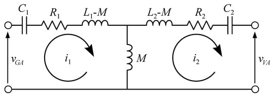
Figure 2.
Equivalent circuit of an SS-compensated coupler.
By applying the superposition theorem, the effect that voltages and have over the currents and can be studied from the analysis of two separated circuits. In each case, either or is taken as a short circuit, remaining the other unaltered. Consequently, two systems of differential equations in the time domain can be obtained. Thus, the contribution of and to the currents and can be calculated independently. Taking as a short circuit, the equations that express the influence of on and are:
where the subscript in the currents denotes the dependency of the currents on . Likewise, the influence that has on and can be obtained from the following equations:
where the lower-case letters are used to express instantaneous voltages and currents. The subscript shows the dependency of the currents on .
The corresponding frequency-dependent equations can be obtained by applying the Laplace transform to their time-domain counterparts given by (3) and (4). Solving the equations in the phasor domain for the two currents yields the following solutions:
where upper-case letters express the frequency-dependent terms. Voltages and currents are related through the admittances which, in turn, can be expressed in terms of the impedances and :
When the imaginary parts of and become zero, the reactances of the coils are compensated by the capacitors and the circuit is perfectly tuned. This condition leads to the definition of the resonant frequency, :
By analyzing (6), it can be seen that depends on the load because of the voltage . Therefore, the current-source behavior is, in principle, not achieved. However, the terms and become negligible at the resonant frequency and the dependency on virtually vanishes. For this reason, the desired current-source behavior at the rectifier input is a reasonable approximation for an SS compensation topology under resonance conditions. In addition, if the parasitic resistances and are neglected, the output current on the secondary side will be totally load-independent.
In that case, if all the harmonic components apart from the fundamental one are neglected (i.e., and ), the expressions (5) and (6) simplify to:
Thus, if the power dissipated in the system is neglected, the apparent power of the IPT system, S, can be written as:
A notorious disadvantage that can be derived from Equations (9) and (10) is the dependency of both and on k. According to previous works [39,40,41,42], if some degree of misalignment exists or if the air gap between both coils is wider than expected, the value of k decreases. Consequently, there is an increase in both currents, which may lead to an unsafe operation. This is a serious drawback that arises when designing an SS-compensated IPT system, as it must be able to operate safely even in a worst-case scenario.
However, there are some notorious advantages in the use of an SS compensation. First, the design of and is straightforward, as the resonance condition only depends on , , and the desired resonant frequency. Secondly, since the coils are compensated in series, a voltage source inverter (VSI) can be connected directly to the compensated magnetic coupler. Therefore, no additional inductors are needed, unlike for a parallel connection [43]. As a result, the number of compensation elements is kept to a minimum. This leads to a lower cost and size of both the and sides in a bidirectional system.
2.2. Mathematical Model for an LCC-Compensated Coupler
The equivalent circuit of an LCC-compensated coupler is shown in Figure 3. Here, and correspond to the partial compensations of the coils and . There exist four added compensation components, labeled as , , and that are not used in the SS topology. Again, the parasitic resistances of the coils are taken into account in the model, including those corresponding to and .
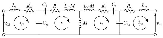
Figure 3.
Equivalent circuit of an LCC-compensated coupler.
With the aim of simplifying the mathematical modeling of the LCC-compensated system, only the mutual inductance between the coils and is considered. Thus, the remaining mutual inductances between the pairs of coils − , − and − are neglected. This assumption is valid in systems where there exists a proper isolation of the magnetic field in the coils and . For example, by reducing their leakage flux to a minimum with the use of a magnetic core and placing both coils sufficiently far from the magnetic coupler. Furthermore, this holds also true when and are integrated into the magnetic coupler so that the coupled flux in those coils is negligible, as in [44,45].
This time, the application of the superposition theorem results in the following system of differential equations for :
In turn, the case gives the second set of equations:
As stated previously in the mathematical analysis of the SS compensation, the subscripts and express the dependency of the currents on and in both systems of linear equations.
The translation of the expressions (12) and (13) into the frequency domain results in an equivalent set of equations that are noticeably more tedious and complex to solve than in the previous case. This time there are eight admittances to calculate that consist of high-order polynomials, either in the numerator or the denominator. It is convenient, therefore, to simplify the general equations by operating the IPT system at the resonance frequency and neglecting the parasitic resistances.
The tuning condition of the LCC topology is more complicated than in the case of the SS topology. This time, the system will be tuned at the resonant frequency () if the following expression is fulfilled [16]:
Under these assumptions, the currents at the and sides are given by [16]:
Thus, the apparent power at the input, , and output, , of the compensated coupler can be expressed as:
where, again, and are equal due to the ideal conditions under which they were derived.
It is apparent that the LCC compensation results in a more complex IPT system, which is a disadvantage when compared to the SS compensation. However, the following three specific issues make the LCC topology outperform its SS counterpart in an IPT system. First, when designing the magnetic coupler, its nominal operating current is established. Since and are independent of the load and the coupling coefficient, as stated in (16), a fully tuned LCC-compensated IPT system helps to keep both currents within a safe range [27,46]. Therefore, the LCC compensation provides a higher protection against saturation and deterioration of the magnetic coupler caused by excessively high currents. Moreover, it also prevents the saturation of magnetic couplers featuring ferrite cores, which are currently in widespread use in IPT prototypes designed for powering EVs.
The second significant advantage is the direct dependency of and with k, as follows from (15). As stated previously, if misalignment occurs or the air gap is increased, the value of k decreases. Consequently, both and decrease as well. The same occurs with the apparent power at both the inverter output and the rectifier input, as shown in (17) and (18).
Finally, it can be seen from (11) that the output power of an SS-compensated IPT system depends on and , on M and on . However, the output power of an LCC-compensated IPT system depends not only on those parameters but also on and , as stated previously in (18). This means that there exist two extra parameters in an LCC compensation that need to be designed, which is an interesting feature. The mutual inductance depends on both the misalignment and the air gap between coils, while the operating frequency range is determined by the standard SAE-J2954 [19]. Thus, both parameters cannot be used to adjust the power transferred in the design stage. With the double-sided LCC compensation, the added coils and can be used for this purpose. Therefore, the nominal voltages on the and sides can be determined from other constraints, such as the battery voltage.
3. Set-Up of the Simulation Model
The aim of this work is to evaluate the behavior of the SS and LCC topologies when the tolerance values are the only parameters that fluctuate. For this purpose, a sensitivity analysis was performed. The derivation of mathematical expressions results in a cumbersome work since the IPT system works out of the resonance condition. In addition, if the main assumptions are not fulfilled (e.g., negligible power losses and parasitic resistances), the simplified equations previously derived are no longer valid. To overcome these limitations, a simulation model was developed for each topology by using the Simscape Toolbox in Simulink. The same tools were used to run the models.
The selected variables to perform the analysis correspond to the RMS currents and the average power that flow through the compensation networks. For this purpose, the RMS values of the currents and (along with and for the LCC topology) were selected. Regarding the power estimations, the average active and apparent power at the input and output terminals of the compensated magnetic coupler were used. The average input and output powers were calculated using the first, third and fifth harmonic components throughout the analysis.
3.1. Design of the Compensation Parameters and Nominal Operating Point
In order to compare the SS and the LCC topologies, both simulated systems are tuned to work under the same resonant frequency and nominal apparent power. Furthermore, the coupling parameters , and k are kept constant so that both networks compensate an identical magnetic coupler. The same occurs with the DC voltages and , which are calculated by means of (1), (2) and (11), leading to the following expression:
For the sake of clarity, the values assigned to the parameters that remain unaltered in both compensated systems are shown in Table 1. The first (and easiest) system to tune corresponds to the SS topology. For this network, the capacitances are selected to make the system resonate at by means of the Equation (8):

Table 1.
Shared parameters between the SS and LCC compensations.
On the other hand, the tuning process for the LCC compensation follows the steps outlined in [27]. As a result, the following expressions for the values of the components are obtained:
The application of both design procedures results in the compensation parameters shown in Table 2. With the aim of simulating a realistic system, the parasitic resistances in each coil were included. In addition, the capacitances are accurate to a single decimal place, since the precision needed for a perfect tuning is hard to achieve in an experimental arrangement.
Table 2.
Unshared compensation parameters between the LCC and SS topologies
Through the use of Table 1 and Table 2, the nominal operating points (shown in Table 3) can be established. As can be seen, the apparent power achieved with both compensated systems differs slightly from the target value of 1 kW set for on Table 1. Moreover, the efficiency of the SS-compensated magnetic coupler is larger than the one obtained with the LCC compensation. According to [47], if , it follows that the efficiencies of both systems must be similar, provided the IPT systems are ideal. However, this does not hold exactly true in our case, owing to the influence of the parasitic resistances and the rounding of the compensation parameters. Thus, these two factors explain both the observed deviations from the expected and the lower efficiency of the LCC-compensated IPT system.
Table 3.
Nominal operating points for the simulated LCC- and SS-compensated systems
3.2. Assignment of Tolerances for the Multivariate Analysis
A key setting in the simulation models is the assignment of electrical component tolerances. In both studies, it is supposed that the values of all the components range from a minimum of 80% to a maximum of 120% of its nominal values. Hence, a tolerance range of % is set for each component.
In the multivariate analysis, the assigned tolerances follow a normal distribution characterized by a mean = 0 and a standard deviation = 6.6. This value for guarantees that % of the values of the ideal population are within the [, ] % range. Hence, limiting the minimum and maximum values of the generated sample to −20% and 20%, respectively, is a reasonable assumption. For each component, a different set of pseudo-random values was assigned by means of the MATLAB function randn with an initial sample size of 1500 values per component.
After simulating both systems, some of the obtained histograms had heavy tails. Consequently, the number of simulations was increased to 150,000 points for each topology. To illustrate this, Figure 4 shows a histogram and a scatter plot of the same variable for the two cases. Both histograms were normalized by using the probability density function (PDF) so that they can be compared avoiding the distortion caused by the sample size. The bigger data set gives a better match between the histogram and the fitted distribution, especially for the heavy tails. Moreover, the scatter plots show that the number of simulation points that fall near the 20% tolerance range is small for the data set of 1500 points. By increasing the number of simulations to 150,000, this is corrected.
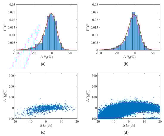
Figure 4.
Histograms and scatter plots used to illustrate the effect of augmenting the size of the data set. In subfigures (a,c) 1500 simulations were used, while subfigures (b,d) correspond to a data set of 150,000 points.
The histograms obtained for the tolerances assigned in the SS-compensated system take the form shown in Figure 5. Here, the number of occurrences (hereafter called frequency) is shown and the fitted normal distributions are superimposed. In order to calculate the bin width of each histogram, the Sturges’ rule is applied to a specified range. Taking as the range width, the bin width of the histogram can be calculated as [48]:
where n corresponds to the number of observations located within the selected range.
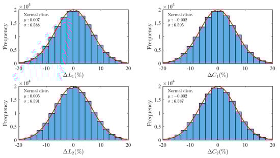
Figure 5.
Histograms of the tolerances assigned to each parameter during the Monte-Carlo simulation of the SS-compensated system.
For the histograms shown in Figure 5, the [, 20] % range was selected. As a result, a bin width of % is obtained for the 150,000 simulations in the sample. The use of the Freedman-Diaconis rule was also evaluated. However, the resulting bin widths were excessively narrow, not only for the above-mentioned histograms but for others used later in this work.
As can be seen, the and values obtained for each case in Figure 5 are close to their respective initial settings. In addition, the histograms follow appropriately a normal distribution, hence the population is large enough. Moreover, it can be seen from and that each population slightly differs from the others. This procedure was also followed for the LCC compensation parameters and the results are very similar. Consequently (and for the sake of brevity), their histograms are not shown.
4. Analysis of the Monte-Carlo Simulations
The multivariate analysis focuses on the comparison between the SS and the LCC compensations when the component values vary simultaneously. For this purpose, two complementary approaches are applied.
First, the evaluation of the trends observed for the currents, the active and the apparent power (hereafter defined together as variables) is performed through the use of normalized histograms. The normalization used in this work corresponds to an estimate of the PDF of the sample. To calculate the bin width, the range where the fitted PDF cannot be ignored is selected for each variable. The empirical PDFs are fitted using stable distributions, unless otherwise indicated. This distribution is appropriate for the analysis since the deviations from the nominal operating point are caused by the normally distributed variations of the tolerances. The distribution fitting of the histograms was carried out by using the MATLAB function fitdist.
Secondly, scatter plots are represented. The primary purpose of this approach is to find out whether or not there exist a strong correlation between the tolerances of each component and any of the variables. If such correlations exist, the equation for a straight line is obtained along with the Pearson and the determination (or R-squared, ) coefficients. The Pearson correlation coefficient helps to determine how accurate the hypothesis of a linear dependency between both variables is. On the other hand, the accounts for the percentage of the variation of the sample that can be explained by the model.
With the aim of avoiding the use of units, both the variables and component quantities are expressed as deviations from its nominal values. In doing so, the analyzed data do not correspond to absolute values but to relative increments instead, avoiding misinterpretations derived from scale effects.
4.1. SS-Compensated IPT System
The histograms that result from the simulation of the SS-compensated system are shown in Figure 6. The x-axis stretches from % to 70% for all the variables under consideration because most of the simulated data fit within that range in both topologies. However, a few fall beyond these limits. The IPT system is compensated with resonant networks, thus it is inherently sensitive to the deviations of the components. Hence, the operation off resonance may result in either a significant increase or decrease of the measured variables. For example, the maximum deviations observed during the Monte-Carlo simulations correspond to % and % for the SS topology. Regarding the LCC compensation, % and % are the maximum values observed. These deviations are in agreement with those reported in [16], where the output power vary from 0 W to more than 11.5 kW for a 5.7 kW LCC-compensated IPT system in a [, 10] % tolerance range. For the sake of accuracy, it should be pointed out that none of the data points that fall outside the chosen range are disregarded in the computational work. Their exclusion is only effective in the visualization of the histograms.
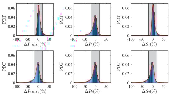
Figure 6.
Normalized histograms of the measurements for the SS compensation.
For a better understanding of the distribution profiles obtained from the simulations, the range [, 20] %, is shadowed in the histograms. It corresponds to the boundaries previously set for the variation of the components. Please note that outside these boundaries, the and sides respond quite differently. On the side, the simulated data for and largely exceed the 20% upper boundary, resulting in positively skewed distribution profiles in both cases. On the contrary, both and on the side appear well below the % lower boundary. A similar divergent trend is observed when comparing , which has certain deviations near %, with , where most of the simulated data exhibit positive percentage deviations. The observed distribution profiles are in agreement with the increase in reactive power produced by the detuned networks. Thus, the power transfer capability of the IPT system is reduced. For this reason, both the RMS current , the active power and the apparent power on the side decrease as a consequence of the corresponding fall undergone by .
If the area of the bars covered by the [, 20] % range is compared with the whole surface represented in the histogram, the empirical probability for that particular range is obtained. This statistical parameter is shown in Table 4. As can be seen, the empirical probabilities for and are remarkably larger. This is entirely consistent with the distribution profiles observed in the histograms, where a relevant percentage of the simulations are located near the nominal operating point for and .
Table 4.
Estimated empirical probability of the variables under study for the SS-compensated system
The x-axis in the scatter plots ranges from % to 20% while the y-axis is set up so that all the simulated data points are included. For the sake of clarity, all the graphics obtained for each pair component-variable are shown in Appendix A. Only one dispersion graph per variable is shown in Figure 7, except for the efficiency. As can be seen, there is not a strong correlation for most of the represented variables. The lack of such correlations in the multivariate analysis is not surprising since the simultaneous variation of two or more components influence the samples involved in each variable. However, this result is not necessarily expected in the univariate case, where strong correlations may occur in certain cases. To illustrate this, Figure 8 shows the variations of , and when all parameters are kept constant except . For this analysis, the tolerances vary from −20% to 20% in steps of 0.4%. As there is no other variation that affects the sample in neither of the three cases, the correlations between those variables and can be clearly seen. However, such correlations are not so evident in the multivariate plots shown in Figure 7.
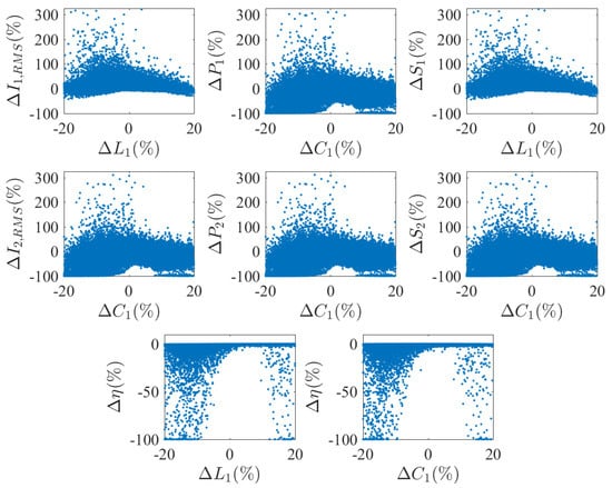
Figure 7.
Selection of scatter plots for the variables under study in the SS-compensated system when all the compensation components vary simultaneously within their respective tolerance ranges. Each plot represents the degree of correlation found between a simulated variable and a single component.
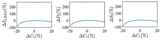
Figure 8.
Variations in , and when is the only parameter that varies within its tolerance range.
By inspecting the dispersion graphs for shown in Figure 7, it is apparent that small tolerances may lead to a reduction in the variations observed. However, those tolerances must be significantly small to keep such deviations within reasonable limits. Unfortunately, this is difficult to achieve for the coupler coils, since the tolerance range of commercial coils is usually large.
On the other hand, it should be noted that the scatter plots for and and their corresponding correlations are quite similar to each other. However, owing to the increase undergone by the reactive power under detuning conditions, this does not hold true for and .
4.2. LCC-Compensated System
The histograms for the variables of the LCC-compensated system are shown in Figure 9. Here, the x- and y-axes boundaries are the same as in the SS compensation analysis so that the distribution profiles obtained in both cases can be compared without distortion. Again, some data points are not represented in the histograms despite being considered in the fitting.
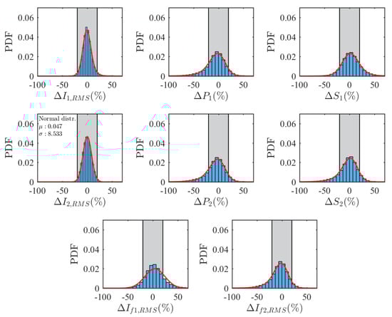
Figure 9.
Normalized histograms of the measurements for the LCC compensation.
When comparing the histograms shown in Figure 9 with those in Figure 6, it can be concluded that the distribution profiles of the LCC network are more symmetrical. Aiming at a better interpretation of these distribution profiles, the obtained values for the empirical probabilities are collected in Table 5. In general terms, a decrease in the empirical probabilities is observed except for the RMS values of the currents and . In fact, when the empirical probabilities of both currents are calculated within the broader range of [, 30] %, their values increase to nearly 100% for the LCC compensation. The resulting probabilities are 99.20% for and 99.95% for , whereas in the case of the SS topology the calculations result in 96.99% and 90.25%, respectively. This means that despite the higher dispersion observed, the LCC compensation maintains the RMS currents at both sides of the magnetic coupler nearer its nominal values.
Table 5.
Estimated empirical probability of the variables under study for the LCC-compensated system
Please note that in this case the resulting distribution profiles for the active and apparent power are not so different from each other as they turn out to be with the SS compensation. The operation of the IPT system off resonance necessarily increases the reactive power regardless of the compensation network used. However, it is apparent from the power histograms that the power transfer capability is compromised to a lesser extent if an LCC instead of an SS compensation is used. This is consistent with the conclusions drawn in [19].
The entire set of scatter plots obtained for the LCC-compensated system are collected in Appendix B, whereas one dispersion graph per variable is shown in Figure 10. As can be seen, there is a noticeable correlation between the pair and also between the pair . Consequently, the variations on and can be reduced simply by selecting capacitors and characterized by tolerance figures as small as possible. To illustrate this, a comparative example is shown in Table 6. It compares the maximum deviations found in the entire data set with those obtained for a subset where the tolerance range for and is [, 5] %. From the 150,000 points in the sample, 44,777 points meet this requirement.
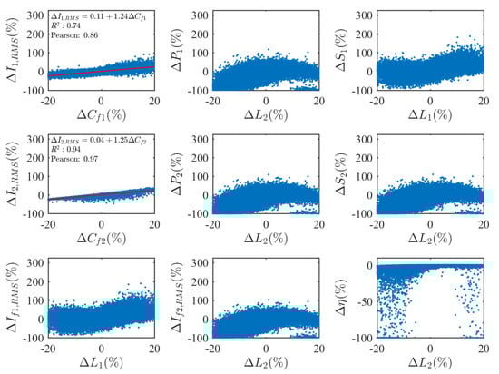
Figure 10.
Selection of scatter plots for the variables under study in the LCC-compensated system when all the compensation components vary simultaneously within their respective tolerance ranges. Each plot represents the degree of correlation found between a simulated variable and a single component.
Table 6.
Maximum deviations obtained for and under different tolerance values assigned to and .
Upon comparing the results, it is apparent that a significant reduction in the tolerance interval contributes to narrow down the shifts from their nominal values undergone by the currents. In particular, it helps to prevent significant increases in both currents. Obviously, the number of possible combinations with non-zero tolerances in a real system is virtually infinite. Thus, the deviations shown in Table 6 must be taken with caution. Nevertheless, this is an interesting result of practical interest in the design of IPT systems. The adjustment of the tolerances of the capacitors and gives a way of controlling, at least to a certain extent, the potentially large increments in and .
5. Conclusions
In this work, the influence that the tolerances of the compensation components have on both an SS- and a double-sided LCC-compensated IPT system was investigated. For this purpose, the variations in the currents, the power transferred, and the efficiency were evaluated for both topologies. The main characteristics of each compensation topology are first highlighted for the case of a fully tuned system through a mathematical analysis. Secondly, the expected behavior of the two detuned networks is compared through a Monte-Carlo analysis.
The mathematical analysis shows that both topologies have a current-source behavior at the output of the side for a fully tuned system, provided the RMS voltage at the VSI output is constant. Under these conditions, the lower cost and reduced complexity of the SS-compensated IPT system are valuable advantages. However, the output power is inversely related with the coupling coefficient k in the SS topology, which may result in an unsafe operation when misalignment occurs. This drawback can be solved by using an LCC compensation instead, for which output power and k are directly proportional. Moreover, the RMS currents on both sides of the magnetic coupler remain constant against variations in either the load or k. This fact makes the LCC network stand out as the preferred choice when a high uncertainty in any of the two parameters is expected.
The Monte-Carlo analysis reveals that the SS compensation leads to an overall smaller deviation from its nominal operating point against the variation of the compensation components. However, this does not hold true for the currents through the coils of the magnetic coupler. For and , the LCC topology shows a better capability to maintain both currents within the [, 20] % range. Moreover, the LCC-compensated IPT system shows a smaller increase in the reactive power. Thus, a higher power transfer capability under detuning conditions is obtained. In addition, correlations between and and also between and arose from the scatter plots corresponding to the LCC compensation. Hence, the increase in both currents can be limited, at least to a certain extent, simply by selecting capacitors with low tolerance values for and . This is arguably a result of practical interest in the design of IPT systems.
In conclusion, despite its higher complexity and cost, the LCC compensation guarantees a safer operation when there is a high degree of uncertainty in k. In addition, it has a higher power transfer capability and provides a tighter control of the RMS currents on both coils in the magnetic coupler. Nevertheless, the SS network is still an appropriate choice for those IPT systems where size and weight must be optimized.
Author Contributions
Conceptualization, F.J.L.-A. and J.V.; methodology, F.J.L.-A. and P.R.-S.; software, F.J.L.-A.; validation, J.V., P.R.-S. and A.P.T.; formal analysis, F.J.L.-A., J.V. and E.J.M.-M.; investigation, J.V. and P.R.-S.; resources, P.R.-S. and J.V.; writing—original draft preparation, F.J.L.-A. and J.V.; writing—review and editing, F.J.L.-A., J.V. and P.R.-S.; visualization, F.J.L.-A. and E.J.M.-M.; supervision, P.R.-S. and A.P.T.; project administration, P.R.-S.; funding acquisition, P.R.-S. All authors have read and agreed to the published version of the manuscript.
Funding
This research received no external funding.
Conflicts of Interest
The authors declare no conflict of interest. The funders had no role in the design of the study; in the collection, analyses, or interpretation of data; in the writing of the manuscript, or in the decision to publish the results.
Abbreviations
The following abbreviations are used in this manuscript:
| EV | Electric Vehicle |
| WPT | Wireless Power Transfer |
| Ground Assembly | |
| Vehicle Assembly | |
| CPT | Capacitive Power Transfer |
| IPT | Inductive Power Transfer |
| G2V | Grid-to-Vehicle |
| SS | Series-Series |
| k | Coupling coefficient |
| PP | Parallel-Parallel |
| LCC | Inductor-Capacitor-Capacitor |
| VSI | Voltage Source Inverter |
| Probability Density Function |
Appendix A. Scatter Plots for the SS-Compensated System

Figure A1.
Scatter plots showing the variation of for an SS-compensated system.

Figure A2.
Scatter plots showing the variation of for an SS-compensated system.

Figure A3.
Scatter plots showing the variation of for an SS-compensated system.

Figure A4.
Scatter plots showing the variation of for an SS-compensated system.

Figure A5.
Scatter plots showing the variation of for an SS-compensated system.

Figure A6.
Scatter plots showing the variation of for an SS-compensated system.

Figure A7.
Scatter plots showing the variation of for an SS-compensated system.
Appendix B. Scatter Plots for the LCC-Compensated System

Figure A8.
Scatter plots showing the variation of for an LCC-compensated system.

Figure A9.
Scatter plots showing the variation of for an LCC-compensated system.

Figure A10.
Scatter plots showing the variation of for an LCC-compensated system.

Figure A11.
Scatter plots showing the variation of for an LCC-compensated system.

Figure A12.
Scatter plots showing the variation of for an LCC-compensated system.

Figure A13.
Scatter plots showing the variation of for an LCC-compensated system.

Figure A14.
Scatter plots showing the variation of for an LCC-compensated system.

Figure A15.
Scatter plots showing the variation of for an LCC-compensated system.

Figure A16.
Scatter plots showing the variation of for an LCC-compensated system.
References
- Standard, S. Wireless Power Transfer for Light-Duty Plug-In/Electric Vehicles and Alignment Methodology. In SAE J2954 TIR; SAE: Warrendale, PA, USA, 2019. [Google Scholar] [CrossRef]
- Al-Saadi, M.; Al-Gizi, A.; Ahmed, S.; Al-Chlaihawi, S.; Craciunescu, A. Analysis of Charge Plate Configurations in Unipolar Capacitive Power Transfer System for the Electric Vehicles Batteries Charging. Procedia Manuf. 2019, 32, 418–425. [Google Scholar] [CrossRef]
- Zhu, Q.; Zou, L.J.; Su, M.; Hu, A.P. Four-plate capacitive power transfer system with different grounding connections. Int. J. Electr. Power Energy Syst. 2020, 115, 105494. [Google Scholar] [CrossRef]
- Lu, F.; Zhang, H.; Hofmann, H.; Mi, C.C. An Inductive and Capacitive Combined Wireless Power Transfer System WithLC-Compensated Topology. IEEE Trans. Power Electron. 2016, 31, 8471–8482. [Google Scholar] [CrossRef]
- Regensburger, B.; Kumar, A.; Sinha, S.; Doubleday, K.; Pervaiz, S.; Popovic, Z.; Afridi, K. High-performance large air-gap capacitive wireless power transfer system for electric vehicle charging. In Proceedings of the 2017 IEEE Transportation Electrification Conference and Expo (ITEC), Chicago, IL, USA, 22–24 June 2017; pp. 638–643. [Google Scholar] [CrossRef]
- Bosshard, R.; Iruretagoyena, U.; Kolar, J.W. Comprehensive Evaluation of Rectangular and Double-D Coil Geometry for 50 kW/85 kHz IPT System. IEEE J. Emerg. Sel. Top. Power Electron. 2016, 4, 1406–1415. [Google Scholar] [CrossRef]
- Zhang, W.; White, J.C.; Abraham, A.M.; Mi, C.C. Loosely Coupled Transformer Structure and Interoperability Study for EV Wireless Charging Systems. IEEE Trans. Power Electron. 2015, 30, 6356–6367. [Google Scholar] [CrossRef]
- Deng, J.; Li, W.; Nguyen, T.D.; Li, S.; Mi, C.C. Compact and Efficient Bipolar Coupler for Wireless Power Chargers: Design and Analysis. IEEE Trans. Power Electron. 2015, 30, 6130–6140. [Google Scholar] [CrossRef]
- Li, Y.; Zhao, J.; Yang, Q.; Liu, L.; Ma, J.; Zhang, X. A Novel Coil With High Misalignment Tolerance for Wireless Power Transfer. IEEE Trans. Magn. 2019, 55, 1–4. [Google Scholar] [CrossRef]
- Olukotun, B.; Partridge, J.; Bucknall, R. Finite Element Modeling and Analysis of High Power, Low-loss Flux-Pipe Resonant Coils for Static Bidirectional Wireless Power Transfer. Energies 2019, 12, 3534. [Google Scholar] [CrossRef]
- Sis, S.A.; Orta, E. A Cross-Shape Coil Structure for Use in Wireless Power Applications. Energies 2018, 11, 1094. [Google Scholar] [CrossRef]
- Castillo-Zamora, I.U.; Huynh, P.S.; Vincent, D.; Perez-Pinal, F.J.; Rodriguez-Licea, M.A.; Williamson, S. Hexagonal Geometry Coil for a WPT High Power Fast Charging Application. IEEE Trans. Transp. Electrif. 2019, 5, 946–956. [Google Scholar] [CrossRef]
- Kalwar, K.A.; Mekhilef, S.; Seyedmahmoudian, M.; Horan, B. Coil Design for High Misalignment Tolerant Inductive Power Transfer System for EV Charging. Energies 2016, 9, 937. [Google Scholar] [CrossRef]
- Lu, F.; Zhang, H.; Mi, C. A Review on the Recent Development of Capacitive Wireless Power Transfer Technology. Energies 2017, 10, 1752. [Google Scholar] [CrossRef]
- Yusop, Y.; Saat, S.; Husin, H.; Nguang, S.K.; Hindustan, I. Analysis of Class-E LC Capacitive Power Transfer System. Energy Procedia 2016, 100, 287–290. [Google Scholar] [CrossRef]
- Lu, F.; Zhang, H.; Hofmann, H.; Mi, C. A Double-SidedLCLC-Compensated Capacitive Power Transfer System for Electric Vehicle Charging. IEEE Trans. Power Electron. 2015, 30, 6011–6014. [Google Scholar] [CrossRef]
- Machura, P.; Li, Q. A critical review on wireless charging for electric vehicles. Renew. Sustain. Energy Rev. 2019, 104, 209–234. [Google Scholar] [CrossRef]
- Shevchenko, V.; Husev, O.; Strzelecki, R.; Pakhaliuk, B.; Poliakov, N.; Strzelecka, N. Compensation Topologies in IPT Systems: Standards, Requirements, Classification, Analysis, Comparison and Application. IEEE Access 2019, 7, 120559–120580. [Google Scholar] [CrossRef]
- Li, W.; Zhao, H.; Deng, J.; Li, S.; Mi, C.C. Comparison Study on SS and Double-Sided LCC Compensation Topologies for EV/PHEV Wireless Chargers. IEEE Trans. Veh. Technol. 2016, 65, 4429–4439. [Google Scholar] [CrossRef]
- Villa, J.L.; Sallan, J.; Sanz Osorio, J.F.; Llombart, A. High-Misalignment Tolerant Compensation Topology For ICPT Systems. IEEE Trans. Ind. Electron. 2012, 59, 945–951. [Google Scholar] [CrossRef]
- Samanta, S.; Rathore, A.K. A New Current-Fed CLC Transmitter and LC Receiver Topology for Inductive Wireless Power Transfer Application: Analysis, Design, and Experimental Results. IEEE Trans. Transp. Electrif. 2015, 1, 357–368. [Google Scholar] [CrossRef]
- Hou, J.; Chen, Q.; Wong, S.; Tse, C.K.; Ruan, X. Analysis and Control of Series/Series-Parallel Compensated Resonant Converter for Contactless Power Transfer. IEEE J. Emerg. Sel. Top. Power Electron. 2015, 3, 124–136. [Google Scholar] [CrossRef]
- Keeling, N.A.; Covic, G.A.; Boys, J.T. A Unity-Power-Factor IPT Pickup for High-Power Applications. IEEE Trans. Ind. Electron. 2010, 57, 744–751. [Google Scholar] [CrossRef]
- Madawala, U.K.; Thrimawithana, D.J. A Bidirectional Inductive Power Interface for Electric Vehicles in V2G Systems. IEEE Trans. Ind. Electron. 2011, 58, 4789–4796. [Google Scholar] [CrossRef]
- Xia, C.; Chen, R.; Liu, Y.; Chen, G.; Wu, X. LCL/LCC resonant topology of WPT system for constant current, stable frequency and high-quality power transmission. In Proceedings of the 2016 IEEE PELS Workshop on Emerging Technologies: Wireless Power Transfer (WoW), Knoxville, TN, USA, 4–6 October 2016; pp. 110–113. [Google Scholar] [CrossRef]
- Thrimawithana, D.J.; Madawala, U.K. A Generalized Steady-State Model for Bidirectional IPT Systems. IEEE Trans. Power Electron. 2013, 28, 4681–4689. [Google Scholar] [CrossRef]
- Li, S.; Li, W.; Deng, J.; Nguyen, T.D.; Mi, C.C. A Double-Sided LCC Compensation Network and Its Tuning Method for Wireless Power Transfer. IEEE Trans. Veh. Technol. 2015, 64, 2261–2273. [Google Scholar] [CrossRef]
- Varikkottil, S.; Febin Daya, J.L. High-gain LCL architecture based IPT system for wireless charging of EV. IET Power Electron. 2019, 12, 195–203. [Google Scholar] [CrossRef]
- Yan, Z.; Zhang, Y.; Song, B.; Zhang, K.; Kan, T.; Mi, C. An LCC-P Compensated Wireless Power Transfer System with a Constant Current Output and Reduced Receiver Size. Energies 2019, 12, 172. [Google Scholar] [CrossRef]
- Chen, Y.; Zhang, H.; Park, S.J.; Kim, D.H. A Comparative Study of S-S and LCCL-S Compensation Topologies in Inductive Power Transfer Systems for Electric Vehicles. Energies 2019, 12, 1913. [Google Scholar] [CrossRef]
- Ann, S.; Lee, W.Y.; Choe, G.Y.; Lee, B.K. Integrated Control Strategy for Inductive Power Transfer Systems with Primary-Side LCC Network for Load-Average Efficiency Improvement. Energies 2019, 12, 312. [Google Scholar] [CrossRef]
- Geng, Y.; Li, B.; Yang, Z.; Lin, F.; Sun, H. A High Efficiency Charging Strategy for a Supercapacitor Using a Wireless Power Transfer System Based on Inductor/Capacitor/Capacitor (LCC) Compensation Topology. Energies 2017, 10, 135. [Google Scholar] [CrossRef]
- Ramezani, A.; Farhangi, S.; Iman-Eini, H.; Farhangi, B.; Rahimi, R.; Moradi, G.R. Optimized LCC-Series Compensated Resonant Network for Stationary Wireless EV Chargers. IEEE Trans. Ind. Electron. 2019, 66, 2756–2765. [Google Scholar] [CrossRef]
- Zhang, Y.; Yan, Z.; Kan, T.; Liu, Y.; Mi, C.C. Modelling and analysis of the distortion of strongly-coupled wireless power transfer systems with SS and LCC–LCC compensations. IET Power Electron. 2019, 12, 1321–1328. [Google Scholar] [CrossRef]
- Mohamed, A.A.S.; Berzoy, A.; de Almeida, F.G.N.; Mohammed, O. Modeling and Assessment Analysis of Various Compensation Topologies in Bidirectional IWPT System for EV Applications. IEEE Trans. Ind. Appl. 2017, 53, 4973–4984. [Google Scholar] [CrossRef]
- Lu, F.; Hofmann, H.; Deng, J.; Mi, C. Output power and efficiency sensitivity to circuit parameter variations in double-sided LCC-compensated wireless power transfer system. In Proceedings of the 2015 IEEE Applied Power Electronics Conference and Exposition (APEC), Charlotte, NC, USA, 15–19 March 2015; pp. 597–601. [Google Scholar] [CrossRef]
- Lu, S.; Deng, X.; Shu, W.; Wei, X.; Li, S. A New ZVS Tuning Method for Double-Sided LCC Compensated Wireless Power Transfer System. Energies 2018, 11, 307. [Google Scholar] [CrossRef]
- Hart, D.W. Power Electronics; Tata McGraw-Hill Education: New York, NY, USA, 2011. [Google Scholar]
- Li, Z.; Zhu, C.; Jiang, J.; Song, K.; Wei, G. A 3-kW Wireless Power Transfer System for Sightseeing Car Supercapacitor Charge. IEEE Trans. Power Electron. 2017, 32, 3301–3316. [Google Scholar] [CrossRef]
- Vázquez, J.; Roncero-Sánchez, P.; Parreño Torres, A. Simulation Model of a 2-kW IPT Charger with Phase-Shift Control: Validation through the Tuning of the Coupling Factor. Electronics 2018, 7, 255. [Google Scholar] [CrossRef]
- Dehui, W.; Qisheng, S.; Xiaohong, W.; Fan, Y. Analytical model of mutual coupling between rectangular spiral coils with lateral misalignment for wireless power applications. IET Power Electron. 2018, 11, 781–786. [Google Scholar] [CrossRef]
- López-Alcolea, F.J.; del Real, J.V.; Roncero-Sánchez, P.; Torres, A.P. Modeling of a Magnetic Coupler Based on Single- and Double-Layered Rectangular Planar Coils With In-Plane Misalignment for Wireless Power Transfer. IEEE Trans. Power Electron. 2020, 35, 5102–5121. [Google Scholar] [CrossRef]
- Del Toro García, X.; Vázquez, J.; Roncero-Sánchez, P. Design, implementation issues and performance of an inductive power transfer system for electric vehicle chargers with series–series compensation. IET Power Electron. 2015, 8, 1920–1930. [Google Scholar] [CrossRef]
- Kan, T.; Nguyen, T.; White, J.C.; Malhan, R.K.; Mi, C.C. A New Integration Method for an Electric Vehicle Wireless Charging System Using LCC Compensation Topology: Analysis and Design. IEEE Trans. Power Electron. 2017, 32, 1638–1650. [Google Scholar] [CrossRef]
- Kan, T.; Lu, F.; Nguyen, T.; Mercier, P.P.; Mi, C.C. Integrated Coil Design for EV Wireless Charging Systems Using LCC Compensation Topology. IEEE Trans. Power Electron. 2018, 33, 9231–9241. [Google Scholar] [CrossRef]
- Liu, C.; Ge, S.; Guo, Y.; Li, H.; Cai, G. Double-LCL resonant compensation network for electric vehicles wireless power transfer: Experimental study and analysis. IET Power Electron. 2016, 9, 2262–2270. [Google Scholar] [CrossRef]
- Liu, X.; Clare, L.; Yuan, X.; Wang, C.; Liu, J. A Design Method for Making an LCC Compensation Two-Coil Wireless Power Transfer System More Energy Efficient Than an SS Counterpart. Energies 2017, 10, 1346. [Google Scholar] [CrossRef]
- Scott, D.W. Multivariate Density Estimation: Theory, Practice, and Visualization; John Wiley & Sons: Hoboken, NJ, USA, 2015. [Google Scholar]
© 2020 by the authors. Licensee MDPI, Basel, Switzerland. This article is an open access article distributed under the terms and conditions of the Creative Commons Attribution (CC BY) license (http://creativecommons.org/licenses/by/4.0/).