Influence Analysis and Stepwise Regression of Coal Mechanical Parameters on Uniaxial Compressive Strength Based on Orthogonal Testing Method

Abstract

Uniaxial compressive strength (UCS) and peak strain (PS) are essential indices for studying the mechanical properties of coal and rock masses, and they are closely related to mechanical parameters such as the elastic modulus (E), Poisson’s ratio (υ), cohesion (C) and internal friction angle (Φ) of coal and rock masses. This study took the No. 2-1 coal seam of Zhaogu No. 2 Mine, in Henan Province, China, as the research object. An RMT-150B servo testing machine was used to test all mechanical parameters, including the E, υ, C and Φ of coal and rock masses. Based on the principle of orthogonal testing, Three Dimensions Fast Lagrangian Analysis of Continua (FLAC3D) was used to select E, υ, C, Φ, tensile strength (R_m) and dilation angle (Ψ) as initial participation factors. Using these six parameters and a five-level combination scheme (L₂₅ (5⁶)), the influence of coal mechanical parameters on UCS and PS was investigated, using the software SPSS for stepwise regression analysis, and a uniaxial pressure-resistant regression prediction equation was established. The research showed that, under uniaxial compression conditions, the main parameters controlling UCS of coal masses are C and Φ; conversely, the main parameters controlling PS are E and C. UCS and PS exhibit significant linear relationships with these main controlling parameters. Here, a stepwise regression prediction equation was established through reliability verification analysis using the main controlling parameters. This prediction method produces very small errors and a good degree of fit, thus allowing the rapid prediction of UCS. The precision of the stepwise regression model depends on the number of test samples, which can be increased in the later stages of a design project to further improve the precision of the projection model.

1. Introduction

UCS and PS are significant indices in the study of the mechanical properties of coal and rock masses and have been used widely in the design of underground mining [1,2,3,4,5]. UCS and PS are closely related to other mechanical parameters of coal and rock masses, including E, υ, C, Φ, R_m and Ψ. The mechanical parameters of coal masses exhibit considerable spatial variability owing to the effects of coal-forming geological conditions and structural geology. Diversity in these mechanical parameters leads to large variation in UCS and PS, which in turn has a considerable effect on the mechanical response characteristics of coal, including rock burst strength and the degree of deformation of the rock mass surrounding roadways [6,7,8,9,10,11,12]. Thus, the influence of mechanical parameters on UCS and PS has been researched and the main parameters controlling the characteristics of coal mass strength have been determined; accordingly, the rapid and accurate prediction of UCS of coal masses based on mechanical parameters has been made possible. Such knowledge is of critical importance for the prevention and control of rock failure.

While exploring the relationship between UCS, PS and mechanical parameters and investigating the prediction of UCS, predecessors have carried out extensive research based on accumulated engineering data [13,14,15,16,17,18,19,20]. For instance, He et al. [21] used the fuzzy positive correlation between UCS and E to establish a correlation between UCS and E for sedimentary rocks with 10 different types of structure. Yang et al. [22] used the SPSS 19.0 statistical software to establish six separate mathematical regression models, taking UCS as the dependent variable and E as the independent variable; they also obtained a variable quadratic nonlinear regression prediction equation. Mahdi et al. [23] indirectly estimated the reliability of predicting UCS, Brazilian tensile strength (BTS) and E of marlstone using a single compressive strength method. Considering the randomness and fuzziness inherent in the determination of rock UCS, Qi et al. [24] obtained 88 groups of test data through uniaxial compression experiments, taking UCS as the dependent variable and E and natural density as independent variables, and established a multiple linear regression model. Lin and Xu [25] used linear function, quadratic function and power function regression models to fit the relationship between UCS and E for coal measure strata based on differences in lithology, taking E as the independent variable and UCS as the dependent variable. Hu et al. [26] established a multiple linear regression prediction model for the UCS and E values of the Pengguan complex, adopting the measured UCS and E values as dependent variables and rock block density, Schmidt rebound hardness and the geological strength index as independent variables. Piotr et al. [27] measured three types of Young’s modulus according to International Society for Rock Mechanics (ISRM) methods in an indoor uniaxial compression experiment, obtained correlation expressions of the tangent modulus, secant modulus and average modulus with UCS and evaluated the consistency of three UCS–E mathematical models.

Most previous studies have simply analyzed the correlation between single mechanical parameters and UCS, and little attention has been paid to the comprehensive correlation among multiple mechanical parameters, UCS and PS. Additionally, predictions of the UCS of coal seams have rarely been reported. Accordingly, this study took the No. 2-1 coal seam of Zhaogu No. 2 Mine in Henan Province as the case study. An RMT-150B servo testing machine was used for the uniaxial compression test, Brazilian splitting test and triaxial test of coal samples to determine the mechanical parameters. Based on orthogonal experiment, six mechanical parameters were selected: E, υ, C, Φ, R_m and Ψ. Using these six factors and a five-level combination scheme (L₂₅ (5⁶)), the influence of coal mechanical parameters on the uniaxial compression test and peak strain was investigated, with FLAC3D finite difference software used to simulate each scheme and determine the main control factors affecting the UCS and PS. SPSS software was used to establish a stepwise regression model for predicting UCS to obtain a regression equation for predicting UCS when adopting the main control factors and verify the reliability. To realize the above research contents, mechanical parameters such as UCS, C, Φ and υ of coal samples were obtained through mechanical tests, so as to facilitate the orthogonal numerical simulation test. Then, the FLAC3D simulation software was used to establish the numerical model. Based on the study of the mesh generation, constitutive model and loading rate, the numerical simulation conditions for the mechanical properties of coal samples were established. At the same time, according to the principle of orthogonal experiment, the horizontal spacing of six factors and five levels was determined, the horizontal parameters were listed, and the numerical simulation scheme of orthogonal experiment was determined. Finally, according to the numerical simulation results, the influence degree of each mechanical parameter on peak strength and peak strain was analyzed, in order to determine the main control factors. The stepwise regression prediction model of UCS was established by SPSS software, and the reliability of the model was verified. The specific technical roadmap is shown in Figure 1.

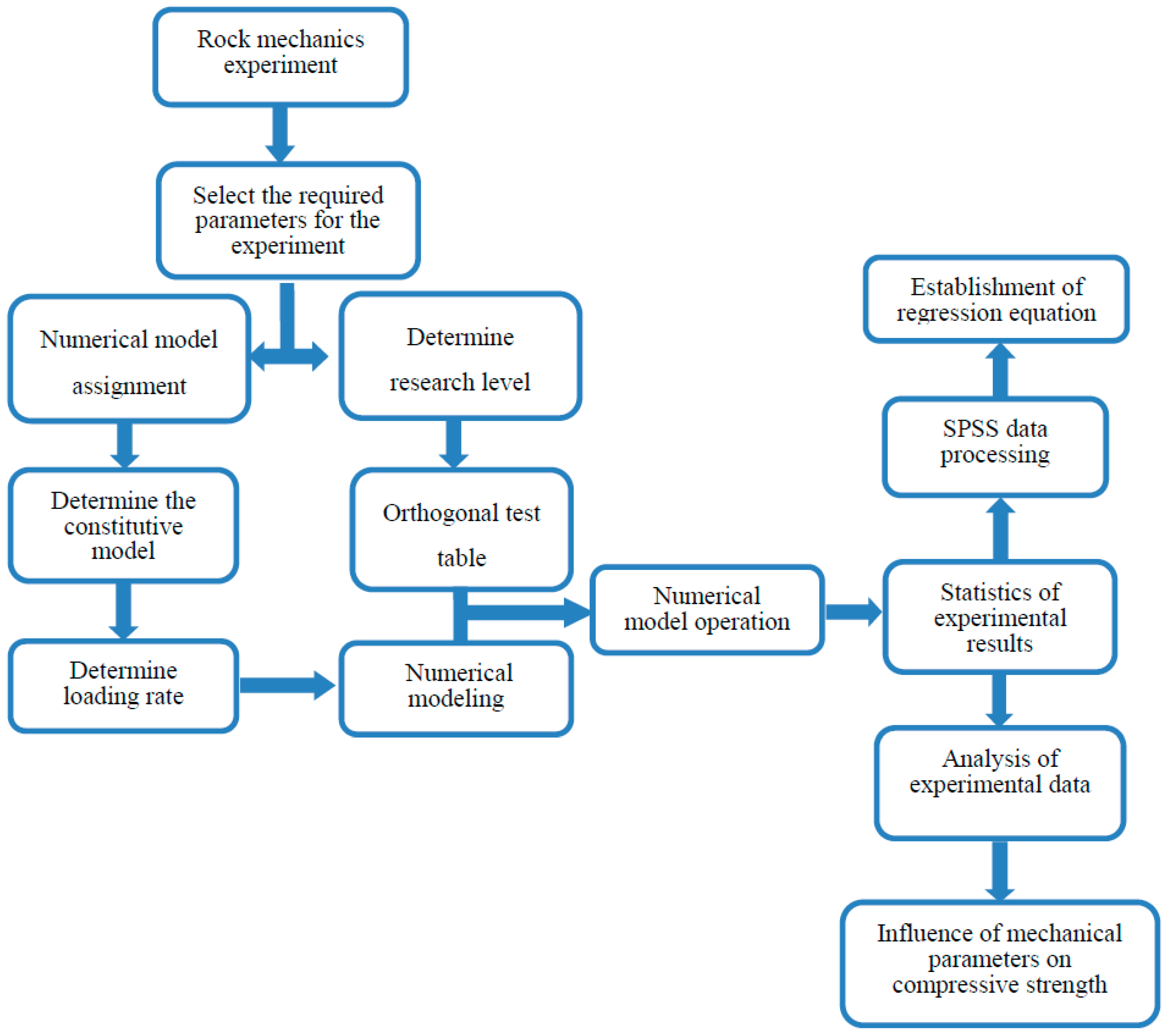
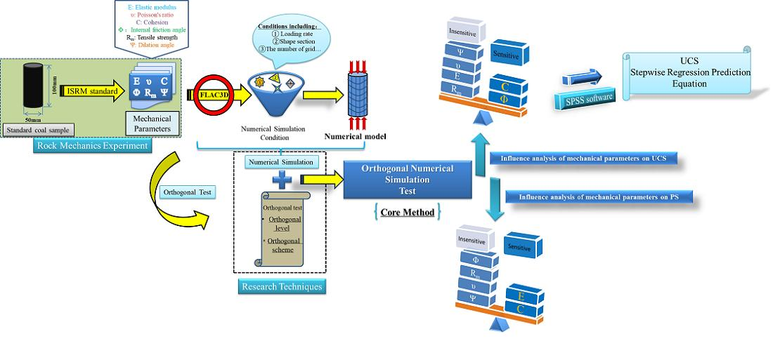
2. Orthogonal Numerical Simulation Experiments

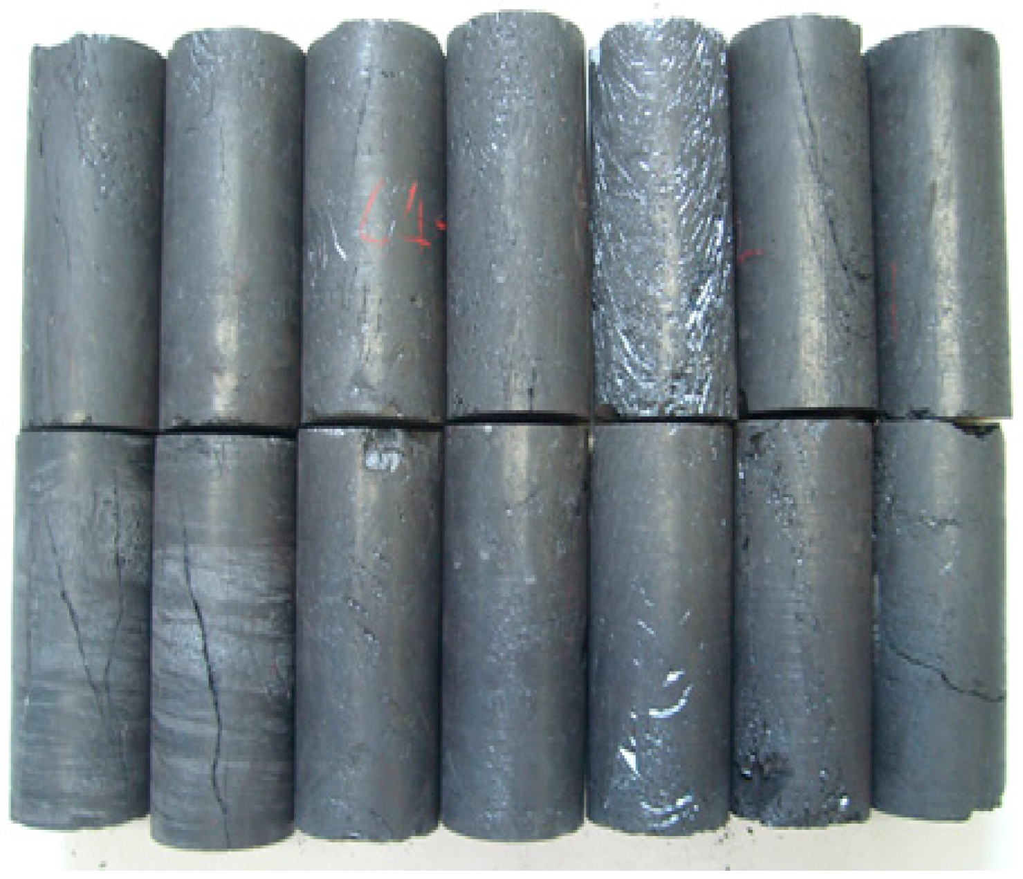
2.1. Production of Coal Samples

The main coal seam of Zhaogu No. 2 mine is the Permian Shanxi formation No. 2-1 coal seam. The dip angle of the coal seam is between 2° and 6°, and the average thickness is 6.16 m; this forms a thick, stable and near-horizontal coal seam. The coal is high quality anthracite with medium ash, low sulfur, high calorific value and high ash melting point. The coal seam is simple in structure, being mainly composed of lump coal and partially filled with calcite, some of which contains parting and mudstone interlayers. The coal seam is characterized by the development of endogenous fissures and the high strength of its lump coal. The average natural apparent density of the coal seam is 1435 kg/m³.

To ensure the reliability of the test data, four sampling boreholes were arranged in the track roadway of the 1105 working face in the No. 11 panel area of Zhaogu No. 2 coal mine. The coal samples were numbered on site and wrapped with cling film to prevent weathering. Coal samples were carried by specialized personnel. According to the testing requirements of the International Society for Rock Mechanics (ISRM), the coal samples underwent preliminary processing into fourteen standard specimens of diameter 50 mm and height 100 mm, of which three specimens were further processed into cylinders of diameter 50 mm and height 30 mm. The prepared coal samples were then used for the uniaxial compression test, Brazilian splitting test and triaxial compression test to obtain values for E, υ, C, Φ and R_m, as shown in Figure 2.

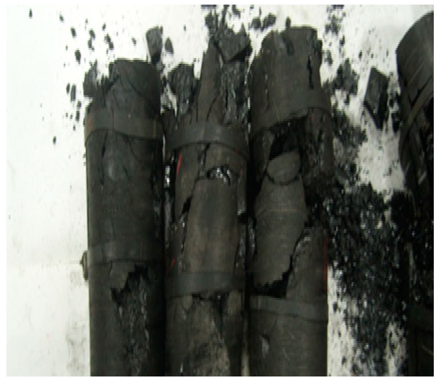
2.2. Mechanical Testing and Parameter Acquisition for Coal Samples

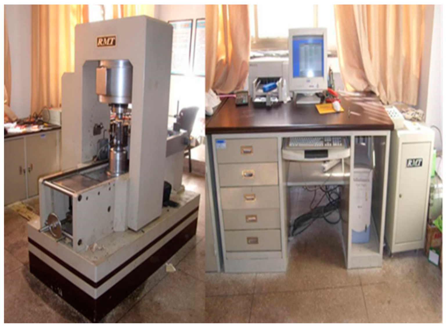
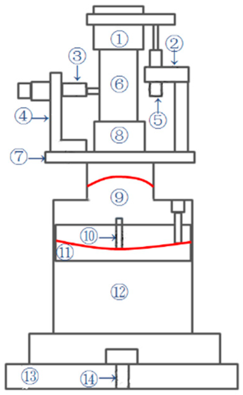
2.2.1. Introduction of RMT-150B Servo Tester

An RMT-150B rock mechanics multifunctional testing machine system was selected as the test loading equipment, as shown in Figure 3. The test machine was equipped with four types of sensors, namely stroke, stress, displacement and pressure, with fourteen sensors installed in total. The stroke sensor is used to monitor the stroke of the vertical hydraulic cylinder. The stress sensor is used to monitor the stress exerted by the vertical and horizontal hydraulic cylinders on the sample being tested. The displacement sensor is used to monitor the axial and lateral deformation of the specimen. The pressure sensor is used to monitor the pressure in the triaxial compression. The above sensors have the advantages of high precision and good stability, but human error or poor daily management and maintenance can lead to errors in the test results. Therefore, to avoid such errors, the testing machine is maintained by laboratory management personnel, and coal sample mechanical testing is performed by an experienced operator to obtain accurate and reliable test data.

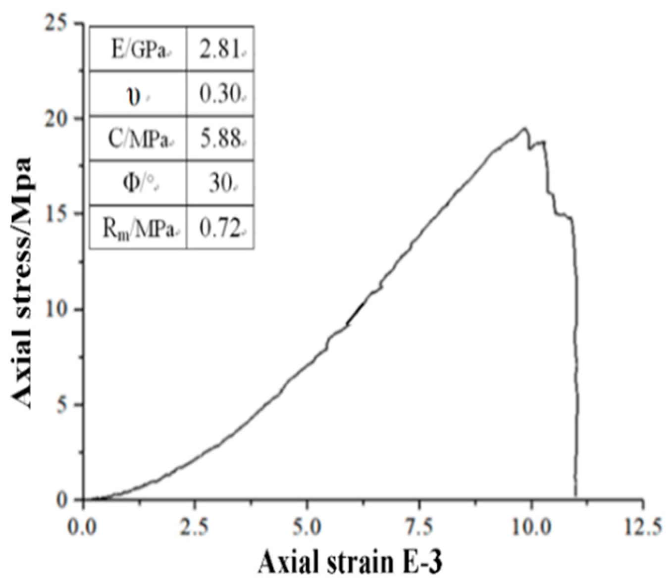
2.2.2. Mechanical Parameter Acquisition

Two test samples were damaged during processing and could not be used. Therefore, mechanical tests were carried out on the remaining twelve specimens: four specimens underwent uniaxial compression testing, three underwent the Brazilian splitting test and five underwent triaxial compression testing. The number of specimens tested is lower than the minimum suggested by ISRM to obtain reliable parameter estimates for the mechanical properties of rock. However, the mechanical parameters provide a reference data for the orthogonal test and the variation of the mechanical parameters has little influence on the results of orthogonal tests. Taking uniaxial compression testing as an example, a prepared specimen was placed on the pressure plate below the testing machine, and the axial and lateral displacement sensors were installed and adjusted, as shown in Figure 4.

Displacement control was adopted for the uniaxial compression test, with a loading rate of 0.02 mm/s, and loading was carried out under computer control until the specimen was damaged, as shown in Figure 5. The Brazilian splitting test was controlled by the stroke, with a loading rate of 0.005 m/min. A conventional triaxial compression test was adopted for triaxial compression testing, that is, σ₁ > σ₂ = σ₃, and the confining pressures were 2, 5, 10, 15 and 20 MPa. Displacement control was adopted for the triaxial testing. First, confining pressure was added in a static and horizontal manner, with a loading rate of confining pressure of 0.1 MPa/s. Then, axial pressure was added until the predetermined confining pressure value was reached, and the axial loading rate was 0.005 mm/s. The mechanical parameters and the stress–strain curve of the coal sample were automatically recorded by the computer, as shown in Figure 6.

The specific mechanical parameters are shown in

Table 1. Mechanical parameters of coal samples.

Test	E (GPa)	υ	UCS (MPa)	C (MPa)	Φ (°)	Ψ (°)	Rm (MPa)
Uniaxial compression test	3.20	0.35	20.6	/	/	/	/
	2.60	0.22	18.7	/	/	/	/
	2.19	0.33	15.7	/	/	/	/
	3.22	0.30	25.4	/	/	/	/
Brazilian splitting test	/	/	/	/	/	/	1.23
	/	/	/	/	/	/	0.12
	/	/	/	/	/	/	0.81
Triaxial test	/	/	/	10.88	40.5	/	/
	/	/	/			/	/
	/	/	/			/	/
	/	/	/			/	/
	/	/	/			/	/
Average	2.81	0.30	20.1	10.88	40.5	/
Adjusted parameter	2.81	0.30	20.1	5.88	30	8	0.72

, in which the C and Φ were calculated by the five tests of the Mohr–Coulomb strength criterion. To ensure an adequate simulation of the numerical test and facilitate the orthogonal calculation, the mean values of some parameters were reduced.

It is difficult to obtain an accurate Ψ through mechanical experiments, so Hoek and Brown [28] suggested that constant Ψ = Φ/4, Φ/8 and 0 should be used to describe the ideal post-peak behavior of rock masses, namely elasto-brittle, strain softening and ideal elastic–plastic deformation. Based on the mechanical test results of coal samples, this study determined that the Ψ is a constant value, Ψ = Φ/4. According to the classical plasticity theory, the Mohr–Coulomb strength criterion and the non-associated flow rule, it is assumed that the variation of material parameters is related to the softening parameters (plastic shear strain) [29,30,31]. Among them, the determination of FLAC3D numerical simulation softening parameters and material weakening method refer to the calculation formula in the literature [32] and the table command flow of FLAC3D numerical simulation is used to weaken the relevant parameters of strain softening (including C, Φ and Ψ).

2.3. Numerical Simulation Test

2.3.1. Establishment of Numerical Model

The FLAC3D numerical simulation software, as an extension of a finite difference program, can analyze the mechanical properties and plastic flow failure of rock and soil masses and can characterize well the nonlinear mechanical response characteristics of rock and soil [33,34].Therefore, in this study, the cylinder model (diameter 50 mm × height 100 mm) and the cuboid model (length 50 mm × width 50 mm × height 100 mm) were established by using FLAC3D finite difference software. Displacement loads at a constant rate were applied to the top and bottom of the model, and no boundary conditions were applied around it, as shown in Figure 7.

A coal sample is an anisotropic inhomogeneous body with voids and developed joints; therefore, the numerical model was simplified as an isotropic homogeneous body, while the time units of load applications used were different. The mechanical experiment units were mm/s or mm/min, and the FLAC3D units were mm/step. The loading rate of mechanical testing was directly applied to the numerical model, and the results of the numerical simulation were quite different from those of mechanical testing. This is because the specimen for gap, joint development of anisotropic heterogeneous body and the numerical simulation process model are simplified to ideal isotropic homogeneous body and there are no other deformations except for elastic deformation, such as crack closure and joint development. Therefore, the loading rate in mechanical testing could not be directly used in the numerical simulation. It is necessary to determine a reasonable model shape, a constitutive model, and a loading rate based on theoretical analysis and many numerical simulations. There was a heavy workload of numerical simulations, so in this paper we do not list them in detail but only analyze the typical results of each condition.

2.3.2. Constitutive Model Selection

The constitutive relation is used to represent the mechanical properties of materials in numerical simulation testing, and mechanical response characteristics vary considerably between different constitutive models. Therefore, it is important to select a constitutive model to study the mechanical characteristics of coal accurately. At present, strain-softening models and Mohr–Coulomb models are typically used in mechanical testing of coal/rock masses with FLAC3D [35,36,37,38].

The Mohr–Coulomb model is the conventional model used to represent compression-shear failure in soils and rocks. The failure envelope for this model corresponds to a Mohr–Coulomb criterion (shear yield function) with tension cutoff (tension yield function) [39]. Once the stress reaches the peak strength, the strength of rock will rapidly decrease as the deformation continues to increase; this is called “strain softening” [40]. Therefore, a numerical simulation test can not only reflect the elastic stage and yield failure of rock but also characterize the mechanical properties of rock after the peak. The strain-softening model allows representation of nonlinear material softening behavior based on prescribed variations of the Mohr–Coulomb model properties [39]. In FLAC3D, the strain softening model in the elastic stage is exactly the same as the Mohr–Coulomb model [41]. The difference, however, lies in the possibility that the C, Φ, Ψ and R_m may soften after the onset of plastic yield. In the Mohr–Coulomb model, those properties are assumed to remain constant [39]. The yield function, flow rule and stress correction of the strain softening model are consistent with those of the Mohr–Coulomb model [42].

The shear yield function of the strain softening model is:

$$f^s={\sigma }_1-{\sigma }_3{N}_{\phi }+2c\sqrt{N_{\phi }}$$

(1)

Here, σ₁ and σ₃ represent the maximum and minimum principal stresses, respectively; C is cohesion; φ is the internal friction angle; and N_φ is defined as follows.

$$N_{\phi }=\left(1+\sin \phi \right)/\left(1-\sin \phi \right)$$

(2)

In the case of shear failure, according to the orthogonal flow law, the stress of shear failure can be modified as follows:

$$\{\begin{array}{c}{\sigma }_1^N={\sigma }_1^I-{\lambda }^s\left({\alpha }_1-{\alpha }_2{N}_{\psi }\right)\hfill \\ {\sigma }_2^N={\sigma }_2^I-{\alpha }_2{\lambda }^s\left(1-N_{\psi }\right)\hfill \\ {\sigma }_3^N={\sigma }_3^I-{\lambda }^s\left({\alpha }_2-{\alpha }_1{N}_{\psi }\right)\hfill \end{array}$$

(3)

Here, σ₂ is the intermediate principal stress; σ₁ and σ₃ represent the maximum and minimum principal stresses, respectively; α₁ and α₂ are material constants defined in terms of the shear modulus and the bulk modulus, respectively; λ^t is the undetermined plasticity coefficient; superscripts N and I represent the new and old stress states of the element, respectively; Ψ is dilation angle; and N_ψ is defined as follows:

$$N_{\psi }=\left(1+\sin \psi \right)/\left(1-\sin \psi \right)$$

(4)

It can be seen from the stress–strain curve (Figure 6) obtained from the mechanical test of the coal sample that at the initial stage of loading, the axial strain of the coal sample increased rapidly due to the rapid closure of internal voids or micro cracks. With increasing applied load, the load was less than the yield strength, and the stress–strain curve essentially increased in a straight line, which showed that only reversible elastic deformation occurred in the specimen and that no plastic failure occurred. With a continuously increasing applied load, when the applied load approached the yield strength, the stress–strain curve began to show a concave shape, the specimen began to crack, and then it underwent irreversible plastic deformation. When the applied load reached the yield strength, the plastic failure range expanded rapidly, but the specimen retained a certain bearing capacity. However, the bearing capacity gradually decreased with increasing strain, showing a significant strain softening phenomenon. When the strain reached a certain value, the stress–strain curve rapidly decreased, which was mainly caused by the brittleness of the coal sample. Based on the above analysis, the strain softening model can better simulate the mechanical properties of coal samples.

In the process of numerical simulation, to solve the problem of weakening parameters such as C and Φ in the strain softening stage, the formula in [32] can be used:

$${{\rm N}}_{\psi }{\epsilon }_1^p+2{\epsilon }_3^p=0$$

(5)

$$\eta ={\epsilon }_1^p-{\epsilon }_3^p$$

(6)

$$K\left(\eta \right)=\{\begin{array}{ll}{K}_p-\frac{K_p-K_1}{{\eta }_1}\eta & 0\le \eta \le {\eta }_1\\ K_1-\frac{K_1-K_2}{{\eta }_2-{\eta }_1}\left(\eta -{\eta }_1\right)& {\eta }_1\le \eta \le {\eta }_2\\ \cdots \cdots \\ K_{n-1}-\frac{K_{n-1}-K_r}{\eta *-{\eta }_{n-1}}\left(\eta -{\eta }_{n-1}\right)& {\eta }_{n-1}\le \eta \le \eta *\end{array}$$

(7)

where ${\epsilon }_1^p$ is the axial plastic main strain; ${\epsilon }_3^p$ is the lateral plastic main strain; η is the softening coefficient; K represents C and Φ; p represents peak mechanical parameters; r represents residual mechanical parameters; η₁, η₂, …, η_n−1 are the softening parameter at the end of stages 1, 2, …, n − 1; and η* is the softening parameter when the discharge reaches the residual state.

Combined with the results of the mechanical test shown in Table 1, the softening coefficients (η) of mechanical parameters at different stages can be obtained by Formulae (4)–(7), as shown in

Table 2. Variation of coal sample strength parameters at different stages.

	C/MPa	Φ/°	η
Cumulative plastic strain 0	5.88	30	0
Cumulative plastic strain 0.008	5.76	28.06	0.0133
Cumulative plastic strain 0.015	1.42	26.24	0.0250

.

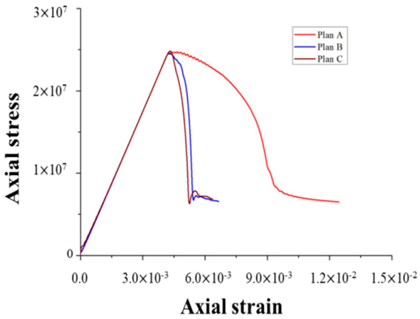
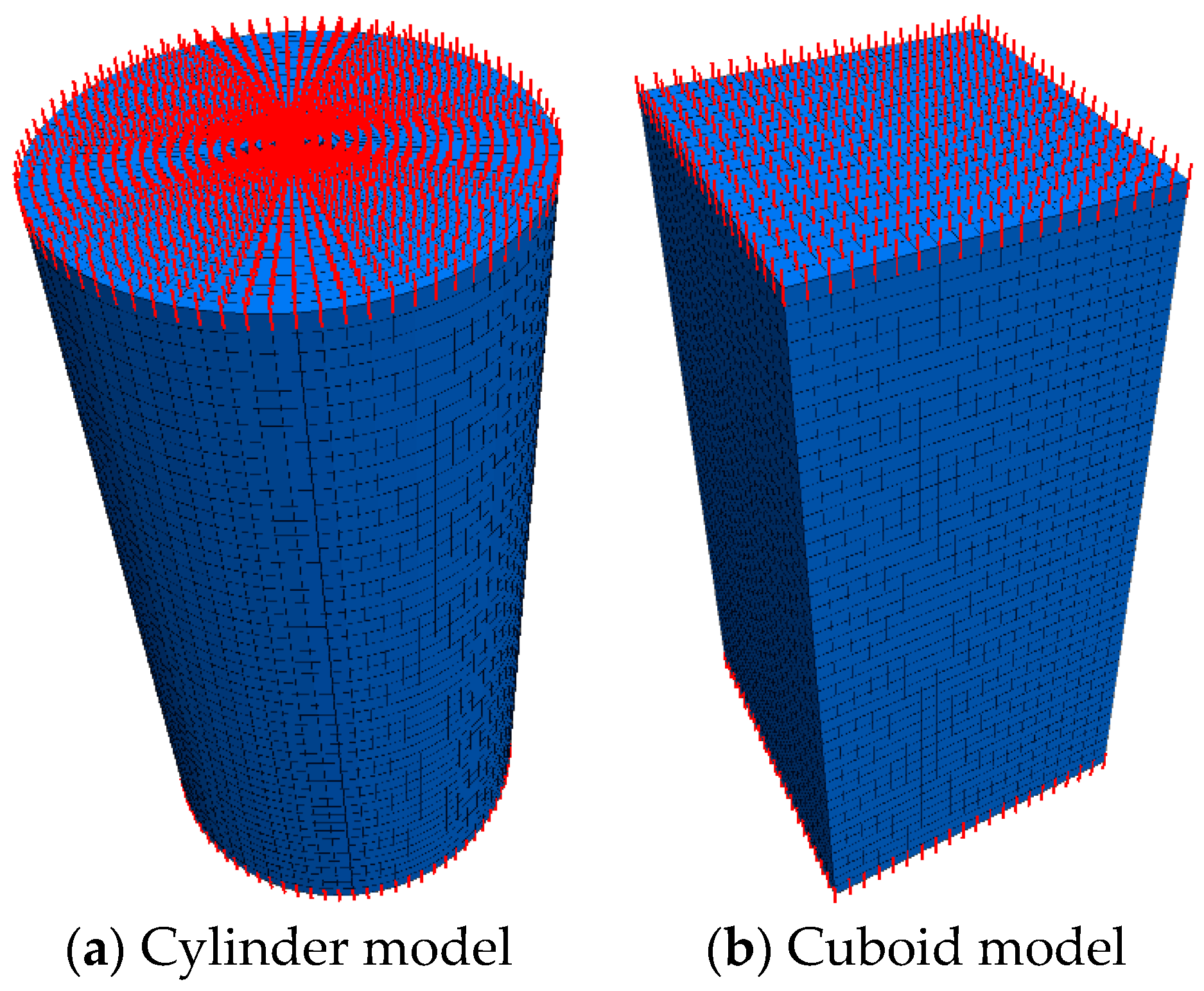
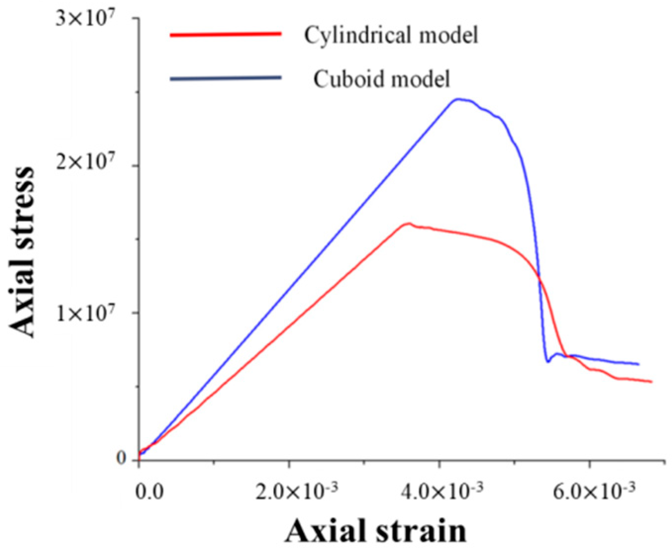
2.3.3. Model Shape Selection

In general, uniaxial compression test specimen shapes include cylinders (50 mm × 100 mm) and cuboids (50 mm × 50 mm × 100 mm). In this experiment, two models of cylinder and cuboid were established. The model adopted the weakened mechanical parameters in Table 1. The loading rates at the top and bottom were both 1.9 × 10⁻⁵ mm/step. The stress–strain curve of the numerical model is shown in Figure 8.

From the numerical simulation results, it can be seen that the cylinder model and the cuboid model underwent the same changes in the elastic stage, but their mechanical properties were quite different after the peak. The weakening process of the cylinder model was slow after the peak. However, the strength of the cuboid model after the peak rapidly decreased after the initial slow fluctuations, which accurately simulated the brittle failure of the coal body, and was consistent with the mechanical testing results of the coal sample, as shown in Figure 6. In addition, the yield strength of the cylinder model was 16.5 MPa and that of cuboid model was 24.4 MPa. The numerical model is homogeneous while coal samples are heterogeneous, with joints and voids; therefore, it is normal for the yield strength of the numerical simulation to be slightly higher than that of the mechanical experiment. Therefore, the cuboid model was selected for the orthogonal numerical simulation test.

2.3.4. Mesh Number of Model Element Body Is Determined

In FLAC3D software, the strain softening model is used to determine the degree of softening of the specimen parameters through the accumulated plastic strain after the peak, reflecting the mechanical properties of the specimen after the peak. The size of the model grid has an important influence on the development of plastic failure in test samples. If the grid size is too large, it can indirectly enhance the strength of the test sample, making it harder to damage it. If the grid size is too small, it is too sensitive to loads and the specimen is weak and easy to damage. In this study, three grid sizes were designed: Scheme A, grid size 5 mm long × 5 mm wide × 2 mm high, with 5000 grids divided for test samples; Scheme B, grid size 2.5 mm long × 2.5 mm wide × 2 mm high, with 20,000 grids divided for test samples; and Scheme C, grid size 1 mm long × 1 mm wide × 2 mm high, with 125,000 grids divided for test samples. The stress–strain curves of different mesh sizes obtained by numerical simulation are shown in Figure 9.

According to the comparison of Figure 6 and Figure 9, the post-peak failure processes of the different schemes were quite different. In Scheme A, the post-peak softening modulus of the sample was small and could not accurately simulate the brittleness of the post-peak failure of coal samples. The post-peak softening modulus of Schemes B and C was relatively large, which could simulate the brittleness characteristics of coal samples. However, when comparing these two schemes, the stress–strain curve of Scheme B rapidly decreased following a short fluctuation, while Scheme C decreased directly and rapidly after the peak. Scheme B was more consistent with the mechanical properties of coal samples (Figure 6). Therefore, Scheme B was selected for this simulation: the grid size was 2.5 mm long × 2.5 mm wide × 2 mm high, and 20,000 grids were divided for test samples.

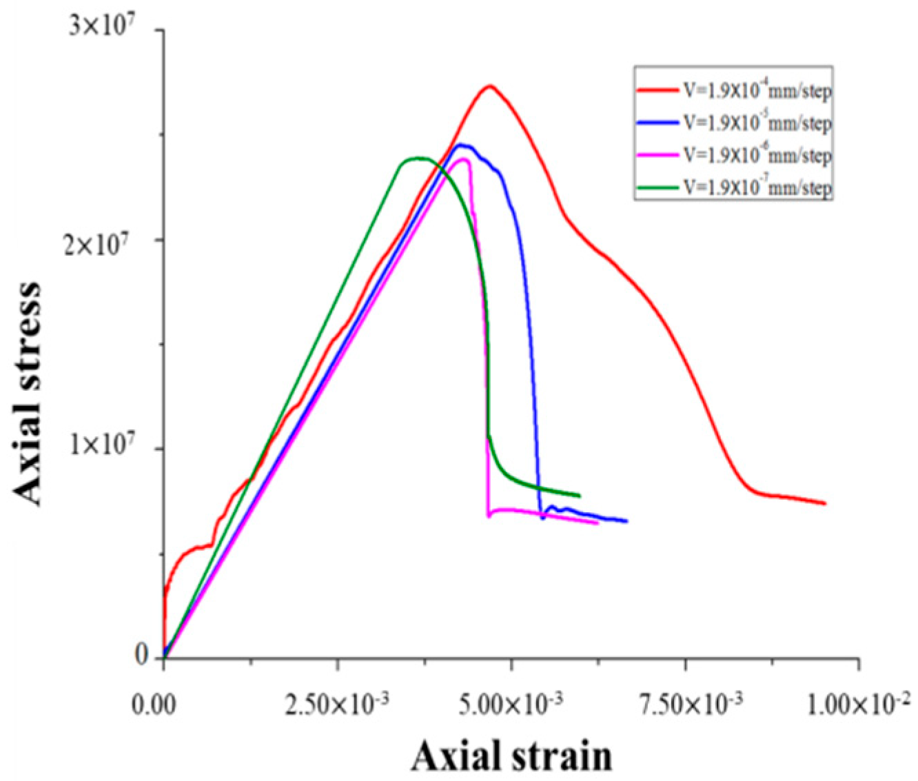
2.3.5. Loading Rate Determination

The results show that different loading rates exerted a great influence on the strength and failure modes of rock mass. It has been shown that the peak strength of rock increases with increasing loading rate [43]. Through mechanical testing, it has been shown that the peak strength of a coal sample first increases and then decreases with the increase in loading rate [44]. Through Particle Flow Code (PFC) numerical simulation testing, it was found that the UCS of coal samples increases with increased loading rate, and that the failure mode changes from X-shaped, V-shaped or Y-shaped to a single macroscopic fracture surface [45]. In addition, the unit used for the acceleration rate in mechanical testing and numerical simulation loading is different. The unit of mechanical testing is mm/s or mm/min, and the unit of FLAC3D is mm/step. Therefore, the loading rate of mechanical test cannot be directly applied to numerical simulation. To make the simulation test results more accurate and constant with the mechanical properties of coal samples, it is necessary to discuss the reasonable value of the acceleration rate. The loading rates were 1.9 × 10⁻⁴, 1.9 × 10⁻⁵, 1.9 × 10⁻⁶ and 1.9 × 10⁻⁷ mm/step, and the remaining numerical simulation conditions remained consistent. The stress–strain curves of the numerical models with different loading rate conditions were recorded, as shown in Figure 10.

It can be known from the stress–strain curves of different loading rates, from the yield strength, when the loading rate V = 1.9 × 10⁻⁴ mm/step, the yield strength is 27.3 MPa. Compared with the mechanical test results in Table 1, the deviation rate is 35.82%. When the loading rate V = 1.9 × 10⁻⁵ mm/step, the yield strength is 24.4 MPa and the deviation rate is 21.39%. When the loading rate V = 1.9 × 10⁻⁶ mm/step, the yield strength is 23.8 MPa and the deviation rate is 18.41%. When the loading rate V = 1.9 × 10⁻⁷ mm/step, the yield strength is 24.0 MPa and the deviation rate is 19.4%. Therefore, when the loading rate was low, the yield strength tended to be stable. When the loading rate was more than 1.9 × 10⁻⁵ mm/step, the yield strength of the numerical model rapidly increased with the loading rate. Due to the low loading rate, the load of the model was similar to the static load, and the internal damage and plastic damage of the model had sufficient time to develop, thus the yield strength was low and the difference was small. With an increase in loading rate, the plastic failure time decreased, the degree of damage in the model decreased and the strength continuously increased [44]. From the mechanical performance curve, when the loading rate V = 1.9 × 10⁻⁴ mm/step, after the model reaches the yield strength, the axial stress gradually decreases with the increase of axial strain. When the loading speeds were V = 1.9 × 10⁻⁵ and 1.9 × 10⁻⁷ mm/step, when the model reached the yield strength, as the strain increased, the stress decreased, slowly at first and then rapidly. When the loading speed was V = 1.9 × 10⁻⁶ mm/step, the axial stress rapidly decreased and the brittleness increased after the model reached the yield strength. Compared with the stress–strain curve of the coal sample in Figure 6, the stress–strain curve and the mechanical properties of the loading rate V = 1.9 × 10⁻⁵ and 1.9 × 10⁻⁷ mm/step were more consistent with the mechanical test results of the coal sample. However, when the loading rate was V = 1.9 × 10⁻⁷ mm/step, the simulation time of a single model was significantly longer than for a rate of 1.9 × 10⁻⁵ mm/step. Based on the comparative analysis of the four loading rates, the selected loading rate of orthogonal numerical simulation test is 1.9 × 10⁻⁵ mm/step.

2.4. Orthogonal Experimental Method and Experimental Scheme

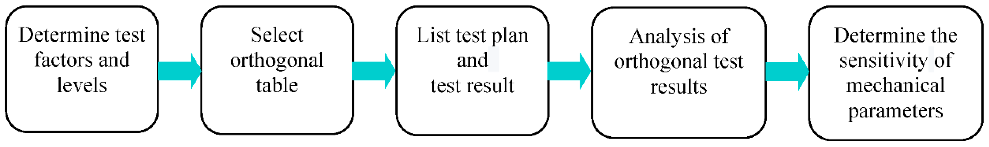
2.4.1. Orthogonal Experimental Method

The orthogonal experimental method involves an overall design, comprehensive comparison and statistical analysis of a test carried out in an orthogonal table. It also includes representative test points selected from a large set of test data; these test points go through testing, comprehensive comparison and summary analysis via the orthogonal table. The specific design process is shown in Figure 11. The whole process of the experiment ensures that different levels of each parameter are considered the same number of times in the scheme and that different combinations of any two parameters occur the same number of times. Therefore, the uniformity and rationality of multiple parameters at different levels can be guaranteed, as can the reliability and representativeness of test results. Additionally, the number of tests conducted can be reduced significantly without affecting the feasibility of the test results. Thus, ideal test results can be achieved based on fewer representative test points, the sensitivity of each parameter to the test results can be determined and optimal test results can be obtained with the minimum number of tests [46].

2.4.2. Orthogonal Experimental Research Level and Scheme Design

Based on the mechanical properties and constitutive relations of the coal samples, the six mechanical parameters (E, υ, C, Φ, R_m and Ψ) measured in Table 1 were taken as the initial participating factors of the orthogonal experiment. Based on the results of previous studies considering the horizontal spacing of different parameters in orthogonal experiments [47,48], it was determined that each participating parameter in this experiment has 5 typical levels, with horizontal spacings of 1 GPa, 0.02, 2 MPa, 2°, 0.5 MPa and 1° for E, υ, C, Φ, R_m and Ψ, respectively. The specific parameters adopted are presented in

Table 3. Research level of orthogonal numerical simulation experimental parameters.

	A	B	C	D	E	F
	E (GPa)	υ	C (MPa)	Φ (°)	Rm (MPa)	Ψ (°)
1	2.81	0.30	5.88	30	0.72	8
2	3.81	0.32	7.88	32	1.22	9
3	4.81	0.34	9.88	34	1.72	10
4	5.81	0.36	11.88	36	2.22	11
5	6.81	0.38	13.88	38	2.72	12

.

According to the orthogonal experiment design, a permutation combination scheme with six parameters at five levels and twenty-five orthogonal numerical simulation schemes (L₂₅ (5⁶)) was selected. The primary purpose of this experiment was to study the influence of the selected mechanical parameters on UCS and PS. The main controlling parameters were determined; UCS was monitored and PS was recorded for different parameters and multiple levels in the numerical simulation test, as shown in

Table 4. Orthogonal numerical simulation experimental schemes.

Experimental Scheme	Mechanical Parameters						Simulation Results
	E (GPa)	υ	C (MPa)	Φ (°)	Rm (MPa)	Ψ (°)	UCS (MPa)	PS (10−3)
1	2.81	0.30	5.88	30	0.72	8	20.1	3.61
2	2.81	0.32	7.88	32	1.22	9	27.9	4.88
3	2.81	0.34	9.88	34	1.72	10	36.1	5.99
4	2.81	0.36	11.88	36	2.22	11	44.9	7.65
5	2.81	0.38	13.88	38	2.72	12	54.4	9.06
6	3.81	0.30	7.88	34	2.22	12	29.2	3.78
7	3.81	0.32	9.88	36	2.72	8	37.7	4.95
8	3.81	0.34	11.88	38	0.72	9	47.0	6.06
9	3.81	0.36	13.88	30	1.22	10	46.9	6.01
10	3.81	0.38	5.88	32	1.72	11	20.9	2.78
11	4.81	0.30	9.88	38	1.22	11	39.5	4.14
12	4.81	0.32	11.88	30	1.72	12	40.6	4.23
13	4.81	0.34	13.88	32	2.22	8	49.0	5.03
14	4.81	0.36	5.88	34	2.72	9	21.9	2.34
15	4.81	0.38	7.88	36	0.72	10	30.2	3.15
16	5.81	0.30	11.88	32	2.72	10	42.3	3.75
17	5.81	0.32	13.88	34	0.72	11	51.2	4.36
18	5.81	0.34	5.88	36	1.22	12	22.9	2.09
19	5.81	0.36	7.88	38	1.72	8	31.5	2.75
20	5.81	0.38	9.88	30	2.22	9	40.5	3.47
21	6.81	0.30	13.88	36	1.72	9	53.3	3.95
22	6.81	0.32	5.88	38	2.22	10	23.9	1.85
23	6.81	0.34	7.88	30	2.72	11	27.2	2.05
24	6.81	0.36	9.88	32	0.72	12	35.2	2.67
25	6.81	0.38	11.88	34	1.22	8	43.8	3.20

.

3. Effect of Mechanical Parameters on UCS and PS

3.1. Influence Analysis of Mechanical Parameters on UCS

The range index was introduced to analyze the influence of mechanical parameters on UCS, based on orthogonality and the comprehensive comparability of the orthogonal experiment, both for additional analysis and to allow comprehensive comparability of the results with the orthogonal experiment. Range is used to express the variation in statistical data and to represent the difference between maximum and minimum values in the calculated mean UCS for a fixed value of one of the six parameters used in the orthogonal analysis. The size of the range reflects the degree of influence each parameter has under different levels of change; thus, it determines the degree of influence each parameter has on UCS and reveals how UCS varies with different parameters. The mean value and range of UCS for different values of various parameters were calculated from Table 4, as shown in

Table 5. Average and range for different values of each parameter.

UCS (MPa)	A	B	C	D	E	F
	E (GPa)	υ	C (MPa)	Φ (°)	Rm (MPa)	Ψ (°)
Average 1	36.68	36.88	21.94	35.06	36.74	36.42
Average 2	36.34	36.26	29.20	35.06	36.20	38.12
Average 3	36.24	36.44	37.80	36.44	36.48	35.88
Average 4	37.68	36.08	43.72	37.80	37.50	36.74
Average 5	36.68	37.96	50.96	39.26	36.70	36.46
Range	1.44	1.88	29.02	4.20	1.30	2.24

.

As illustrated in Table 4, the ranges of E, υ, R_m, Ψ and Φ are 1.44, 1.88, 1.30, 2.24 and 4.20, respectively. In contrast, the range of C is 29.02. Thus, these results show that C has the greatest influence on UCS, followed by Φ, while E, υ, R_m and Ψ have relatively little influence on UCS.

To more intuitively demonstrate the influence of each parameter on UCS, curve diagrams were produced to illustrate changes in horizontal compressive strength with changes in the average value (Table 5) of the corresponding compressive strength for each parameter in Table 4. To facilitate comparative analysis of the degree of influence of each parameter on UCS, the ordinate range of the six parameters included in the curve diagrams was determined to be 20~52 MPa, and close-up plots were produced for the parameters with relatively small amplitude changes, as shown in Figure 12.

The following can be inferred based on the information presented in Table 5 and Figure 12.

(1)

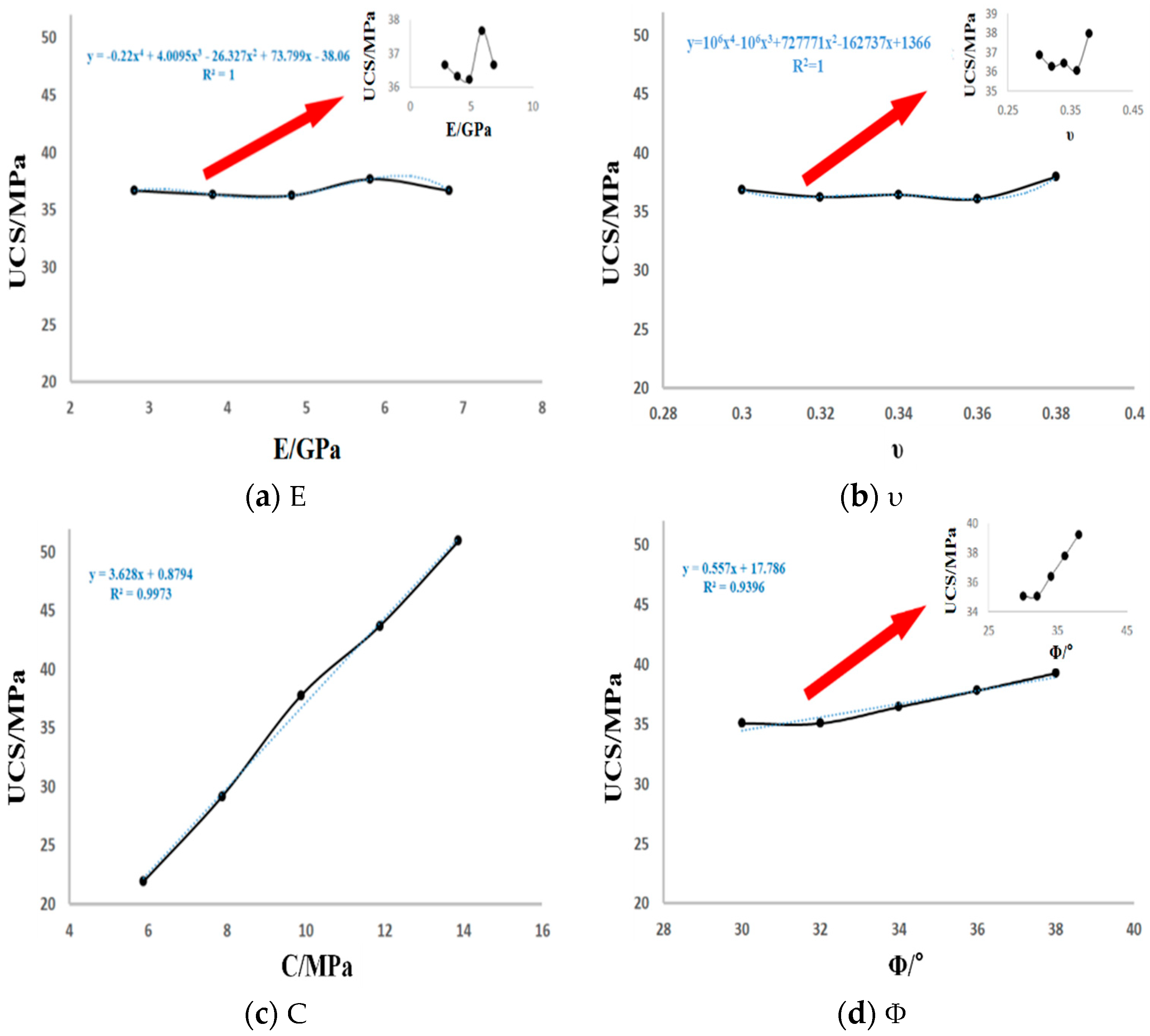
When E increases from 2.81 to 6.81 GPa, the change in UCS is minimal and the stress value fluctuates within the range 36~37 MPa. Therefore, the influence of the elastic modulus on UCS is small. According to the smaller range between axis limits, a nonlinear relationship exists between E and UCS. With increasing E, compressive strength first decreases before increasing and then decreasing again; however, the fluctuation range is small, indicating that there is a relatively stable critical range of UCS for different values of E, as shown in Figure 12a.

(2)

With increasing υ, UCS exhibits a fluctuating curve. In the early stage, when υ increases from 0.30 to 0.36, UCS exhibits a decrease followed by an increase and a subsequent decrease, although the maximum change range is only 0.8 MPa. Conversely, in the later stage, when υ increases from 0.36 to 0.38, the compressive strength increases from 36.08 to 37.96 MPa; this increase of 1.88 MPa is relatively pronounced. Thus, when υ is small, changes in UCS are comparatively small and UCS is not sensitive to changes in Poisson’s ratio; conversely, when υ is comparatively large, the sensitivity of UCS to changes in υ increases, as shown in Figure 12b.

(3)

C has a considerable influence on UCS for the coal samples, with UCS ranging from 21.94 to 50.96 MPa for different C levels. Based on curve for this specific analysis, the fitting equation between C and UCS is y = 3.628x + 0.8794, with R² = 0.9973. There is a clear linear relationship between C and UCS, with a range of 29.02. Thus, UCS is sensitive to changes in C, increasing linearly. The results also illustrate that UCS does not converge to a critical range with variation in C, as shown in Figure 12c.

(4)

The influence of Φ on UCS can be divided into two stages: when Φ is less than 32°, UCS remains essentially unchanged with increasing Φ; conversely, when Φ is greater than 32°, UCS increases rapidly with increasing Φ and there is a significant linear growth relationship between the two variables. Thus, Φ has a significant impact on UCS and the degree of its influence is relatively large. Based on a comprehensive consideration of the whole curve, a nonlinear relationship exists between UCS and Φ: when Φ exceeds 32°, UCS increases linearly with increasing Φ and UCS does not have a stable critical range, as shown in Figure 12d.

(5)

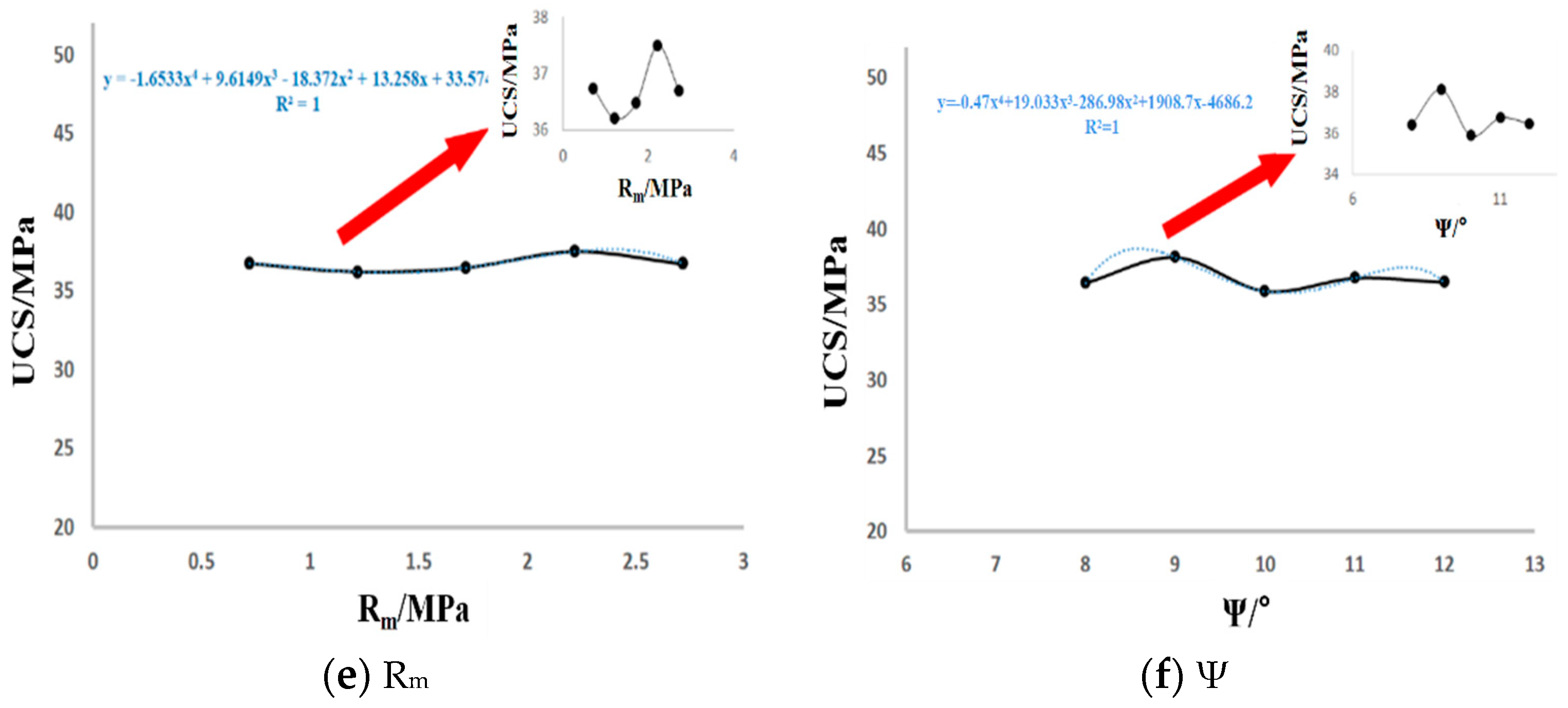
Based on the relationship between R_m and UCS, changes in the range of UCS with increasing Rm are very small, with minimum and maximum values of 36.2 and 37.5 MPa, respectively (a range of only 1.3 MPa). Therefore, Rm has little influence on UCS. There is a significant nonlinear relationship between the two variables according to the microscopic analysis diagram, as shown in Figure 12e.

(6)

The relationship between Ψ and UCS indicates that, when Ψ is less than 10°, UCS first increases from 36.42 to 38.12 MPa and then decreases to 35.88 MPa with increasing Ψ (a range of 2.24 MPa). Conversely, when Ψ is greater than 10°, UCS increases from 35.88 to 36.74 MPa and then decreases to 36.46 MPa (a range of 0.86 MPa). This indicates that a nonlinear relationship exists between Ψ and UCS, with the influence of Ψ on UCS being more pronounced for small values of Ψ, as shown in Figure 12f.

3.2. Influence Analysis of Mechanical Parameters on PS

Along with strength properties, the deformation properties of coal can be considered critical mechanical properties. The deformation and failure of coal masses often affect both the stability of rock surrounding roadways and the dynamic strength of the rock mass during the process of coal mining. Therefore, it is of great importance to be able to control rock surrounding roadways and prevent dynamic disasters by understanding fully deformation and failure laws and the mechanical response characteristics of coal.

Based on stress–strain curves, the deformation of coal goes through three stages before reaching UCS: the compaction stage, the elastic stage and the plastic stage. There is a positive correlation between the stress and strain of coal masses during this process: the greater the deformation of the coal mass, the greater the required stress. When the coal mass reaches UCS, the bearing capacity of the coal mass reaches its maximum; after exceeding UCS, the stress decreases with increasing strain, exhibiting an obvious strain softening phenomenon, as shown in Figure 13. Therefore, the strain corresponding to the coal mass peak is the PS, and its magnitude has a vital influence on the mechanical response of the coal mass when it is damaged. The brittle characteristics of coal failure are dominant for low PS, which is prone to inducing dynamic disaster; conversely, the plastic characteristics are dominant for higher PS, which is prone to inducing large-scale deformation of the rock surrounding roadways [49,50]. This demonstrates that PS is one of the major indices able to characterize the mechanical response of coal masses.

Based on the orthogonal experiment results presented in Table 4, the mean and range of PS at different levels of each parameter considered were obtained, as shown in

Table 6. Statistics describing the influence of mechanical parameters on PS.

PS (10−3)	A	B	C	D	E	F
	E (GPa)	υ	C (MPa)	Φ (°)	Rm (MPa)	Ψ (°)
Average 1	6.24	3.85	2.53	3.87	3.97	3.91
Average 2	4.77	4.05	3.32	3.82	4.06	4.14
Average 3	3.78	4.24	4.24	3.93	3.94	4.15
Average 4	3.28	4.28	4.98	4.36	4.36	4.20
Average 5	2.74	4.33	5.68	4.78	4.43	4.37
Range	3.50	0.48	3.15	0.96	0.49	0.46

.

According to Table 6, the ranges in E and C are 3.50 and 3.15, respectively. It can be seen that E has the most pronounced influence on PS, followed by C; the ranges of υ, Φ, R_m and Ψ are relatively small, and their influences on PS are also small. To more intuitively characterize the influence of various mechanical parameters on PS, curves were plotted to illustrate the relationships between these parameters and PS and the ordinates of all curves were unified with the same max and min values on the y-axis. Smaller ranges between axis limits were produced for the parameters with lower sensitivity, as shown in Figure 14.

The following inferences can be made based on Table 6 and Figure 14.

(1)

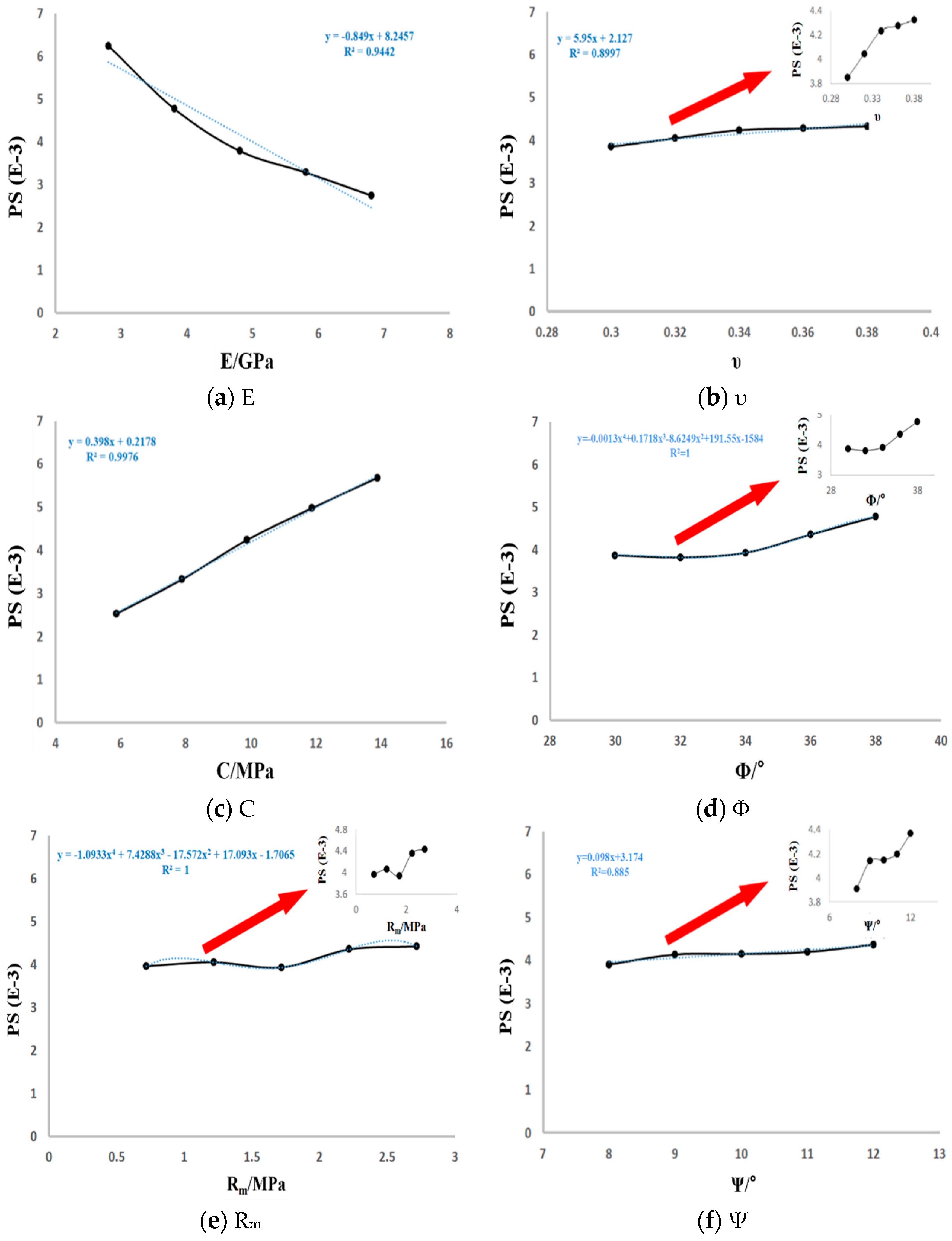
Based on the curve in Figure 14a, the relationship between E and PS is approximately linear. When the other parameters remain constant, PS decreases with increasing E, which is closely related to the deformation resistance of the object as characterized by E. For large values of E, the deformation resistance is greater and the deformation is less pronounced; conversely, for smaller values of E, the deformation resistance is lesser and the deformation is more pronounced.

(2)

PS increases slowly with increasing υ from 0.30 to 0.38; thus, the overall change in PS is small and the sensitivity of PS to υ can be considered relatively small. A smaller range between axis limits indicates that PS growth with increasing Poisson’s ratio occurs in two stages: in the first stage, υ increases from 0.3 to 0.34 and the PS growth rate is 10.13%; in the second stage, υ increases from 0.34 to 0.38 and the PS growth rate is only 2.12%. The growth rate of PS in the second stage is significantly lower than that in the first stage, although a relatively significant linear relationship exists between υ and PS in each stage, as shown in Figure 14b.

(3)

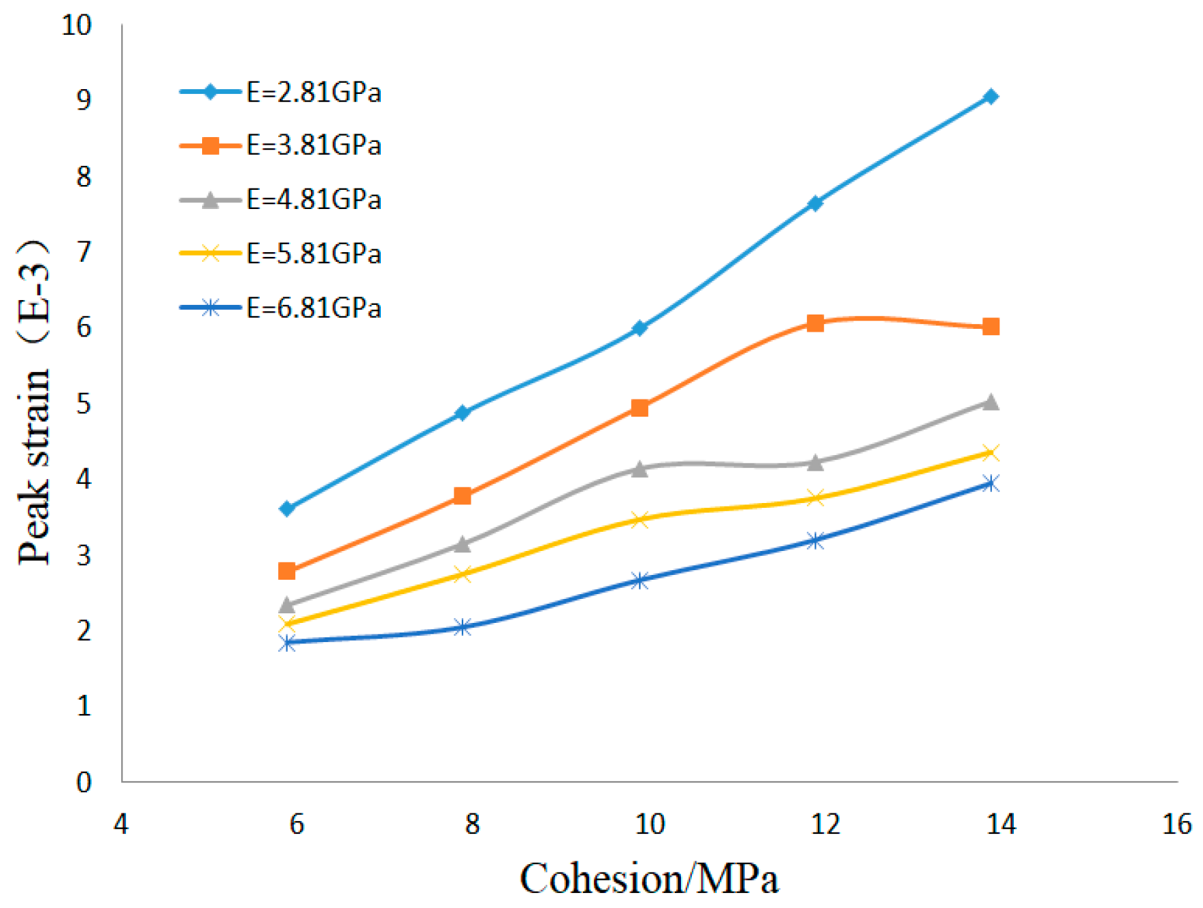
According to Figure 14c, PS increases linearly from 2.53 to 5.68 (range of 3.15) with increasing C. Other than E, C can be considered to have the largest influence on PS.

(4)

The influence of Φ on PS can also be considered to exhibit two stages. When Φ is less than 34°, the fluctuation range of PS is very small with increasing Φ and Φ thus has no effect on PS. Conversely, when Φ is greater than 34°, PS increases linearly with increasing Φ and the degree of influence of Φ on PS is greater, as shown in Figure 14d.

(5)

The influence of R_m on PS is variable, with no obvious regularity; the range is only 0.49 and R_m has little influence on PS. However, PS tends broadly to increase with increasing R_m, as shown in Figure 14e.

(6)

Based on the curve plotting PS against Ψ, PS increases from 3.91 to 4.37 as Ψ increases from 8° to 12°. This fluctuation range is small, indicating that the influence of Ψ on PS is small. Although the main plot indicates a lack of any clear linear relationship between Ψ and PS, the microscopic analysis diagram indicates that PS increases linearly with increasing Ψ before leveling off, and then exhibiting a further linear increase with Ψ at higher values of Ψ, as shown in Figure 14f.

The relationship between C and PS has been plotted for different values of E, as shown in Figure 15. The influence of C on PS is closely related to E. When E is 2.81 GPa, PS increases from 3.61 to 9.06 (range of 5.45) as C increases from 5.88 to 13.88 MPa; conversely, when E is 6.81 GPa, PS increases from 1.85 to 3.95 (range of 2.1) for the same range of C. Thus, the influence of C on PS decreases with increasing E. Overall, C and PS exhibit a linear relationship regardless of the value of E.

3.3. Influence Analysis of Mechanical Parameters on Critical Failure Strength of Coal Samples

For the whole stress–strain curve, UCS represents the maximum load-bearing capacity of the coal mass, and PS can be used to describe the deformation characteristics of the coal mass under uniaxial compression failure. Therefore, both PS and UCS can be used to characterize the critical failure strength of a coal mass.

Based on analysis of the influence of mechanical parameters on UCS and PS for coal masses, the degree of influence of the mechanical parameters on UCS decreases in the following order: C > Φ >Ψ> υ > E > R_m. Conversely, the degree of influence of these parameters on PS decreases in the following order: E > C > Φ > R_m > υ >Ψ. Thus, these mechanical parameters have different influences on UCS and PS. To more fully reveal the influence of these parameters on UCS and PS, a normalization method was used to map all range data presented in Table 5 and Table 6 onto the range 0~1, as shown in

Table 7. Normalized range of each parameter corresponding to peak stress and peak strain.

	E	υ	C	Φ	Rm	Ψ
Range (UCS)	1.44	1.88	29.02	4.20	1.30	2.24
Range (PS)	3.50	0.48	3.15	0.96	0.49	0.46
Range normalization (UCS)	0.036	0.047	0.724	0.105	0.032	0.056
Range normalization (PS)	0.387	0.053	0.349	0.106	0.054	0.051

. The normalization method is to scale the data that need to be processed to a small specific interval. To facilitate data processing, the data were mapped to a range of 0~1 for processing. The normalization results are plotted as a histogram for processing and comparison, as shown in Figure 16.

According to this comparative analysis, only C has an important influence on both UCS and PS, and E has a significant influence only on PS. The parameter Φ has the same influence on UCS as on PS, and all other mechanical parameters considered have a relatively small influence on both UCS and PS. The results illustrate that C has the greatest influence on the critical failure strength of coal masses under compression, and that increased cohesion can improve the critical failure strength of coal significantly. Thus, it can be inferred that the stability of rock surrounding roadways can be enhanced effectively by grouting and anchoring to improve C in the rock mass.

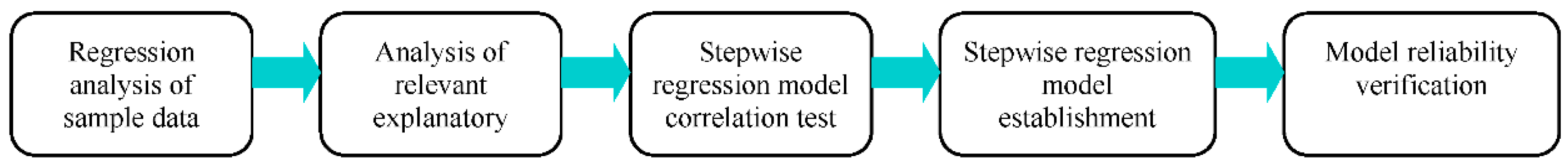
4. Stepwise Regression Prediction of UCS

According to the analysis described above, different mechanical parameters have different degrees of influence on UCS: C has the greatest influence on UCS, followed by Φ, with the influence of other mechanical parameters being relatively small. Based on this, a regression equation was derived by establishing a predictive model of UCS using stepwise regression analysis, and the main controlling parameters were used for rapid prediction of UCS, in order to obtain relatively accurate prediction of values with fewer variables. The technical workflow for this is shown in Figure 17.

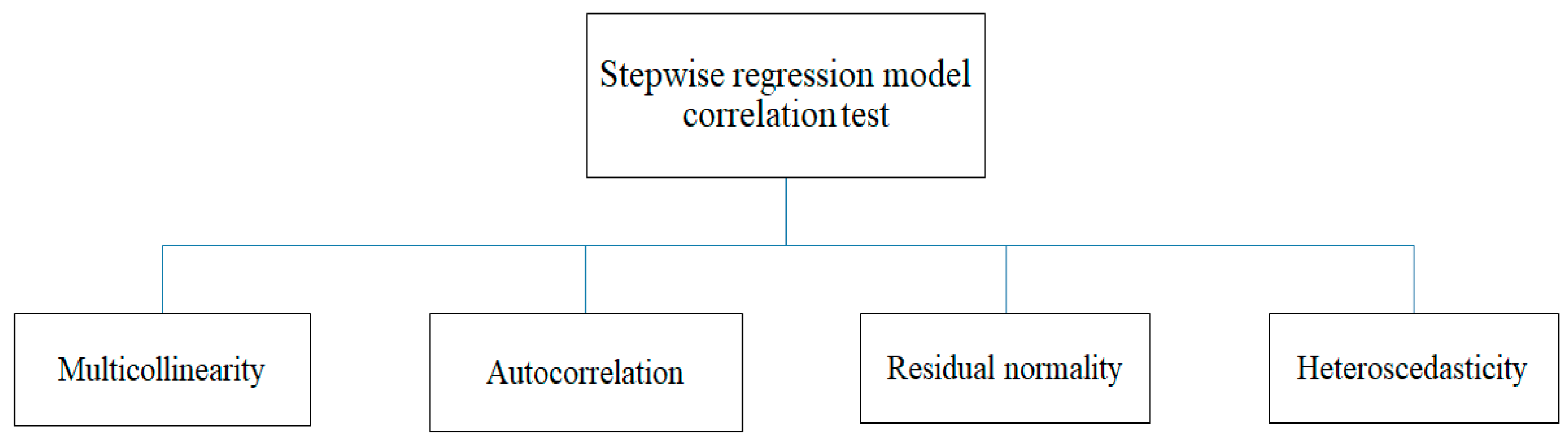
4.1. Stepwise Regression Equation Analysis of Relevant Explanatory Variables and Regression Model Establishment

The stepwise regression method is introducing all the independent variables into the regression model and determining the significance level of each independent variable. Eliminating the non-significant independent variables and reducing the number of independent variables are advantageous to the fast predicting of the changing trend of dependent variables. At the same time, using the identified significant independent variables to establish the regression equation, the optimal interpretive parameter set can be obtained.

Firstly, SPSS software was used to introduce all the participating factors into the regression model one by one. F test is generally used to compare the prediction model to the dataset for each factor and determine whether there is a significant difference in the correlation between the dependent variable and the independent variable. At the same time, the Student’s t-test was performed for the factors with obvious significance. When the significance level of other variables decreases due to the introduction of new variables, the model will automatically remove the variables with decreased significance, until no significant variables participate in the regression equation and no insignificant variables are removed by the equation, thus only the independent variables with significant effect are finally retained. In this paper, SPSS software was used to determine the independent variables of significance as C and Φ. Meanwhile, explanatory parameters of correlation regression test were recorded, including Variance Inflation Factor (VIF) value for multiple linear test, Durbin–Watson (D–W) value for autocorrelation in the residuals from the statistical regression analysis test, residual normality test and heteroscedasticity test. The specific parameters are shown in

Table 8. Related interpretation parameter sets of stepwise regression analysis.

	Non-Standardized Coefficient		Standardization Coefficient	t	p	VIF	R2	Adjusted R2	F
	B	Standard Error	Beta
Constant	−18.059	3.704	-	−4.876	0.000 **	-	0.983	0.981	619.574 (0.000 **)
C	3.628	0.104	0.980	34.79	0.000 **	1.000
Φ	0.557	0.104	0.150	5.342	0.000 **	1.000

Supplement: dependent variable—UCS. D–W value: 1.829. ** p < 0.01. Thank you for your advice.

.

In Table 8, the value of the non-standardized coefficient B is the value of the regression coefficient. B > 0 indicates that the influence of the independent variable on the dependent variable is positive and significant when p < 0.05, and the standard error indicates the degree of fluctuation of the regression coefficient. The standardized coefficient is the value of the regression coefficient for the related independent variable when the constant is 0; the t value is the intermediate variable for calculating the p value, and the p value is used to test the significance level of the coefficient. The smaller is the p value, the greater is the significance. R² indicates the explanatory power of the independent variable with respect to the dependent variable; that is, it demonstrates the goodness of fit of the regression equation. The closer R² is to 1, the more accurate is the model and the better is the fit of the regression equation. For this regression analysis, R² = 0.983, which demonstrates that C and Φ can accurately represent changes in UCS. The adjusted R² excludes the influence of increases in the independent variable on the goodness of fit of the model. The model was checked using the F value test (F = 619.574, p < 0.05), which indicated that the regression model is effective: in the table, the * symbol against the F value indicates that at least two independent variables have an impact on the dependent variable. The basic parameters of the model thus meet the relevant standards, based on the analysis of related parameters considered in the stepwise regression.

To ensure the reliability of regression model, further tests were undertaken to investigate the correlation of the stepwise regression model, as shown in Figure 18.

(1)

Multicollinearity means that the correlation between explanatory variables (independent variables) in the regression model is too high to be estimated or predicted by the model. If there is a linear relationship between independent variables, the reliability of the regression parameters will be affected. The VIF value, also known as the variance expansion coefficient, can be used to measure the collinear severity of a regression model. Table 8 indicates that the VIF value was 1 for both C and Φ; this is far less than the standard value of 10 required to determine the collinearity of the model. Therefore, the mechanical parameters of the orthogonal experiment were found to be independent of each other, the model did not have multiple linear problems and the model was well constructed.

(2)

Autocorrelation refers to correlation between the expected values of independent variables that have no significant influence on the dependent variables, which is determined by the D–W value. If the D–W value is near 2 (specifically 1.7–2.3), the model is well constructed. The D–W value of this model is 1.829 and the model construction was demonstrated to be reasonable as there was no autocorrelation among the independent variables that had no significant influence on the dependent variables.

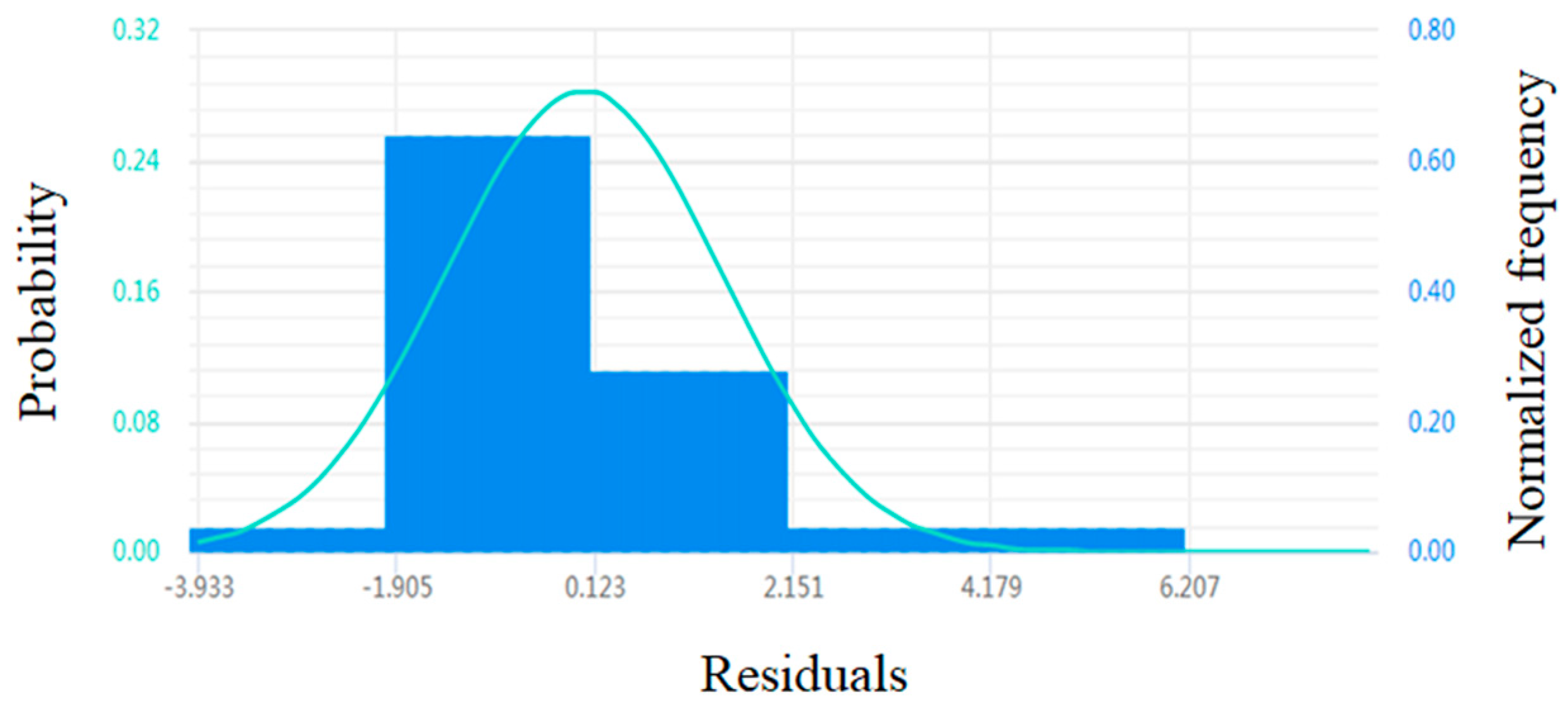
(3)

The residual term represents the difference between the observed value of each sample and the value estimated by the model. In general, the normal distribution is used to test the residual term: if the test residual data conform to the normal distribution, the model can be considered to be well constructed. Residual normality is used to test the reliability and periodicity of data based on experimental sample data. The analysis of residual normality is only one of the reliability test indices to test the stepwise regression model. To judge whether the regression model conforms to the standard, only the residual items need to meet the normal distribution intuitively. The residual values of regression analysis data in this paper conform to the normal distribution, indicating that the stepwise regression model is reasonable, as shown in Figure 19.

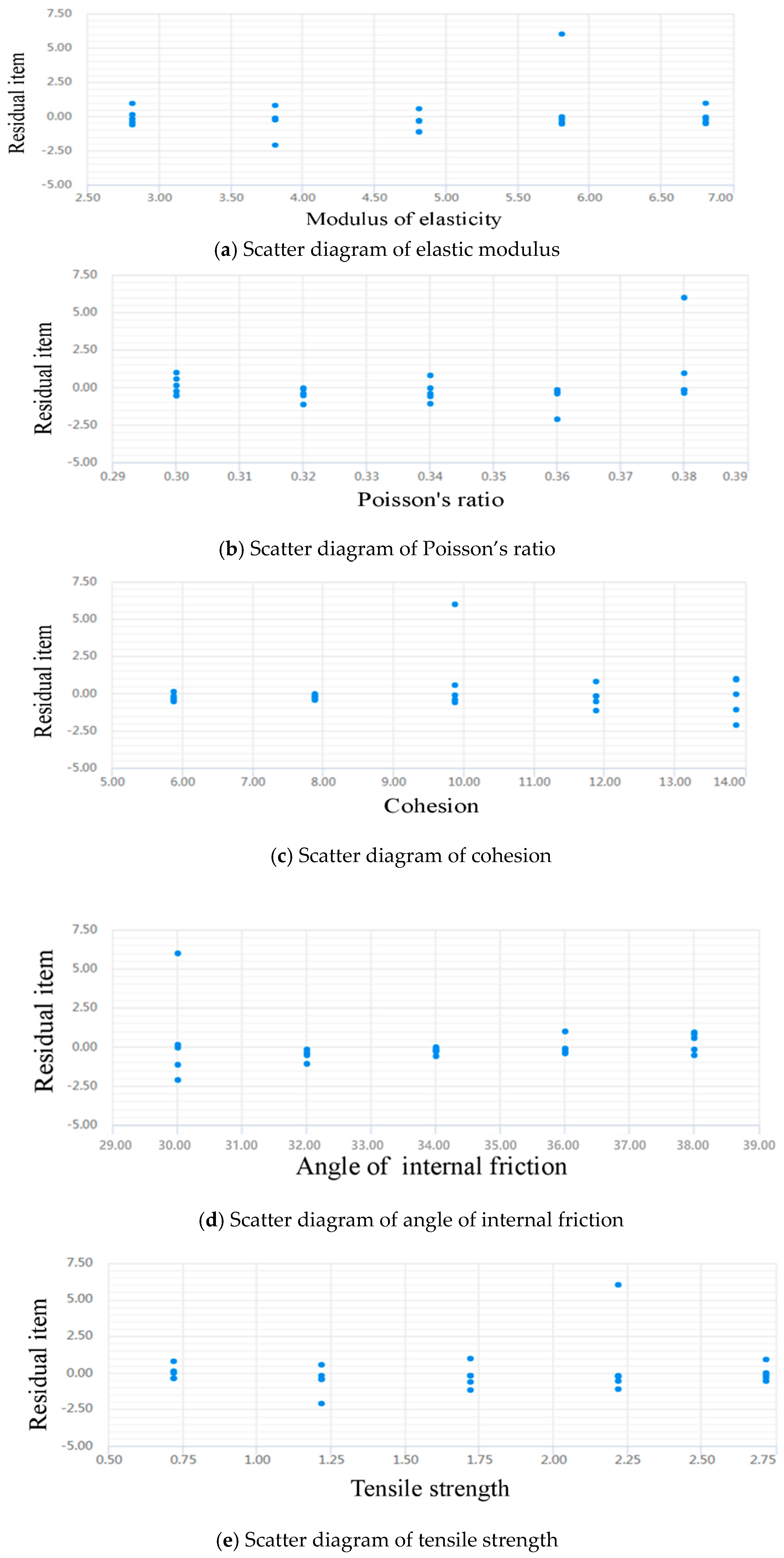
(4)

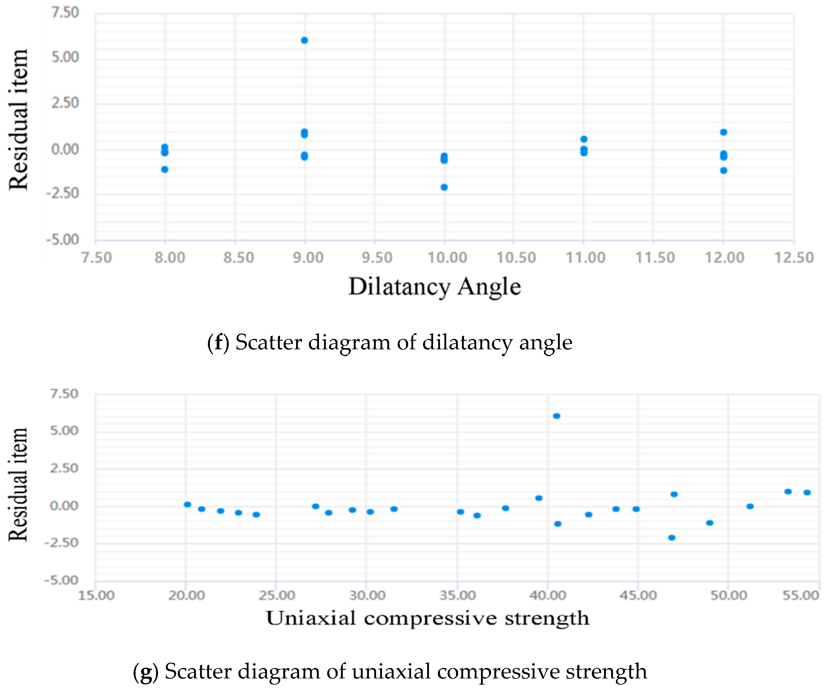
The heteroscedasticity was validated by plotting scatter diagram of the independent and dependent variables with the residual term. The heteroscedasticity can be compared to the variance: it is the difference in variance between the explaining variable that omitted from the model and the unimportant explained variable. Accordingly, to determine the heteroscedasticity, the data can be examined for signs of regularity in the corresponding scattered points. If the residual is notably increased or decreased with any increase in the independent variable, the regularity is obvious; then, the model has heteroscedasticity and its construction can be considered poor. All of the independent and dependent variables considered here were plotted in a scatter diagram, as shown in Figure 20.

The scatter diagrams in Figure 20a–g illustrate that the regression analysis data exhibit no regularity. When the independent variables are varied, the residual items do not exhibit regular increases or decreases. Therefore, there is no correlation between the residual items and related variables and no heteroscedasticity, indicating that the model is well constructed.

In summary, the independent variables C and Φ exhibit significant correlations with UCS. As indicated by the regression coefficients, these two independent variables have a positive relationship with UCS, which is in line with the results of the orthogonal experiment; the interpretation parameters are also considered to be optimal. In addition, test parameters such as multicollinearity, autocorrelation, residual normality and heteroscedasticity are also in line with the corresponding standards. Based on the principle of stepwise regression analysis, a regression model for UCS, C and Φ was established and a functional relationship between the main controlling parameters and UCS was determined as follows.

y = β₀ + β₁x₁ + β₂x₂

(8)

where y is UCS (MPa), x₁ is C (MPa), x₂ is Φ (in degrees) and the coefficients β₁ and β₂ indicate the degree of influence of the main controlling parameters on UCS.

According to the principle of stepwise regression analysis, the standardized coefficient of the regression model represents primarily the degree of influence of different independent variables on the dependent variable. It compares the relative importance of all influencing parameters on the dependent variable after nondimensionalization of the parameters, and the non-standardized coefficient should be used for actual prediction using the regression model. The final stepwise regression equation is as follows.

y = 3.628x₁ + 0.557x₂ − 18.059

(9)

4.2. Reliability Analysis of Stepwise Regression Equation of Coal Compressive Strength

To further verify the accuracy and adaptability of the stepwise regression in Equation (9) to the prediction of the UCS of coal seams, the mechanical parameters of coal seams such as Zhaolou (ZL), Baodian (BD), Huaheng (HH), Xinhe (XH) and Dongtan (DT) were used. The second regression equation (σ_c = 11.31 + 4.19x₁ − 0.017x₁², where x₁ is the elastic modulus) for predicting the UCS of the 11-2 coal roof rock in the Huainan mining area was compared and analyzed using the method previously described in [22]. The calculation results are shown in

Table 9. Prediction results of compressive strength of coal seams in different coal mines.

Coal Sample	E (GPa)	C (MPa)	Φ (°)	UCS (MPa)	Stepwise Regression		Quadratic Regression
					Predicted Value	Error	Predicted Value	Error
ZL3 coal seam	4.32	6.4	25.2	22.36	19.2	14.13%	29.09	30.1%
BD3 down coal seam	13.93	8.2	30.24	26.63	28.53	7.15%	66.38	149.36%
BD 3 coal seam	14.35	7.0	30	25.91	24.05	7.19%	67.94	162.20%
HH 3 coal seam	7.87	5.4	32.3	18.22	19.67	7.15%	43.23	137.28%
XH 3 coal seam	5.23	5.7	29.3	19.22	18.94	1.45%	32.76	70.44%
DT3 coal seam	3.97	5.64	31.5	19.6	19.95	1.78%	27.68	41.21%
DT 3 up coal seam	3.43	5.52	33	20.82	20.35	2.26%	25.48	22.39%
DT 3 down coal seam	3.8	6.5	33	24.04	23.9	0.57%	26.99	12.26%

.

According to the compressive strength values of different coal seams, the maximum error of the prediction results of a stepwise regression equation was seen for Zhaolou coal seam 3 (14.13%); the other prediction errors were less than 10%. The minimum error, of just 0.57%, was seen for 3_down coal seam of Dongtan coal mine. However, the error of the quadratic regression prediction results was large: the minimum error was 12.26%, and the maximum error was as high as 162.20%. It can be seen, therefore, that a secondary regression model of the compressive strength of roof strata is only suitable for predicting the UCS of coal seams with small elastic modulus, and it has large errors and poor universality. However, the stepwise regression prediction equation established in this study had the advantages of small errors, high accuracy and good universality.

5. Conclusions

(1)

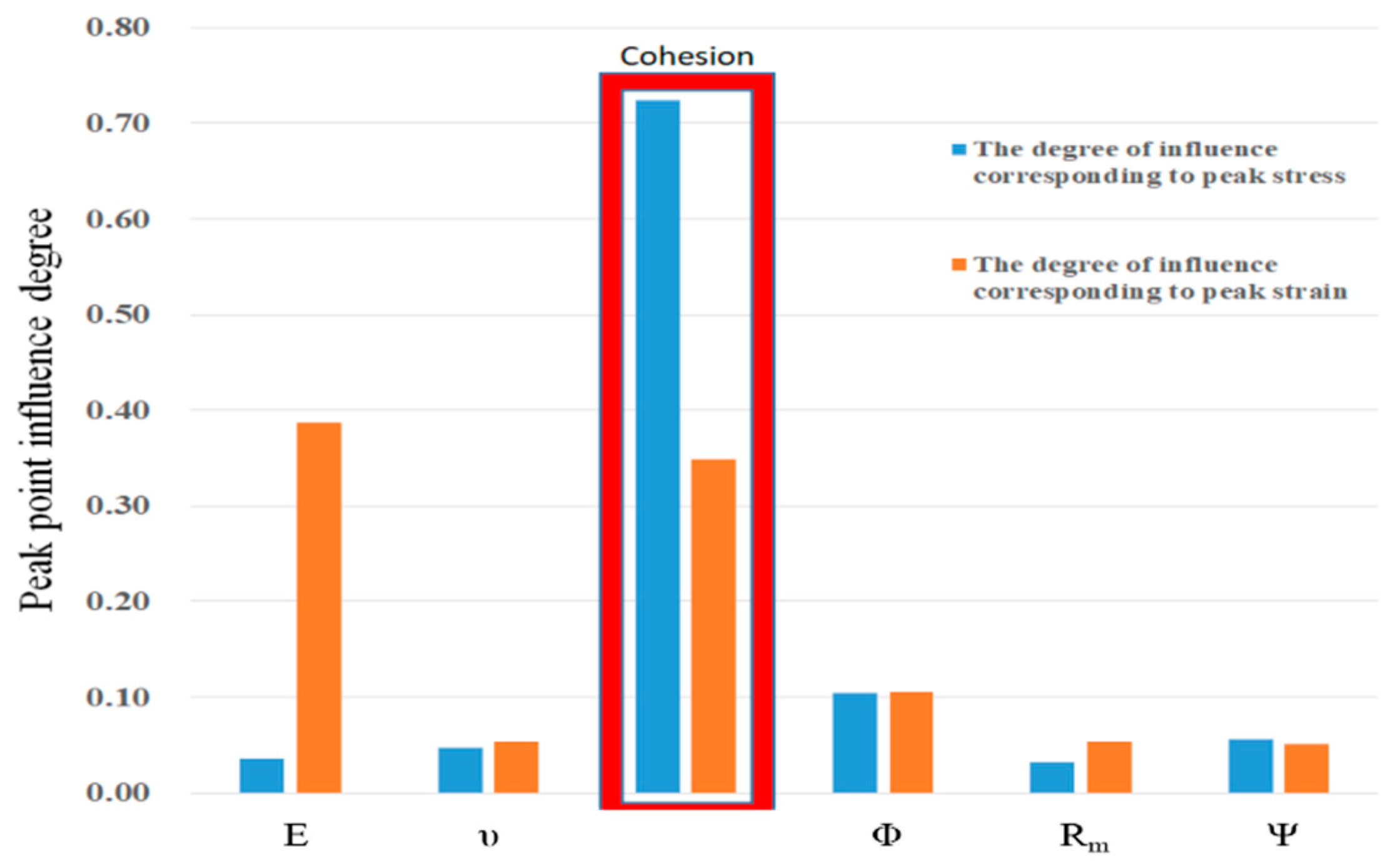
The degree of influence of mechanical parameters on UCS decreases in the following order: C > Φ > Ψ > υ > E > R_m. Thus, of these parameters, C has the greatest influence, followed by Φ. The other mechanical parameters considered have little influence on UCS for coal samples, and their relationships with UCS exhibit nonlinear characteristics. Thus, the main parameters controlling UCS are C and Φ.

(2)

Different mechanical parameters have different degrees of influence on PS, with degree of influence decreasing in the following order: E > C > Φ > R_m > υ > Ψ. Thus, E has the greatest influence on PS (negative linear relationship), followed by C (positive linear relationship). The other mechanical parameters considered have little influence on PS, and the main parameters controlling PS are E and C.

(3)

The degree of influence of mechanical parameters on peak strength has been determined based on an orthogonal simulation experiment, with the mechanical parameters without obvious significance being eliminated by a stepwise regression analysis model. The stepwise regression equation is a mathematical model with C and Φ as independent variables and UCS as a dependent variable, and the reliability of the regression prediction equation was verified. The prediction results have small error, high fitting degree and good adaptability, indicating that the model can realize the prediction of UCS.

The precision of the stepwise regression model depends on the number of test samples, which can be increased in the later stages of a design project to further improve the precision of the projection model.

References

1. Xie, H.P.; Peng, R.D.; Ju, Y. Energy dissipation of rock deformation and fracture. Chin. J. Rock Mech. Eng. 2004, 21, 3565–3570. [Google Scholar]
2. Wu, F.B. Experimental study on mechanical characteristics of mica quartz schist foliation surface. Chin. J. Geotech. Eng. 2019, 41 (Suppl. 1), 117–120. [Google Scholar]
3. Cao, W.G.; Zhang, C.; He, M.; Liu, T. Statistical damage simulation method of strain softening deformation process for rock considering characteristics of void compaction stage. Chin. J. Geotech. Eng. 2016, 10, 1754–1761. [Google Scholar]
4. Matin, S.S.; Farahzadi, L.; Makaremi, S.; Chelgani, S.C.; Sattari, G. Variable selection and prediction of uniaxial compressive strength and modulus of elasticity by random forest. Appl. Soft. Comput. 2018, 70, 980–987. [Google Scholar] [CrossRef]
5. Cheshomi, A.; Hajipour, G.; Hassanpour, J.; Dashtaki, B.B.; Firouzei, Y.; Sheshde, E.A. Estimation of uniaxial compressive strength of shale using indentation testing. J. Petrol. Sci. Eng. 2017, 151, 24–30. [Google Scholar] [CrossRef]
6. Qin, Q.C.; Li, K.G.; Yang, B.W.; Wang, T.; Zhang, X.Y.; Guo, W. Analysis of damage characteristics of key characteristic points in the whole stress-strain process of rock. Rock Soil Mech. 2018, 39, 14–24. [Google Scholar]
7. Chen, Y.L.; Zhang, Y.N.; Li, K.B.; Teng, J.Y. Distinct element numerical analysis of failure process of interlayered rock subjected to uniaxial compression. J. Min. Saf. Eng. 2017, 4, 795–802, 816. [Google Scholar]
8. Lei, S.; Kang, H.P.; Gao, F.Q.; Si, L.P. Study and application of a method for rapid-determination of uniaxial compressive strength of weak coal in Xinyuan coal mine. J. China Coal Soc. 2019, 44, 3412–3422. [Google Scholar]
9. Naji, A.M.; Emad, M.Z.; Rehman, H.; Yoo, H. Geological and geomechanical heterogeneity in deep hydropower tunnels: A rock burst failure case study. Tunn. Undergr. Space Technol. 2019, 84, 507–521. [Google Scholar] [CrossRef]
10. Li, A.; Shao, G.J.; Su, J.B.; Liu, J.C.; Sun, Y. Uniaxial compression test and numerical simulation for alternatively soft and hard interbedded rock mass. J. Hohai Univ. (Nat. Sci.) 2018, 6, 533–538. [Google Scholar]
11. Yesiloglu-Gultekin, N.; Gokceoglu, C.; Sezer, E.A. Prediction of uniaxial compressive strength of granitic rocks by various nonlinear tools and comparison of their performances. Int. J. Rock Mech. Min. 2013, 62, 113–122. [Google Scholar] [CrossRef]
12. Huang, Y.G.; Zhang, T.J. Plastic failure characteristics of deep roadway with high ground stress and grouting support. J. Min. Saf. Eng. 2019, 5, 949–958. [Google Scholar]
13. Si, X.F.; Gong, F.Q.; Li, X.B.; Wang, S.Y.; Luo, S. Dynamic Mohr–Coulomb and Hoek–Brown strength criteria of sandstone at high strain rates. Int. J. Rock Mech. Min. 2019, 115, 48–59. [Google Scholar] [CrossRef]
14. Wang, Q.; Sun, H.B.; Jiang, B.; Gao, S.; Li, S.C.; Gao, H.K. The method of predicting rock uniaxial compressive strength based on digital drilling and support vector machine. Rock Soil Mech. 2019, 40, 1221–1228. [Google Scholar]
15. Yang, X.; Meng, Y.F.; Li, G.; Wang, L.; Li, C. An empirical equation to estimate uniaxial compressive strength for anisotropic rocks. Rock Soil Mech. 2017, 9, 2611–2655. [Google Scholar]
16. Li, Y.W.; Jiang, Y.D.; Yang, Y.M.; Zhang, K.X.; Ren, Z.; Li, H.T.; Ma, Z.Q. Research on loading rate effect ofuniaxial compressive strength of coal. J. Min. Saf. Eng. 2016, 4, 754–760. [Google Scholar]
17. Chen, P.; Liu, C.Y.; Wang, Y.Y. Size effect on peak axial strain and stress-strain behavior of concrete subjected to axial compression. Constr. Build. Mater. 2018, 10, 645–655. [Google Scholar] [CrossRef]
18. Lu, G.D.; Yan, E.C.; Wang, H.L.; Wang, X.M.; Xie, L.F. Prediction on uniaxial compressive strength of carbonate based on geological nature of rock. J. Jilin Uni. (Earth. Sci. Ed) 2013, 6, 1915–1921+1935. [Google Scholar]
19. Palchik, V. Use of stress–strain model based on Haldane’s distribution function for prediction of elastic modulus. Int. J. Rock Mech. Min. 2007, 4, 514–524. [Google Scholar] [CrossRef]
20. Zhou, H.; Yang, Y.S.; Xiao, H.B.; Zhang, C.Q.; Fu, Y.P. Research on loading rate effect on tensile strength property on hard brittle marble-teat characteristics and mechanism. Chin. J. Rock Mech. Eng. 2013, 9, 1868–1875. [Google Scholar]
21. He, P.; Liu, C.W.; Wang, C.; You, S.; Wang, W.Q.; Li, L. Correlation analysis of uniaxial compressive strength and elastic modulus of sedimentary. J. Sichuan Univ. (Eng. Sci. Ed.) 2011, 4, 7–12. [Google Scholar]
22. Yang, K.; Yuan, L.; Qi, L.G.; Liao, B.C. Establishing predictive model for rock uniaxial compressive strengthon No.11-2 coal seam roof in Huainan mining area. Chin. J. Rock Mech. Eng. 2013, 10, 1991–1998. [Google Scholar]
23. Ashtari, M.; Mousavi, S.E.; Cheshomi, A.; Khamechian, M. Evaluation of the single compressive strength test in estimating uniaxial compressive and Brazilian tensile strengths and elastic modulus of marlstone. Eng. Geol. 2019, 248, 256–266. [Google Scholar] [CrossRef]
24. Qi, L.G.; Yang, K.; Lu, W.; Yan, S.Y. Statistical Analysis on Uniaxial Compressive Strength of Coal Measures. Coal Sci. Technol. 2013, 2, 100–103. [Google Scholar]
25. Lin, B.; Xu, D. Relationship between uniaxial compressive strength and elastic modulus of rocks based on different lithological characters. Saf. Coal Mines 2017, 3, 160–162, 166. [Google Scholar]
26. Hu, Y.X.; Liu, X.R.; Xu, H.; Ge, H. Multiple linear regression prediction models to predict the uniaxial compressive strength and the elastic modulus of Pengguan complex. Geotech. Investig. Surv. 2010, 12, 15–21. [Google Scholar]
27. Małkowski, P.; Ostrowski, Ł.; Brodny, J. Analysis of Young′s modulus for Carboniferous sedimentary rocks and its relationship with Uniaxial compressive strength using different methods of modulus determination. J. Sustain. Min. 2018, 3, 145–157. [Google Scholar] [CrossRef]
28. Hoek, E.; Brown, E.T. Practical estimates of rock mass strength. Int. J. Rock Mech. Min. 1997, 34, 1165–1186. [Google Scholar] [CrossRef]
29. Wang, S.L.; Yin, S.D.; Wu, Z.J. Strain-softening analysis of a spherical cavity. Int. J. Numer. Anal. Met. 2010, 36, 182–202. [Google Scholar] [CrossRef]
30. Vermeer, P.A.; Borst, R. Non-associated plasticity for soils. Concr. Rock Heron 1984, 29, 3–64. [Google Scholar]
31. Alejano, L.R.; Alonso, E. Considerations of the dilatancy angle in rocks and rock masses. Int. J. Rock Mech. Min. 2005, 42, 481–507. [Google Scholar] [CrossRef]
32. Shen, H.Z.; Wang, S.L.; Liu, Q.S. Simulation of constitutive curves for strain-softening rock in triaxial compression. Rock Soil Mech. 2014, 6, 1647–1654. [Google Scholar]
33. Meng, Q.B.; Han, L.J.; Qiao, W.G.; Lin, D.G.; Wei, L.C. Numerical simulation of crosssection shape optimizati-on design of deep soft rock roadway under high stress. J. Min. Saf. Eng. 2012, 5, 650–656. [Google Scholar]
34. Li, G.; Liang, B.; Zhang, G.H. Deformation Features of Roadway in Highly Stressed Soft Rock and Design of Supporting Parameters. J. Min. Saf. Eng. 2009, 2, 183–186. [Google Scholar]
35. Liu, J.; Zhao, G.Y.; Liang, W.Z.; Wu, H.; Peng, F.H. Numerical simulation of uniaxial compressive strength and failure characteristics in nonuniform rock materials. Rock Soil Mech. 2018, 39 (Suppl. 1), 505–512. [Google Scholar]
36. Zhou, A.Z.; Lu, T.H. Elasto-plastic constitutive model of soil-structure interface in consideration of strain softening and dilation. Acta Mech. Solida Sin. 2009, 2, 171–179. [Google Scholar] [CrossRef]
37. He, Z.M.; Peng, Z.B.; Cao, P.; Zhou, L.J. Test and numerical simulation for stratified rock mass under uniaxial compression. J. Cent. South Univ. (Sci. Technol.) 2010, 5, 1906–1912. [Google Scholar]
38. Shen, P.W.; Tang, H.M.; Ning, Y.B.; Xia, D. A damage mechanics based on the constitutive model for strain softening rocks. Eng. Fract. Mech. 2019, 216, 106521. [Google Scholar] [CrossRef]
39. Itasca Consulting Group Inc. Fast Lagrangian Analysis of Continua in 3 Dimensions User’s Guide; Section 3.6, Chioce of Constitutive Model, 3-71-3-80; Itasca Consulting Group Inc.: Minneapolis, MN, USA, 2005. [Google Scholar]
40. Zhou, Y.; Wang, T.; Lv, Q.; Zhu, Y.L.; Wang, X.X. Study on strain softening model of rock based on FLAC3D. J. Yangtze River Sci. Res. Inst. 2012, 5, 51–56, 61. [Google Scholar]
41. Zhang, W.; Ma, Q.Y. Performance analysis on compressive strength and splitting tensile strength of the Nano-silica modified shringkage-compensating concrete under sulfate erosion. China Concrete. Cem. Prod. 2013, 12, 13–16. [Google Scholar]
42. Wang, K.; Diao, X.H.; Lai, J.Y.; Huang, G.L. Engineering application comparison of strain softening model and Mohr-Columb model in FLAC3D. China Sci. 2015, 1, 55–59, 69. [Google Scholar]
43. Yang, S.J.; Zeng, S.; Wang, H.L. Experimental study on mechanical effect of loading rate on limestone. Chin. J. Geotech. Eng. 2005, 7, 786–788. [Google Scholar]
44. Li, W.; Tan, Z.Y. Prediction of uniaxial compressive strength of rock based on P-wave modulus. Rock Soil Mech. 2016, 37, 381–387. [Google Scholar]
45. Zhao, Z.L.; Zhao, K.; Wang, X. Study on mechanical properties and damage evolution of coal-like rocks under different loading rates. Coal Sci. Technol. 2017, 10, 41–47. [Google Scholar]
46. Zhao, B.C.; He, S.L.; Lu, X.X. Analysis on Influence Factors of Surface Subsidence in Shallow Coal Seam Mining. Min. Saf. Environ. Prot. 2019, 4, 104–107, 112. [Google Scholar]
47. Liu, X.R.; Yang, S.Q. Numerical study of rock micromechanics parameters based on orthogonal test. J. Basic. Sci. Eng. 2018, 4, 918–928. [Google Scholar]
48. Gao, F.Q.; Wang, X.K. Orthogonal numerical simulation on sensitivity of rock mechanical parameters. J. Min. Saf. Eng. 2008, 1, 95–98. [Google Scholar]
49. Zhao, G.Z.; Ma, Z.G.; Zhu, Q.H.; Mao, X.B.; Feng, M.M. Roadway deformation during riding mining in soft rock. Int. J. Min. Sci. Technol. 2012, 4, 539–544. [Google Scholar] [CrossRef]
50. Li, S.C.; Wang, Q.; Wang, H.T.; Jiang, B.; Wang, D.C.; Zhang, B.; Li, Y.; Ruan, Q. Model test study on surrounding rock deformation and failure mechanisms of deep roadways with thick top coal. Tunn. Undergr. Space Technol. 2015, 47, 52–63. [Google Scholar] [CrossRef]
Figure 1. Technical workflow.
Energies 13 03640 g001
Figure 2. Coal samples as prepared for experiment.
Energies 13 03640 g002
Figure 3. RMT-150B servo-control testing machine.
Energies 13 03640 g003
Figure 4. Specimen loading diagram: ① upper bearing plate; ② axial displacement sensor gripper; ③ transverse displacement sensor; ④ transverse displacement sensor mounting seat; ⑤ axial displacement sensor; ⑥ sample; ⑦ sensor mounting plate; ⑧ lower bearing plate; ⑨ bearing seat ⑩ locating pin; ⑪ adjustment plate; ⑫ foundation support; ⑬ baseboard; and ⑭ located block.
Energies 13 03640 g004
Figure 5. Failure pattern of coal samples.
Energies 13 03640 g005
Figure 6. Experimental curve of mechanics.
Energies 13 03640 g006
Figure 7. Mesh generation and boundary conditions of the computational model.
Energies 13 03640 g007
Figure 8. Stress–strain curves for different shape models.
Energies 13 03640 g008
Figure 9. Comparison of numerical simulation results under different cell mesh sizes.
Energies 13 03640 g009
Figure 10. Stress–strain curves for different loading rates.
Energies 13 03640 g010
Figure 11. Orthogonal experimental design flow.
Energies 13 03640 g011
Figure 12. Effect of various parameters on changes in rock compressive strength.
Energies 13 03640 g012aEnergies 13 03640 g012b
Figure 13. Whole stress–strain process curve.
Energies 13 03640 g013
Figure 14. Influence of variation in each parameter on peak strain sensitivity.
Energies 13 03640 g014
Figure 15. Influence degree of cohesion on peak strain under different elastic modulus conditions.
Energies 13 03640 g015
Figure 16. Histogram of the influence of mechanical parameters on peak stress and strain.
Energies 13 03640 g016
Figure 17. Predictive regression analysis technical workflow.
Energies 13 03640 g017
Figure 18. Correlation test of regression model.
Energies 13 03640 g018
Figure 19. Normal distribution of residual data.
Energies 13 03640 g019
Figure 20. Scatter diagram of related variables and residuals in the regression model.
Energies 13 03640 g020aEnergies 13 03640 g020b