Abstract
With an increasing share of renewable energy resources participating in electricity markets, there is a growing dependence between renewable power production and clearing prices of spot markets. Modeling this dependence using bivariate analysis can result in underestimation of market risks and adverse effects for stakeholders’ risk management. To enable an undistorted risk assessment, we are using a copula approach to precisely and jointly model electricity prices and infeed volumes of wind power. We simulate the case of wind farm operators using power purchase agreements (PPAs) to shift the price risk to an energy trader, who integrates the infeed into its portfolio. The trader’s portfolio can either be geographically dispersed, or highly localized. Based on its portfolio, the energy trader can decide to use derivatives such as futures to manage its risk exposure. The trader decides on future volumes subject to its portfolio’s inherent volatility. With a given risk averse strategy, a sufficiently diverse portfolio can help reduce the necessity to trade futures and subsequently the disadvantage of having to pay potential risk premiums.
Keywords:
portfolio; portfolio management; risk; risk assessment; energy trading; power purchase agreements; PPA; copula 1. Introduction
In Germany, as in many other countries, market penetration of volatile renewable electricity producers has reached a significant level. In accordance to federal government and European Union goals, the German power sector is set to increase its share of electricity produced by renewable energy sources (RES) to at least 35% by the end of 2020, at least 65% in 2030, and at least 80% in 2050 [1]. RES in this context are wind, solar, biomass, hydro and niche producers (e.g., geothermal). The share of RES in the gross electricity consumption reached 31.6% in 2016, double the share compared to 2008 [2]. This puts it on track to reach the stated goal. Because of the volatile nature of renewable production, the doubling of produced electricity was accompanied with a bigger increase in production capacity of 287%, corresponding to a share of the total production capacity of 52% [3].
The increase in renewable energy generation is primarily driven by expansion of wind and solar power. This expansion of volatile electricity production has measurable effects on price volatility and dependencies between renewable infeed and prices [4,5]. A principle component analysis (PCA) of price variation shows that seasonal factors, which affect renewable generation, are a major component [6]. A similar approach has been used to assess the role of prices spikes in electricity markets [7]. The volatility caused by RES expansion poses numerous challenges for actors in the energy system. Potential investors in new power plants need their assets to generate enough revenue to cover fixed costs; policy makers have to ensure that energy demand can (almost) always be satisfied. These challenges can be tackled in numerous ways. New market designs can help to ensure matching of supply and demand [8,9], and advanced algorithmic techniques can be used to automate trading in energy markets [10,11]. Our work falls in the realm of statistical modelling that allows for advanced forecasting in the highly stochastic energy system.
There is a large body of work in statistical modelling of energy systems and markets, respectively. Using a GARCH (Generalized Autoregressive Conditional Heteroskedasticity) model, [4] shows that wind power decreases the average price level, but increases volatility. The same relationship is shown by [12]. This effect is not only present in the German energy system, but has also been demonstrated for the Texan electricity market [13]. Electricity prices further inhibit statistically significant calendar effects [14]. While most renewable energy producers are currently shielded from these market effects by guaranteed infeed tariffs, this system is being phased out gradually in Germany. New plants do not get guaranteed remuneration for their infeed and old plants are dropping out of the compensation scheme. As a consequence of the shift from guaranteed infeed tariffs to market-based remuneration, there is a trend to market-based financing mechanisms for new installations and plants without fixed compensation. One of these are power purchase agreements (PPAs). Here, the production of a specific electricity producer is sold to an energy trading company or directly to a consumer. While there is a large potential for increasing use of PPAs, risk averse energy trading companies have to manage the acquired risk exposure. The underlying drivers to motivate risk aversion are diverse among different actors. Asset owners are typically risk averse because they carry the capital costs for new installations. To securely refinance their investment, they need to hedge against risks from regulation and technical failure [15]. In liberalized energy markets they also have to hedge against market risks. A common aspect of this risk for different actors along the energy value chain is the aforementioned problem of joint price and quantity risk. The seminal paper of [16] describes this problem for farmers wishing to protect themselves from output uncertainty and unknown market prices. Not only is the future production of a volatile (e.g., wind) portfolio unknown, the revenue from this production is also unclear. The adverse relationship of production and prices, i.e., lower prices in situations with high production and vice versa, exposes market actors to a higher risk than the two individual risk factors [17,18]. This also makes it risky to perform a simple volume hedge, where the hedged quantity is the expected production volume. Due to the dependence structure, this strategy would leave the market actor exposed to disregarded risk aspects.
Owners of RES regularly conclude agreements with market access providers, who offer them so PPAs in the form of “fixed-for-fluctuating-agreements”, where the owner receives a fixed price for the future production and thus remains solely with the volumetric risk [19]. As the production volume is driven by weather phenomena, it can be assessed by project developers without in-depth knowledge of energy markets. Companies offering “fixed-for-fluctuating-agreements” or power purchase agreements (PPAs) are paying the producer fixed rates, while facing both unknown production volumes and market prices in the future. They are therefore motivated to hedge against both price and volumetric risks using different instruments. As prices and generation are both stochastic and cross-correlated, this is a complex task. A hedging decision which does not take the stochastic relationship of quantities and price into account risks undervaluing the situations with the highest negative impact on revenue.
Financial risks (not only in energy markets) are often quantified by the Value-at-Risk (VaR) metric. It describes the highest possible loss of a return distribution with a confidence, where p is the exogenously defined risk level [20]. Typical VaR levels are 5% (e.g., [21]) or 1% (e.g., [22]). An extension is Conditional Value-at-Risk (CVaR), which conditions VaR on information before a specific point in time [23]. A second measure common to risk management is Expected Shortfall (ES). It is the expected value of the Value-at-Risk at the confidence level. Expected Shortfall is better suited to conceptualize the risk for fat-tailed return distributions, because it reflects the resulting higher likelihood of extreme values in its value [24].
To optimize its market position, an energy trader has to model the dependence structure of production and prices accounting for its complexity, especially with regard to the joint distribution’s tails. This work focuses on modeling this aspect with regard to the wholesale electricity market, as participation of volatile renewable energy sources in other markets (e.g., regulation) is uncommon in Germany. A mathematical tool to do so are copulas (see, e.g., [24]). Copulas disentangle the dependence structure of multiple variables from their marginal distributions. They are regularly used in applications of mathematical finance and economics, but gained interest in energy research in the past years [25,26]. With the combination of fitted marginal models and copulas, market prices and infeed volumes under a joint distribution can be simulated. The resulting values can be used to optimize the hedging decision using different hedging instruments and to reduce the risk an energy trading company faces. The process of the market position optimization is similar to the work of [19], who used the approach in an analysis of the Danish energy market. Using German data, we develop a better understanding of the relationship of wind power infeed and prices in this market. The final risk model assumes futures prices that equal the expected wholesale price, i.e., it assumes efficient (financial) markets. Doing so is common practice (see, e.g., [18,19,21]). This approach enables a focus on the variance effects of different hedging instruments, rather than expected revenue, for dealing with the price risk.
The remainder of this paper is structured as follows. First, data and the distribution function estimation process are presented. Then, the estimated distribution functions are used to bootstrap a simulation of joint infeed and price realizations. Using this simulation, different portfolios are optimized with regard to the remaining variance in revenues. The estimation and simulation procedure can be summarized by the following steps:
- Apply outlier model to price data;
- Apply logit-transform to infeed data;
- Estimate seasonal models;
- Estimate autoregressive and moving average components and variance terms;
- Estimate suitable distributions for the standardized residuals;
- Estimate suitable copula.
With the fitted model, Monte Carlo simulations can be performed:
- Draw random samples from copula;
- Re-transform these to price and infeed values for a chosen time-period;
- Estimate values of hedging instruments for different portfolios;
- Minimize variance of revenue distribution over different quantities of hedging contracts for different portfolios.
Using this approach, we show that a copula based variance minimizing hedge can reduce Conditional Value-at-Risk (CVaR) of a wind power portfolio significantly and improve with regard to expected shortfall (ES) compared to a simpler volume hedge (based on the expected production). Further, we build a variance reduced portfolio and show that needed hedging volumes are lower for both volume hedge und variance minimizing hedge. Our contribution is thus two-fold. First, we provide a statistical analysis of the complex joint relationship of wind power infeed and electricity prices in the German market. Second, we develop an initial set of tools for risk management of volatile portfolios in electricity markets with high RES penetration.
2. Data
The historical price data and wind infeed (min-max normalized) can be seen in Figure 1. Price data is based on German day-ahead clearing prices of EPEX SPOT (https://www.epexspot.com/en). While there are other marketplaces for electricity, and a large volume of over-the-counter (OTC) trading outside energy exchanges, the day-ahead auction is the exchange-based marketplace with highest liquidity in Germany. The original resolution of our data is EUR/MWh. While seemingly counter-intuitive for the analysis of volatility, it is common practice to aggregate the data to daily values. The main reason is that the day-ahead auction clears for all hourly slots of the next day simultaneously. Because of this, the prices of the day-ahead auction do not constitute a sequential series [27,28,29].
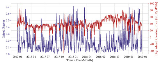
Figure 1.
German wind infeed and Day Ahead spot prices from 2017 until spring 2019. Infeed is scaled as a factor of total available capacity. Periods of common high volatility are recognizable.
Part of the wind portfolio of Next Kraftwerke (https://www.next-kraftwerke.com/) constitutes the data source for wind power infeed. The portfolio is preprocessed such that data of 46 wind power plants for a time span of 820 days between January 2017 and March 2019 is available. It has a linear correlation coefficient of with the total German wind power infeed, meaning it is highly representative for the German geographic properties. The infeed is processed using two transformations. As it has an upward trend due to increasing installed capacity, it is standardized as a factor of the total installed capacity. Then, a logistic transformation is applied to the standardized time series. This is due to the fact that boundaries are problematic when modeling the mean and variance models [19]. Before fitting the models, the mean value is subtracted from the time series of wind and prices, i.e., they are centered.
Figure 2 shows the joint distribution of the infeed factor (as average across the portfolio) and the spot prices as well as the joint distribution of the transformed time series. A clear dependency is visible. The descriptive statistics in Table 1 confirm the visual analysis.
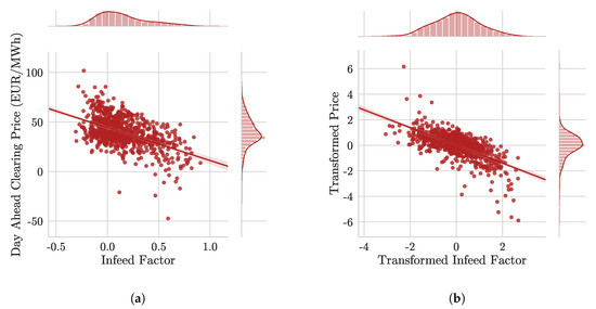
Figure 2.
Empirical distribution of wind infeed and electricity wholesale day-ahead prices. (a) Original infeed and price data; (b) Infeed and prices after transformation with the marginal models (see also Section 3).

Table 1.
Descriptive statistics for the empirical infeed and price time-series from 2017–2019.
Outliers and Seasonality
There are extreme spikes in electricity prices with a variety of methods to correct or replace these values [7,27,30]. Although extreme prices are correct data points, reflecting actual (if rare) economic regimes (cf. [31]), it is reasonable and common practice to treat the data when estimating stochastic models on it. This is because they disproportionately skew the time series [27,30]. This is especially true for hourly data that is more volatile than daily data, and also holds for the aggregated time series.
A simple method to treat extreme values is the fixed price threshold, where the time series is truncated subject to an upper and a lower bound. This method, amongst other similar ones, risks capturing either too few or too many outliers when dealing with data over a long time span. This due to the fact that electricity prices show strong mean variations of several years. An approach to tackle this issue is to remove the trend from the price data using a moving average before applying a filter to the residuals. Because the data not only varies in its mean but also in its variance, a variable price threshold of at least three standard deviations can be used. With some model extensions, this filter can be run iteratively until no more outliers are detected [30]. As the infeed is standardized on a -interval, no extreme values are present in the data. The preprocessing and choice of infeed data ensures that sufficiently long time spans with complete infeed data are available for all regarded power plants and no methods for interpolation of results are necessary.
An idiosyncratic aspect of electricity prices is their strong seasonal variation. To account for seasonality, we decompose the electricity price into three distinct components, a short-term and a long-term seasonal component (STSC and LTSC), and a stochastic component . Thus, the random variable representing the day-ahead price can be described as follows.
The LTSC is defined as a sinusoidal with a yearly period.
Parameters and determine phase and amplitude of the sinusoidal, whereas determines mean. The denominator is due to the fact that daily data is used.
The STSC , representing daily patterns, is not modeled as a sinusoidal with higher frequency, but using a least squares dummy variable approach. This is due to the fact that daily electricity consumption (and hence, price) patterns do not follow a smooth trend, but are subject to distinct difference between days, e.g., Sunday and Monday. Hence, daily dummy variables are assigned to each day of the week.
The days of the week are defined by , with the being Monday. denotes the length of one week in days, i.e., . denotes the parameter for day i. For instance, means that the short-term seasonal component for Mondays equals 1. Note that the random infeed quantity at time t can be modeled similarly to , however, there is no STSC as wind power does not follow a weekly pattern.
3. Estimation Procedure
The preprocessed data is used to estimate both marginal and joint distribution models. The widely used choice for the estimation of the marginal distribution are ARMA-GARCH models, which model the conditional mean and variance of the variables [4,6,19,24]. ARMA models describe stationary stochastic processes through autoregressive and moving-average terms. The autoregressive term uses p lags of the dependent variable and the moving-average term q lags of the error term. The errors are assumed to be independent and identically distributed (iid) and , where is usually the Normal distribution. The ARMA process for a random variable is
where and are the coefficients of the respective lag orders i and j. The GARCH extension replaces the error term with another autoregressive function to account for heteroskedasticity in the errors. It is also defined with a lag order of p and q and can be written as
where and are the coefficients of the respective lag orders i and j. The parameters are restricted to ensure stationarity, with , , , and [32]. Usually, . The normality condition can be relaxed, so that [21]. This not only permits more general parametric distributions for the error term, its distribution is also conditioned on its past. The conditioning on includes past information not only from the variable in question but from all variables. In many cases, when there is no cross-dependency, this can be restricted to the respective variable while still ensuring that all models are conditioned using the same information [24]. While the mean and variance models are coupled through the error term, they can be estimated separately, with the residuals of the ARMA model serving as input for the GARCH model [27]. This adds modeling flexibility and eases convergence. The lag order of the ARMA and GARCH models can be identified by comparing the Bayesian Information Criteria (BIC) or Akaike Information Criteria (AIC). The more widely used (e.g., [21,24]) BIC is defined as
where denotes the likelihood function. BIC penalizes model complextiy depending on model size (number of lag parameters) d and sample size n to avoid overfitting [27]. The model with the lowest BIC is considered best. After successfully estimating a model for both mean and variance, standardized residuals can be obtained. These are then used to estimate the copula. Also, a suitable distribution is fitted on the residuals to re-transform the samples obtained from the copula [24].
3.1. Goodness of Fit
The goodness of fit (GoF) of ARMA and GARCH models can be evaluated by plotting the (partial) autocorrelation functions ((P)ACF) of the model’s residuals. If the model is fitted well, no significant autocorrelation should remain. This can be tested using the Ljung-Box Q-test of serial independence. The test statistic is given by
Here, n is the sample size, the sample autocorrelation at lag k, and h the maximum length for which the test is being performed [33]. Under , the data is independently distributed. Thus, the test should not reject for the mean and variance model. Two widely used tests exist to evaluate the goodness of fit for the distributions which were estimated from the residuals. These are the Kolmogorov-Smirnov (KS) and Cramer-von-Mises (CvM) tests. Both are performed on the values of the residuals’ empirical CDF and test the similarity with a known (specified) distribution, where both are the same under :
is obtained using the empirical CDF and using the fitted parametric distribution. As KS and CvM tests are also available to evaluate the GoF of the copula model, subscript i denotes the applicability to the individual models.
3.2. Copula Model
Copulas are used to model the dependence structure of random variables [34]. Whereas, e.g., multivariate normal distributions require all variables and their dependency to have a normal distribution, copulas allow modeling separate marginal distributions of multiple random variables and their dependence. This allows for high flexibility in choosing a suitable distribution and simplifies the estimation procedure, as it can be done in stages [24]. Copulas are common in risk management and econometric applications [35,36,37,38]. A d-dimensional copula is a cumulative distribution function on d uniform marginals [39].
Then, with , three properties define a copula: 1) is non-decreasing in every component . 2) The marginal in component i can be obtained with for all because of its uniform distribution 3) When , is always non-negative. Assuming differentiability of the marginal distributions, the copula can be written as (see, e.g., [24])
Extensions of copula theory with regard to conditional distributions exist [40] and have been applied to energy modelling [21]. Consider for the bivariate case two random variables with a joint conditional distribution function and respective conditional marginal distribution functions . Then, a conditional copula with two dimensions exists, such that
Note that both the marginal models and the copula are conditioned on the past. If the marginals are continuous, the copula C is unique.
with . Each has the probability integral transform variable
The two main families of copulas are called Elliptical and Archimedean. Elliptical copulas are based on elliptical distributions, the two best-known of which are the Gaussian (normal) and Student’s t distribution. They are distinct in that the linear correlation fully describes their dependence structure (in contrast to other copula families, where this is false) [39]. In contrast to Elliptical copulas, Archimedean copulas are explicitly defined with so-called generator functions . They interpolate between dependence structures like independence and comonotonicity, typically using a free parameter . The general generator function is continuous and strictly decreasing: , with . In the bivariate case, the copula then has the form
Five different copula types have been fitted for the residuals. See Table 2 for their respective formulations. Which copula type is suitable for modeling can be evaluated using measures of dependence and goodness of fit tests.
Table 2.
Investigated copula types and mathematical formulations.
Goodness of Fit
Model specification and goodness of fit (GoF) tests can be seen as complementary. GoF tests can be limited in their explanatory power and be too weak or too strict to conclude a models suitability. Model specification tests are a good way to compare different models but do not always help in deciding the validity of a chosen model [24]. For fully parametric models, both the distributions resulting from the marginal models and the copula model are parametric. While this allows to fully specify a log-likelihood for estimation, the commonly used approach is to estimate a model in stages. In that case, the marginal models should not exhibit cross-equation restrictions. For nested models (e.g., comparing a Gaussian copula with a Student’s t copula) a likelihood ratio test can be used. An even simpler but very crude method is to rank the model likelihoods (see, e.g., [24]).
The KS and CvM test are two widely used GoF measures to compare an estimated copula with the empirical results. Their statistics adapted to the copula case are
and use the empirical copula which is defined as
As these tests are based on the empirical copula, they only work for constant, i.e., not time-dependent, copula models [24].
4. Estimation and Simulation Results
4.1. Aggregate Portfolio
4.1.1. Marginal Models
The estimation pipeline for the marginal models and the joint distribution using the copula are now applied to the portfolio of 46 wind power plants. The best fitting model combination is used to bootstrap a Monte Carlo simulation of possible scenarios. Table 3 shows the estimation of the marginal models for both the infeed and prices.
Table 3.
Estimates for model parameters, goodness of fit measures, and distribution of standardized residuals for infeed and price data. Italic typeset denotes parameters that are not highly significant. refers to Monday. The LB test subscripts indicate the lag. For the variance model, the squared residuals are tested.
Almost all parameters are significant. The insignificant parameters (marked by italic font) have all p-values under . Some typical characteristics of electricity markets are visible in the parameters, especially daily patterns. While weekdays (except Monday) have almost identical dummy factors, Saturday and especially Sunday have highly negative dummy parameters, due to the fact that reduced electricity consumption drives prices down.
The infeed data are logit-transformed and de-meaned. Then, a sinusoidal model is applied to account for intra-yearly seasonality. After considering the BIC of prospective lag orders, an ARMA(1,1) model is chosen for the autoregressive process. No significant heteroskedasticity is left in the residuals, which is confirmed with the Ljung-Box test on the squared residuals. Therefore, no GARCH model needs to be estimated. The standardized residuals are fitted to a normal distribution, after comparing the results of the KS and CvM tests to the skew normal distribution. Similar to the infeed, the price data is also de-meaned. Before applying the seasonal models, outliers are filtered with the approach described earlier and a threshold of four standard deviations. Subsequently, a sinusoidal long-term seasonal component and a dummy-based short-term seasonal component with dummies for each weekday are fitted. While the analysis of ACF/PACF plots makes a seasonal model likely, comparing the respective BIC values suggest a simple ARMA(2,2) process. Because the residuals show clear signs of heteroskedasticity, a GARCH(1,1) model is applied to them. A skew Student’s t distribution is then fitted to the standardized residuals.
After the marginal models are applied, the resulting standardized residual series exhibit a Spearman’s rank correlation of . This can be attributed to the marginal models stripping away independent properties inherent to the two time series. Further, it shows that the correlation of prices and infeed are not (only) due to seasonal effects explaining both price and infeed variations but due to their direct relationship. This result corresponds to the literature [41]. The residuals are transformed to uniformly distributed variables using the empirical CDF. With the resulting residuals, a copula can be estimated.
4.1.2. Copula Model
Different copula specifications and their estimates are shown in Table 4. The Frank and the Gumbel copula converged to the Independence copula, an unlikely outcome, and are therefore excluded. The best-performing was the Student’s t copula, although only marginally better than the Gaussian copula. As was shown in Figure 2b, the residuals of the marginal models for both infeed and prices show close resemblance to Gaussian characteristic. Still, the Student’s t copula demonstrates superiority with respect to all relevant GoF measures. It is therefore the most suitable candidate to bootstrap the simulations.
Table 4.
Estimates, log likelihoods, BIC and p-values of the KS- and CvM tests for different copula families estimated on standardized residuals. The copula with the lowest BIC is marked bold.
The student’s t copula requires symmetric dependency. Therefore, quantile dependence test is carried out (see Figure 3). The test shows a slight asymmetry in the dependency. The chosen copula is retained however, because the comparison of different copula families yields worse results for possible asymmetric copulas. Also, the empirical results are well within the 95% confidence intervals of a bootstrap simulation of the estimated Student’s t copula (Performed with ).
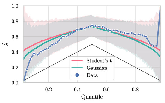
Figure 3.
Quantile dependence of the estimated copulas, together with corresponding 95% confidence intervals (depicted as shaded areas).
4.1.3. Simulation and Optimized Hedging
Based on the simulation framework, a routine for determination of the optimal hedging position is developed. In this scenario, the electricity trader’s goal is to minimize variance of its returns. As common in power purchase agreements, the trader is obligated to pay a fixed amount per unit of energy to the producer, no matter the time of feed-in. With this, the daily revenue of the traders’ portfolio can be calculated as
Here, denotes the (stochastic) infeed at time t, with being the first hour of day d. is the stochastic day-ahead price at time t. c is a capacity factor denoting the size of the portfolio to scale the revenue. The optimization routine is, however, scale invariant. Prices are aggregated per day, hence a factor of 24 is included in the expression. Again, this is barely for scaling, but does not affect the optimization procedure. Balancing risk is excluded in our analysis by assuming that the quantities sold on the day ahead market reflect the actual infeed, or . This is done for simplicity and because the issues arising from explicitly modelling balancing risk would call for a detailed explicit consideration and would aggravate assessment of the effect of the hedging position.
Following [19], we are imposing revenue neutral financial instruments. Doing so is common practice (cf. [18,19,21,42]) and enables a focus on the variance effects of hedging instruments in dealing with the price risk. The fair value of is then given by
is the risk-neutral measure. Under the rational expectation hypothesis it can be set equal to the physical measure , which accounts for the uncertainty arising from using historical data for the model (cf. [42,43]). Due to their liquidity, we are focusing on daily futures as hedging instruments. The payoff for one futures contract for day d is
with the price of the future at being [19]. The price of the future can be defined as the conditional spot price expectation [44,45]. When multiple hedging instruments are used, their payoff can be calculated as a linear combination of the individual contracts, . The total revenue is then
Enabling the optimization of the hedging position based on these calculations requires assumptions regarding the financial aspects of the given energy market. Under the rational expectation hypothesis, the expected revenue becomes . It is, however, not realistic [46,47], due to incompleteness of the electricity market. Still, it is common practice [17,21,43], therefore we proceed the same way. Further, we are setting the interest rate to zero, allowing for the optimization after simulating from the dependency model (cf. [19]). Because hedging is assumed to take place at time , the optimization is limited to a static hedge (in contrast to a dynamic hedge, where the hedged quantities can be dynamically altered after .) Furthermore, as [18] concede, the problem of timing, i.e., at which to perform hedging for a contract covering d, is complicated. This renders excluding it from the problem a reasonable option. An example of a model which includes the timing decision can be found in [48].
Since applying all assumptions to calculating prices for hedging instruments means that they are revenue-neutral as well, the optimization problem is reduced to the variance aspect, which can be formulated as
where n specifies the corresponding hedging instrument out of N different ones. With the corresponding quantities for each hedging instrument and for an arbitrary portfolio size, the CVaR and ES of the minimal variance hedge can be evaluated and compared. We are focusing on 2 exemplary months within our dataset, February and August. Both have different characteristics regarding wind infeed and price behavior. Portfolio size is normalized to a capacity of 100 MW. Table 5 shows the results for the total portfolio.
Table 5.
Risk assessment for the overall portfolio with and without hedging. Both hedging methods reduce variance and CVaR significantly, with the minimal variance hedge outperforming the volume hedge with respect to expected shortfall.
It can be seen that both hedging variants, the simple volume hedge and the variance minimization significantly reduce the CVaR. As is expected, the variance is reduced more strongly for the hedging method defining this as its goal. Interestingly, CVaR is reduced more strongly using the volume hedge. However, expected shortfall is reduced more under the variance minimizing hedging scheme. This means that while a volume hedge reduces the starting point of the revenue distribution’s tail more, the mass of the tail is reduced further under the variance minimizing hedge.
4.2. Variance Reduced Portfolio
In Section 4, the total, i.e., average, portfolio of NEXT Kraftwerke was subject to the simulation and optimization routine. Now, we are analyzing a portfolio that is constructed based on the goal of reducing cross-correlation of revenue streams of the individual power plants. For this, we use a simple greedy algorithm that picks power plants to add to the portfolio iteratively. It is described in Algorithm 1.
| Algorithm 1: Greedy Portfolio Creation. |
 |
The cross-correlation of the infeed and revenue streams from the power plants are depicted in Figure 4. As can be seen, there is a very high correlation between almost all power plants, both with respect to infeed and revenue. Power plants 0 and 30 are clear outliers, with their infeed being practically uncorrelated to the rest of the portfolio. Further, it can be seen that infeed correlation is much more homogeneous than revenue correlation. This is due to the fact that (total) wind infeed and prices are correlated. In our case study we are analyzing a portfolio that reduces the number of wind power plants from 46 to 10. Doing so, there is a balance between not overemphasizing outliers (such as plants 0 and 30), but also still being able to see a difference from the overall portfolio. The reduced portfolio is representative of a geographically more diversified set of wind power plants. The same estimation and simulation steps as before are applied to the reduced portfolio.
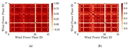
Figure 4.
Cross-correlation of both infeed and revenues for the portfolio of 46 (indexed 0 to 45) wind power plants. Clear similarities between correlation coefficients can be seen. Wind power plants 0 and 30 are significant outliers in terms of their cross-correlation. (a) Infeed correlation of wind power plants; (b) Revenue correlation for wind power plants.
4.2.1. Models
The results of the estimation of the marginal and copula models for the variance reduced portfolio are given in Table 6. As can be seen, both marginal models and copula estimation have significant similarities compared to the overall portfolio. The Student’s t copula is still best performing with regard to all defined GoF measures.
Table 6.
Fitted marginal model and copula for the variance reduced portfolio together with the quantile dependence plot of the best performing copula. The resemblance to the overall portfolio is uncanny.
4.2.2. Simulation and Optimized Hedging
Using the estimated marginal model for the portfolio infeed and the Student’s t copula the same variance minimization as with the total portfolio is performed. Result of the procedure are given in Table 7. The general findings are similar to the case with the total portfolio. Both hedging methods reduce variance and CVaR, with the volume hedge yielding a higher reduction in CVaR. Again, the variance minimizing hedge leads to a higher reduction in expected shortfall, i.e., a thinner adverse tail of the revenue distribution. Comparing the hedging volumes with the portfolio in Section 4 shows that smaller hedging volumes are decided upon in the optimal hedging positions (for both cases). In our study, we are resting the calculation of hedging volumes on fair prices of futures, i.e., expected spot prices. In reality there are examples of positive risk premiums for longer planning horizons [49], as typical for commodity markets. Reducing the necessity of using financial derivates for any hedging decision reduces the risk of experiencing adverse effects through the payment of risk premiums.
Table 7.
Risk assessment for the variance reduced portfolio with and without hedging. Both hedging methods reduce variance and CVaR significantly, with the minimal variance hedge outperforming the volume hedge with respect to expected shortfall. Optimal hedging volumes are reduced compared to the overall portfolio.
5. Discussion
The key contribution of this paper is the modeling the dependence structure of an actual wind portfolio infeed and German electricity prices with the help of copulas. To enable the estimation, models for cleaning the data of outliers, estimating deterministic seasonal components, and autoregressive models for the mean and variance components of the data are specified. With the standardized residuals of these marginal models, marginal distributions and a suitable copula model are estimated. Following the estimation of marginal models, distributions, and the dependence structure, price-infeed pairs could be simulated. On these values, a model was defined to estimate and optimize the risk arising from the modeled relationship of the variables. This could then be used to minimize the revenue variance by varying the quantity of different hedging products.
In an empirical example, all modeling steps were applied to infeed data from a large German virtual power plant operator and price data from the German market. A yearly seasonal model and an ARMA process was applied to the infeed data, with the residuals conforming to a Normal distribution. The price data was treated using an outlier model, a yearly and a weekly seasonal model and an ARMA-GARCH process.
We show that the revenue variance minimizing hedge using monthly futures contracts strongly reduces the Conditional Value-at-Risk and Expected Shortfall for a market actor facing joint price and volumetric risk. In this respect, the findings are similar to the study by [19] regarding the Danish market. Additionally, the hedge performs better than a simple volume hedge using the same instrument with regard to expected shortfall. Hence, we conclude that using the minimal revenue variance hedge with monthly futures can significantly reduce the price risk for a volatile electricity producer. Further, we show that a diversified portfolio with low cross-correlation in revenue streams from individual power plants improves risk aspects of the portfolio. Hedging volume can be reduced both with regard to a volume hedge and with regard to the minimum variance hedge. It can be therefore seen that value of an individual power plant does not only depend on the windiness of its location, but also its relationship to the remainder of the portfolio. This is especially true for risk averse decision-makers.
Some limitations remain. The risk model rests on strong assumptions, e.g., enforcing revenue neutrality, not all of which are realistic. Comparing the simulated distributions of both infeed and prices to the empirical ones, there remain differences for the price values. This suggests that there are further price drivers that are unaccounted for in the marginal model (see Appendix A). The empirical example limited itself to only one type of hedging instrument, primarily because illiquid markets preclude an application. Still, accounting for a broader set of derivates, e.g., weather derivates, would enhance the work. An interesting extension of our work is to include (stochastic) risk premiums together with an explicit modeling of the decision-makers risk aversion, in order to develop a decision support system for energy traders seeking to optimize their position.
Despite the limitations, we showed that volatile RES infeed and electricity prices show a complex relationship that is not fully captured by a simple Gaussian model only specifying correlation. Providing an initial method to manage risk subject to this relationship, we are motivating more research on complex risk management in electricity markets with high degree of RES penetration.
6. Materials and Methods
For the technical implementation of the estimation and simulation procedure, the Python programming language and associated statistical software packages are used in conjunction with packages for the R programming language.
Author Contributions
Investigation, J.K.; Supervision, W.K.; Visualization, J.K. and P.A.K.; Writing—original draft, P.A.K.; Writing—review & editing, J.K., P.A.K., and W.K. All authors have read and agreed to the published version of the manuscript.
Funding
This research received no external funding.
Acknowledgments
We would like to thank Next Kraftwerke for providing the data of their wind power portfolio.
Conflicts of Interest
The authors declare no conflict of interest.
Abbreviations
The following abbreviations are used in this manuscript:
| AIC | AKAIKE Information Criterion |
| ARMA | Autoregressive-Moving Average |
| BIC | Bayesian Information Criterion |
| CDF | Cumulative Distribution Function |
| CvM | Cramer-von-Mises |
| (C)VaR | (Conditional) Value-at-Risk |
| EPEX SPOT | European Power Exchange |
| ES | Expected Shortfall |
| GARCH | Generalized Autoregressive Conditional Heteroskedasticity |
| GoF | Goodness of Fit |
| iid | independent and identically distributed |
| KS | Kolmogorov-Smirnov |
| LTSC | Long-Term Seasonal Component |
| OTC | Over-the-counter |
| (P)ACF | (Partial) Autocorrelation Function |
| PCA | Principal Component Analysis |
| PPA(s) | Power Purchase Agreement(s) |
| RES | Renewable Energy Sources |
| STSC | Short-Term Seasonal Component |
Appendix A
Figure A1 shows that the standardized residuals simulated by the copula fit the data well. Their density is barely distinguishable from that defined by a kernel density estimation on the empirical standardized residuals. The deviation is larger when comparing the marginal models with the simulation. Obviously, there are aspects in price and infeed formation that are not accounted for by seasonality and ARMA-GARCH models.

Figure A1.
Comparison of the empirical and simulated distributions. (a) Comparison of standardized residuals of fitted marginal models and results of copula simulation. (b) Comparison of empirical distributions and re-transformed results of copula simulation.
Figure A1.
Comparison of the empirical and simulated distributions. (a) Comparison of standardized residuals of fitted marginal models and results of copula simulation. (b) Comparison of empirical distributions and re-transformed results of copula simulation.

References
- IEA. Germany 2020; IEA—International Energy Agency: Paris, France, 2020. [Google Scholar]
- Bundesministerium für Wirtschaft und Energie. Sechster Monitoring-Bericht zur Energiewende, Technical Report. 2018. Available online: https://www.bmwi.de/Redaktion/DE/Publikationen/Energie/sechster-monitoring-bericht-zur-energiewende.html (accessed on 9 July 2020).
- Bundeskartellamt. Monitoringbericht 2018, Technical Report. 2018. Available online: https://www.bundesnetzagentur.de/SharedDocs/Mediathek/Monitoringberichte/Monitoringbericht2018.pdf (accessed on 9 July 2020).
- Ketterer, J.C. The impact of wind power generation on the electricity price in Germany. Energy Econ. 2014, 44, 270–280. [Google Scholar] [CrossRef]
- Rintamäki, T.; Siddiqui, A.S.; Salo, A. Does renewable energy generation decrease the volatility of electricity prices? An analysis of Denmark and Germany. Energy Econ. 2017, 62, 270–282. [Google Scholar] [CrossRef]
- Mayer, K.; Trück, S. Electricity markets around the world. J. Commod. Mark. 2018, 9, 77–100. [Google Scholar] [CrossRef]
- Li, K.; Cursio, J.D.; Sun, Y. Principal component analysis of price fluctuation in the smart grid electricity market. Sustainability 2018, 10, 4019. [Google Scholar] [CrossRef]
- Bichler, M.; Gupta, A.; Ketter, W. Research commentary—Designing smart markets. Inf. Syst. Res. 2010, 21, 688–699. [Google Scholar] [CrossRef]
- Ketter, W.; Collins, J.; Reddy, P. Power TAC: A competitive economic simulation of the smart grid. Energy Econ. 2013, 39, 262–270. [Google Scholar] [CrossRef]
- Ketter, W.; Peters, M.; Collins, J.; Gupta, A. A multiagent competitive gaming platform to address societal challenges. Mis Q. 2016, 40, 447–460. [Google Scholar] [CrossRef]
- Ketter, W.; Peters, M.; Collins, J.; Gupta, A. Competitive benchmarking: an IS research approach to address wicked problems with big data and analytics. MIS Q. 2015. [Google Scholar] [CrossRef]
- Nicolosi, M.; Fürsch, M. The Impact of an increasing share of RES-E on the Conventional Power Market—The Example of Germany. Zeitschrift für Energiewirtschaft 2009, 33, 246–254. [Google Scholar] [CrossRef]
- Woo, C.; Horowitz, I.; Moore, J.; Pacheco, A. The impact of wind generation on the electricity spot-market price level and variance: The Texas experience. Energy Policy 2011, 39, 3939–3944. [Google Scholar] [CrossRef]
- Li, K.; Cursio, J.D.; Jiang, M.; Liang, X. The significance of calendar effects in the electricity market. Appl. Energy 2019, 235, 487–494. [Google Scholar] [CrossRef]
- Mbistrova, A.; Nghiem, A. The Value of Hedging New Approaches to Managing Wind Energy Resource Risk; Technical Report; WindEurope: Brussels, Belgium, 2017. [Google Scholar]
- McKinnon, R.I. Futures Markets, Buffer Stocks, and Income Stability for Primary Producers. J. Polit. Econ. 1967, 75, 844–861. [Google Scholar] [CrossRef]
- Oum, Y.; Oren, S.S. Optimal Static Hedging of Volumetric Risk in a Competitive Wholesale Electricity Market. Decis. Anal. 2010, 7, 107–122. [Google Scholar] [CrossRef]
- Oum, Y.; Oren, S.; Deng, S. Hedging quantity risks with standard power options in a competitive wholesale electricity market. Naval Res. Logist. 2006, 53, 697–712. [Google Scholar] [CrossRef]
- Pircalabu, A.; Jung, J. A mixed C-vine copula model for hedging price and volumetric risk in wind power trading. Quant. Financ. 2017, 17, 1583–1600. [Google Scholar] [CrossRef]
- Oum, Y.; Oren, S. VaR constrained hedging of fixed price load-following obligations in competitive electricity markets. Risk Decis. Anal. 2009, 1, 43–56. [Google Scholar] [CrossRef]
- Pircalabu, A.; Hvolby, T.; Jung, J.; Høg, E. Joint price and volumetric risk in wind power trading: A copula approach. Energy Econ. 2017, 62, 139–154. [Google Scholar] [CrossRef]
- Hain, M.; Schermeyer, H.; Uhrig-Homburg, M.; Fichtner, W. Managing renewable energy production risk. J. Bank. Financ. 2018, 97, 1–19. [Google Scholar] [CrossRef]
- Bartelj, L.; Gubina, A.F.; Paravan, D.; Golob, R. Risk management in the retail electricity market: The retailer’s perspective. In Proceedings of the IEEE PES General Meeting, PES 2010, Minneapolis, MN, USA, 25–29 July 2010. [Google Scholar]
- Patton, A.J. Copula Methods for Forecasting Multivariate Time Series. In Handbook of Economic Forecasting; Elsevier: Amsterdam, The Netherlands, 2013; Volume 2, pp. 899–960. [Google Scholar]
- Chen, X.; Han, J.; Zheng, T.; Zhang, P.; Duan, S.; Miao, S. A Vine-Copula Based Voltage State Assessment with Wind Power Integration. Energies 2019, 12, 2019. [Google Scholar] [CrossRef]
- Reboredo, J.C.; Ugolini, A.; Chen, Y. Interdependence Between Renewable-Energy and Low-Carbon Stock Prices. Energies 2019, 12, 4461. [Google Scholar] [CrossRef]
- Weron, R. Modeling and Forecasting Electricity Loads and Prices; John Wiley & Sons Ltd.: Oxford, UK, 2006; Volume 33. [Google Scholar]
- Meyer-Brandis, T.; Tankov, P. Multi-Factor Jump-Diffusion Models of Electricity Prices. Int. J. Theor. Appl. Financ. 2008, 11, 503–528. [Google Scholar] [CrossRef]
- Manner, H.; Alavi Fard, F.; Pourkhanali, A.; Tafakori, L. Forecasting the joint distribution of Australian electricity prices using dynamic vine copulae. Energy Econ. 2019, 78, 143–164. [Google Scholar] [CrossRef]
- Janczura, J.; Trück, S.; Weron, R.; Wolff, R.C. Identifying spikes and seasonal components in electricity spot price data: A guide to robust modeling. Energy Econ. 2013, 38, 96–110. [Google Scholar] [CrossRef]
- Ketter, W.; Collins, J.; Gini, M.; Gupta, A.; Schrater, P. Real-time tactical and strategic sales management for intelligent agents guided by economic regimes. Inf. Syst. Res. 2012, 23, 1263–1283. [Google Scholar] [CrossRef]
- Bollerslev, T. Generalized autoregressive conditional heteroskedasticity. J. Econ. 1986, 31, 307–327. [Google Scholar] [CrossRef]
- Ljung, G.M.; Box, G.E.P. On a measure of lack of fit in time series models. Biometrika 1978, 65, 297–303. [Google Scholar] [CrossRef]
- Sklar, A. Fonctions de répartition à n dimensions et leurs marges. Publ. l’Inst. Stat. L’Univ. Paris 1959, 8, 229–231. [Google Scholar]
- McNeil, A.J.; Frey, R.; Embrechts, P. Quantitative Risk Management: Concepts, Techniques and Tools; Princeton Series in Finance; Princeton University Press: Oxford, UK, 2005. [Google Scholar]
- Manner, H.; Reznikova, O. A survey on time-varying copulas: Specification, simulations, and application. Econ. Rev. 2012, 31, 654–687. [Google Scholar] [CrossRef]
- Embrechts, P.; Lindskog, F.; Mcneil, A. Modelling Dependence with Copulas and Applications to Risk Management. In Handbook of Heavy Tailed Distributions in Finance; Elsevier: Amsterdam, The Netherlands, 2003; pp. 329–384. [Google Scholar]
- Czado, C.; Schepsmeier, U.; Min, A. Maximum likelihood estimation of mixed C-vines with application to exchange rates. Stat. Model. Int. J. 2012, 12, 229–255. [Google Scholar] [CrossRef]
- Schmidt, T. Coping with Copulas. In Copulas: From Theory to Application in Finance; Rank, J., Ed.; Risk Books: London, UK, 2007. [Google Scholar]
- Patton, A.J. Modelling asymmetric Exchange Rate Dependence. Int. Econ. Rev. 2006, 47, 527–556. [Google Scholar] [CrossRef]
- Elberg, C.; Hagspiel, S. Spatial dependencies of wind power and interrelations with spot price dynamics. Eur. J. Oper. Res. 2015, 241, 260–272. [Google Scholar] [CrossRef]
- Coulon, M.; Powell, W.B.; Sircar, R. A model for hedging load and price risk in the Texas electricity market. Energy Econ. 2013, 40, 976–988. [Google Scholar] [CrossRef]
- Benth, F.E.; Kettler, P.C. Dynamic copula models for the spark spread. Quant. Financ. 2011, 11, 407–421. [Google Scholar] [CrossRef]
- Benth, F.E.; Meyer-Brandis, T. The information premium for non-storable commodities. J. Energy Mark. 2009, 2, 111–140. [Google Scholar] [CrossRef]
- Benth, F.E.; Jurate, S.B. Modeling and Pricing in Financial Markets for Weather Derivatives; World Scientific: Singapore, 2012; Volume 17. [Google Scholar]
- Burger, M.; Klar, B.; Müller, A.; Schindlmayr, G. A spot market model for pricing derivatives in electricity markets. Quant. Financ. 2004, 4, 109–122. [Google Scholar] [CrossRef]
- Kolos, S.P.; Ronn, E.I. Estimating the commodity market price of risk for energy prices. Energy Econ. 2008, 30, 621–641. [Google Scholar] [CrossRef]
- Näsäkkälä, E.; Keppo, J. Electricity load pattern hedging with static forward strategies. Manag. Financ. 2005, 31, 116–137. [Google Scholar] [CrossRef]
- Benth, F.E.; Sgarra, C. The risk premium and the Esscher transform in power markets. Stoch. Anal. Appl. 2012, 30, 20–43. [Google Scholar] [CrossRef][Green Version]


© 2020 by the authors. Licensee MDPI, Basel, Switzerland. This article is an open access article distributed under the terms and conditions of the Creative Commons Attribution (CC BY) license (http://creativecommons.org/licenses/by/4.0/).