Abstract
Recently, the development in combining point forecasts of electricity prices obtained with different length of calibration windows have provided an extremely efficient and simple tool for improving predictive accuracy. However, the proposed methods are strongly dependent on expert knowledge and may not be directly transferred from one to another model or market. Hence, we consider a novel extension and propose to use principal component analysis (PCA) to automate the procedure of averaging over a rich pool of predictions. We apply PCA to a panel of over 650 point forecasts obtained for different calibration windows length. The robustness of the approach is evaluated with three different forecasting tasks, i.e., forecasting day-ahead prices, forecasting intraday ID3 prices one day in advance, and finally very short term forecasting of ID3 prices (i.e., six hours before delivery). The empirical results are compared using the Mean Absolute Error measure and Giacomini and White test for conditional predictive ability (CPA). The results indicate that PCA averaging not only yields significantly more accurate forecasts than individual predictions but also outperforms other forecast averaging schemes.
1. Introduction
In recent years, we have observed a dynamic transformation of energy markets, which encompasses changes in the generation structure and the creation of new trading opportunities. Since the establishment of competitive power exchanges, a growing share of electricity has been traded in day-ahead markets, where offers are placed before the noon of the day preceding the delivery. To give traders the opportunity to balance deviations from positions contracted in the day-ahead market (due to the highly unpredictable generation from renewable sources), the spot markets have been complemented by intraday and balancing markets. Operation in such a complex environment becomes challenging for many market participants, as it requires taking various operational decisions, for example, generators need to decide, how much electricity to offer on a day-ahead market see [1] or how to structure the intraday trade [2]. Therefore, an accurate prediction of electricity prices becomes an important issue for utility managers.
The literature is rich in publications focusing on modelling and forecasting of spot prices (see [3,4] for a comprehensive review). At the same time, there are few articles, which are dedicated to intraday markets [2,5,6]. Most of them focus on a very short term—a few hours ahead—forecast, as in [7]. These types of models could not be directly used by utilities when making operational decisions. Hence, there is a need to develop and evaluate models, which will reflect the timeline of trading decisions, for example, the day-ahead forecast of intraday prices, as in [1]. On the other hand, electricity markets with their structural changes, seasonal fluctuations and occurrence of both positive and negative spikes, seek new forecasting methods, which will help to overcome some of these issues. As shown by the literature, forecast averaging may be particularly beneficial, when it is difficult to indicate a single, best preforming model—as in case of electricity prices.
The idea of averaging forecasts started about 50 years ago. Pioneering papers of [8,9] inspired many other authors to develop the area of combining forecasts. Since the late 60s, subject literature suggested that forecast combinations outperform individual models, see, e.g., [10,11,12]. Authors of [13] make a very important comment on forecast combination superiority. They claim that not only averaging different forecast performs better in terms of accuracy compared to any individual forecast, but also in practical usage, the combinations are always less risky. That is why in the subject literature a lot of averaging methods have been proposed and empirically compared. Surprisingly, the simple arithmetic mean (i.e., all individual forecasts are weighted equally) is for sure the most popular and incredibly reliable approach [14,15]. The same stands for taking the median of forecasts, which in some cases can even outperform a simple average. Using the ordinary least squares (OLS) method to utilize forecast combination is another easy to implement the approach in which weights are obtained from the linear regression, where individual forecasts are treated as the explanatory variables. Estimated weights, however, may exhibit unstable behavior (so-called bouncing betas) so we need to take into consideration that even slight fluctuations in the data can cause large changes in the final forecast. To prevent this [16] suggest using a constrained version of OLS, so-called CLS averaging, in which the weights are only positive and sum up to one.
The unwavering popularity of the simplest solutions is strong evidence of how difficult is the task of choosing the right tools to average the forecasts. Recently authors suggested that possibly, we should turn the question around and instead of wondering how to average individual forecasts, we should rather develop the tools to select, which forecasts are averaged in the first place. In [17] authors introduce a new approach based on a regularization technique. It allows not only to average but also to select a limited number of point forecasts. The authors propose new variants of the penalty function—egalitarian or partially egalitarian regularization. Even though the results were promising, the study was based only on a few dozen observations, and therefore definitely needs further research.
Moreover, recently [18,19] show that also the averaging of predictions obtained with the same model but calibrated to a different portion of data improves the predictive accuracy. In the recent papers [18,19,20] regarding averaging forecasts across calibration windows of different lengths, authors argue that combining forecasts from only a number of carefully selected calibration windows can significantly increase the forecasting performance and outperform the average of all predictions. Authors show that both for point [18,19] and probabilistic forecasts [20], considering the mix of short and long calibration windows brings statistically significant gains in terms of the forecasting accuracy. The intuition behind this result is that electricity prices exhibit both long- and short-term seasonality—therefore combining short and long calibration windows allow us to capture the specific data behaviour. On the other hand, the studies also show that an inappropriate choice of window lengths may noticeably lower the accuracy of the obtained predictions.
Although successful, the above methodology is based on a purely heuristic approach—in this paper, we propose an alternative automated (in the sense that it does not require any human decision) approach, based on the principal component analysis (PCA) method. The PCA was extensively investigated by [21,22,23] and has been successfully used for modelling big panels of data. In the approach, the information included in the panel is summarized with a few orthogonal factors. This allows to capture the correlation structure of the data set and to substantially reduce the dimensionality of the problem. The factors are next used to directly model the variables of interests [24,25,26] or to augment a small-scale econometric model [27,28,29]. In the energy literature, typical panels consist of electricity prices (or other fundamental variables) observed across different hours and locations [30,31,32]. The results indicate that a joint exploration of the whole panel leads to more accurate short- and mid-term forecasts.
The PCA approach could be also used to combine forecasts obtained from different models or/and model specifications. Although the literature recognizes the potential of PCA in forecast averaging [33,34], there are few articles where the method is successfully applied. In [14,33,35] static factors are employed to extract information from a panel of predictions coming from different models/experts, in order to obtain point forecast of the chosen macroeconomic variables. PCA was also adopted by [36], who used the method for the construction of prediction intervals of electricity spot prices. In all the above applications, factors are estimated with relatively small and diversified panels.
In this paper, an alternative setup is explored, in which the panel of predictions is homogeneous and consists of a large number of forecasts based on the same model estimated with different calibration windows, as in [18,19,20]. This setup gives new challenges. First, the panel of forecasts is not balanced because it consists of a relatively small number of predictions calculated with short calibration windows. Second, forecasts based on long windows are almost identical, as the growing sample size gives more stable parameter estimates. What is more, different days are characterized by different patterns of relationship between panel forecasts and actual prices. In order to solve some of the above problems, we normalize the predictions across the window size dimension. Next, we use both the time dependent moments of panel variables and factor estimates to calculate the price forecast. It is shown, that PCA combined with data standardization could be a promising alternative for other weighting schemes. Moreover, the method does not require an ad hoc selection of the calibration window length. In this research, the number of factors used for forecast averaging is either fixed and chosen ad-hoc or is dynamically selected with BIC information criteria. The results indicate that in case of slightly misspecified models, the proposed PCA–based procedure significantly outperforms both best performing ex–post selected calibration window and weighted averaged windows (WAW) approach [19]. In particular, the errors obtained with the model when forecasting the German day-ahead prices are almost 4% lower in terms of MAE in comparison to the optimal single calibration window and significantly better than any other considered averaging scheme. Finally, the aggregated outcomes show that PCA(1) using only one factor is the best among different PCA specifications. The averaging scheme utilizing information criteria to choose the number of factors is only slightly worse than PCA(1) and gives more robust results. Therefore, we recommend to use information criteria, such as BIC, for the automated selection of the number of factors.
The remainder of the paper is structured as follows. In Section 2, we present the datasets illustrating the German electricity market. Section 3 describes the experiment design, introduces variance stabilizing transformation (VST) and defines models used for forecasting of day-ahead and intraday prices. Next, in Section 4, we discuss forecast averaging schemes and introduce PCA forecast combination approach. The performance of the methods is evaluated in Section 5. Finally, the conclusions of the research are presented in Section 6.
2. Datasets
In order to test the proposed methodology, we utilize a number of datasets from the German market—each of them spans from 1 January 2015 to 15 August 2019. We consider two different price time series: the day-ahead hourly electricity prices (top panel in Figure 1) and the corresponding time series linked to the intraday market—the ID3 index hourly prices (bottom panel in Figure 1). According to the official rules by EPEX SPOT [37], the ID3 index is calculated as the volume-weighted average price of all trades within 3 h before the delivery of the product (up to 30 min before delivery). Apart from the price series, we use data for different types of exogenous variables: the day-ahead consumption prognosis (top panel in Figure 2) as well as the day-ahead wind and solar generation forecasts (respectively: middle and bottom panels in Figure 2). The wind generation forecast consists of aggregated forecasts of offshore and onshore generation forecasts.
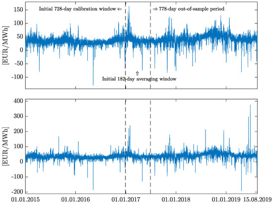
Figure 1.
Day-ahead (top) and intraday (ID3) (bottom) hourly electricity prices for German market, from 1 January 2015 to 15 August 2019. The first vertical dashed line marks the end of the 728-day calibration period and the second marks the end of the initial 182-day calibration window for averaging forecasts.
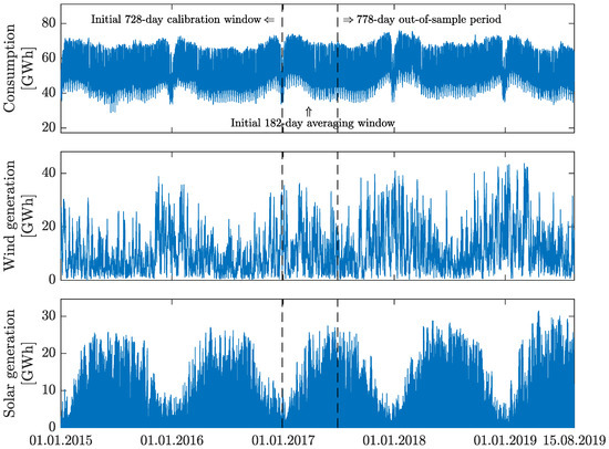
Figure 2.
Hourly consumption prognosis (top), wind (middle) and solar (bottom) hourly generation forecasts. Data span from 1 January 2015 to 15 August 2019. Note that for each series plot, the limits on the y axes are differ. The first vertical dashed line marks the end of the 728-day calibration period and the second marks the end of the initial 182-day calibration window for averaging forecasts.
In the recent paper [38], authors argue that wind and photovoltaic generation forecasting errors increase the system imbalance in Germany and these directly influence electricity prices. Hence, we additionally use two other fundamental factors that impact electricity prices: natural gas spot prices (top panel in Figure 3) and the spot price of European carbon emission allowances, more precisely, EUA—Emission Unit Allowance (see bottom panel in Figure 3). Note that, in contrast to electricity prices and generation forecasts, EUA and natural gas spot prices are quoted in a daily (not hourly) resolution. The missing (corresponding to the time change in March) or ‘doubled’ (corresponding to the reversion to standard time in October) values were replaced by the arithmetic mean of the neighbouring observations for the missing ones and the arithmetic mean of both values for ‘doubled’ hours.
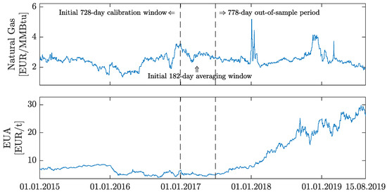
Figure 3.
Daily natural gas spot prices (top) and carbon emission allowances (EUA) spot prices (bottom). Data span from 1 January 2015 to 15 August 2019. Note that for each series plot, the limits on the y axes are differ. The first vertical dashed line marks the end of the 728-day calibration period and the second marks the end of the initial 182-day calibration window for averaging forecasts.
Descriptive statistics of the day-ahead and intraday price series are shown in Table 1. Although the mean of prices for both markets is very similar, the ID3 series exhibits greater variability and wider range of values. Day-ahead prices are negatively skewed (which is related with more frequent occurrence of bigger negative prices), the opposite can be observed for intraday prices. Finally, both electricity prices are leptokurtic, which confirms the occurrence of heavy tails caused by both positive and negative spikes. This feature has been widely discussed in the literature [3] and causes many difficulties while predicting future levels of electricity prices.

Table 1.
Descriptive statistics of the time series of the electricity prices in Germany in period from 1 January 2015 to 15 August 2019.
3. Methodology
3.1. Calibration Windows
Following the majority of forecasting literature, we consider a so-called rolling window scheme. Similarly to [18,19], instead of arbitrarily choosing a fixed calibration window length, we consider a set of 673 different window lengths—ranging from 56 (ca. two months) to 728 days (ca. two years)—obtained forecasts are later averaged (see Section 4). The first 728 (=) days are used for the initial model calibration. For each day in the period 29 December 2016 to 15 August 2019, we compute 24 point forecasts, one for each hour of the day. In addition, we use a 182-day fixed-length sample for the calibration of the averaging methods (see Section 4) to obtain the average forecast for each hour of the days between 29 June 2017 and 15 August 2019. The forecasts for all 778 days of the out-of-sample period are evaluated in Section 5. The end of the initial 728-day model calibration window (i.e., 1 January 2015 to 28 December 2016), as well as the end of the initial 182-day calibration window for averaging forecasts (i.e., 29 December 2016 to 29 June 2017) are indicated by dashed, vertical lines in Figure 1 and Figure 2.
3.2. Variance Stabilizing Transformation
Since electricity prices exhibit strong seasonality as well as spiky behaviour, we follow the recommendation of [39] and apply a so called variance stabilizing transformation (VST) to all datasets (to time series of prices as well as to exogenous variables). We apply the N-PIT transformation which is based on the so called probability integral transform. The transformed price for day d and hour h is given by:
where is the real observation for day d and hour h, is the empirical cumulative distribution function of in the calibration sample, and is an inverse of the normal distribution function. We calibrate the models to transformed time series and then apply inverse transformation to the computed forecasts in order to obtain the price predictions:
3.3. Models
In this study, we consider both day-ahead and intraday (ID3) prices from the German electricity market. The latter ones are usually forecasted during the delivery day and modeled with the use of a broader (more recent) pool of information, compared to day-ahead price forecasting. Most of the researchers [40,41,42] focus on very short forecasting horizons (from four to three hours before the delivery). Such a modeling setup, while allowing for higher accuracy of the predictions, do not leave enough time for utilizing the forecasts and adjusting trading strategies to market conditions. To tackle this issue, we decided to extend the forecasting horizon to 6 h, as it would enable market participants to exploit the future price movements and optimize the trades [43].
Intraday prices can also be predicted in a day-ahead manner, i.e., before submitting bids in the day-ahead market. This approach is particularly important when market participants need to decide, where to sell or buy energy (day ahead vs. intraday market). In such case, they need to predict day-ahead revenues from different trading strategies, as in [1]. Such approach can also be beneficial in terms of a decision-making process and risk management.
Let us focus first on the day-ahead spot prices, . In order to compute their point forecasts, autoregressive models with exogenous variables (ARX) estimated via the least-squares method are utilized. This type of models has been extensively used in the electricity price forecasting (EPF) literature [39,44,45]. The classical setup is expanded to include five exogenous variables: TSO forecasts of total load (), wind () and solar () generation, as well as spot prices of carbon emission allowances and natural gas. The final model, denoted by DA, is described by the following formula:
where , , are the lagged day-ahead prices from previous day, two days before and a week before. and refer to the minimum and the maximum price from day , is the last known price from the previous day. Finally, are weekday dummies accounting for the weekly seasonality. Note that the solar generation forecasts, , are included in the model only for hours 9–17, due to the obvious lack of generation during night and early morning hours.
The second task is to predict the day-ahead intraday price, namely the value of the ID3 index for the day d and hour h. We conduct the forecasting on the day preceding the delivery, as in the DA case. This implies that the intraday and spot prices are modelled in the same manner: all 24 prices for day d are forecasted at the same time, using the same pool of information. The model, denoted by IDA (Intraday Day-Ahead), has a structure similar to (3) and extends the model proposed by [1]. It assumes that the data generating process of intraday prices could be described by the following equation:
where , , are the lagged intraday prices. Due to the transaction timeline (see Figure 4) the prediction are performed at 10:00, when some of the intraday prices are yet not known. Therefore, a new variable, is constructed:
where is the volume-weighted average price of all transactions for a certain product, that have been made up to the moment of forecasting. In case there were no transactions, is replaced by the corresponding day-ahead price.
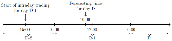
Figure 4.
Market trading timeline; the forecasting of and for day D is performed at 10:00 of day .
Finally, we build a model for a very short-term forecasting horizon for the intraday market (6 h before the delivery), which we denote by ID. It is based on the results presented in [40,46] and assumes that the ID3 price for day d and hour h is given by:
where refers to the ID3 price six hours before delivery and is the price for the hour h on the previous day. The is the volume-weighted average price of all transactions for a certain product, that has been made up to the 6 h before the delivery (the moment of forecasting). The next two variables link the intraday and day-ahead markets. refers to already known day-ahead price for the day d and hour h, while gives the newest information about price level difference between whose two markets. The rest of the predictors are just like in the DA and IDA models.
Note that for a better readability, we write to mark the product with the delivery i hours after (or before, for ) the product instead of using the correct notation .
4. Forecast Averaging
The literature shows that the accuracy of forecasts depends on the length of the calibration window used for the estimation of the model parameters. As shown in [18,19] this relationship could be non-monotonic and hence the selection of the optimal calibration window length becomes a complex task. On the other hand, the diversity of outcomes provides a strong motivation for using forecast averaging techniques, which could improve the forecasting performance of predictive models. Moreover, combining predictions could help to solve an issue of the optimal calibration window selection and reduce the model-specification risk.
Somehow interestingly, the concept of averaging forecasts across calibration windows of different lengths is relatively new in the field of electricity price forecasting. The recent articles [18,19] were the first papers tackling this overlooked problem in a systematic way.
4.1. Weighed Averaged Windows
The simple arithmetic average of the selected predictions is one of the most popular forecasts combining approaches. This method has been proved successful in a number of different studies across the econometric and forecasting literature. In the presented setup, the averaged window (AW) averaging scheme assumes equal weights for all forecasts estimated with the calibration windows of lengths .
Findings of [18,19] demonstrate that the reduction of the set of window lengths used for forecast averaging, , could improve the method performance. The authors indicate that the average of predictions obtained with three short and three long calibration windows, in most cases, outperforms the single ’optimal’ window as well as the average across all window lengths. The solution is also very efficient in terms of the computational cost—it requires calibrating the model to only six different sample lengths. [19] extended the idea of simple averaging and proposed an averaging scheme called weighed averaged windows (WAW). The weights are computed using the the inverse of the Mean Absolute Error (MAE) calculated over the averaging window of length (in [19])
where is the weight corresponding to a window of length on day d. is computed as an average of absolute forecast errors obtained from the model calibrated to a training sample of length over all hours of days :
where . Using this approach, the past performance of each window is taken into consideration and bigger weights are assigned to forecast obtained from windows that performed well in the past. Despite the computational efficiency and satisfying performance of this method, the choice of calibration window lengths has to be made in an ad-hoc manner and the inappropriate choice may have a significant impact on the forecasting performance.
4.2. BMA
Bayesian analysis offers an alternative approach to classical forecast assemble methods. As stated by [47], the weights based on bayesian model averaging (BMA) can be approximated by
where is the weight corresponding to the window of length and is a Bayesian Information Criterion. In should be noticed that since the models are estimated with different calibration windows, BIC is computed here over the forecast averaging window, not over the estimation sample. Then
where K is the number of parameters and defined similar to (10)
Since the penalty component in does not depend on the window length, , then the Equation (11) can be further simplified and becomes
It can be noticed that (14) is similar to the definition of WAW weights. The differences are two-fold: first, BMA weights are based on RMSE rather than MAE and second, they are raised to power , which represents the length of the forecast averaging window and shrinks weights of less accurate forecasts towards zero.
4.3. PCA Averaging
The majority of forecast combination approaches discussed in the literature, either use a small number of predictions or emphasise the need for prediction selection. Alternatively, one could utilize the information included in a big panel of forecasts by using the principal component analysis (PCA). The idea has been proposed by [14], who applied static factors to combine forecasts coming from different models. Similarly, [36] proposed the factor quantile regression averaging (FQRA) to construct prediction intervals using a panel of point forecasts. In both articles, PCA averaging is applied to relatively small and diversified panels of forecasts based on 27–66 individual models.
In the presented setup, the panel of forecast consists of 673 individual predictions acquired with different calibration windows. Since the growth of the window size, , leads to more stable parameter estimates, the forecasts obtained with long windows, for example, and are almost identical. This strong correlation, which is close to collinearity, impedes the classical, regression-based methods of forecast averaging. To avoid such problems, we propose a novel, fully-automated method for averaging forecasts, based on PCA.
In order to utilize all information from the averaging window, the data and predictions are treated as time series, with the time index, , representing consecutive hours. Similarly to the WAW approach, we use the information from previous days (in our setup ). Additionally, the data is extended by 24 forecasts of hourly prices from the day d. Therefore the final averaging window consists of observations. Let us denote by the prediction of the variable based on a calibration window of the length . The data set could be interpreted as a panel, with the first dimension representing time and the second dimension describing the size of a calibration window. The averaging algorithm consist of the following steps:
- For each time period t in the averaging window, estimate the mean () and standard deviation () of individual forecasts across different ;
- Standardize the predictions and the predicted variable;
- Estimate the first principal components, , of a panel , using the method described by [14,22]. Notice that the factors have a dimension as they include the information of the price forecasts on the day d. Based on the number of principal component K used in the model we denote the model by PCA(K);
- Run a regression using observations from the averaging window, without the last 24 observation;
- Compute the prediction of the normalized dependent variable on day d at hour h.and transform it into its original units
The role of standardization should be emphasised here. The mean, which changes between days, could be interpreted as the first common factor affecting the panel of forecasts. In particular, it represents the forecast based on long calibration windows. The predictions for big are, by construction, very similar to each other and have the largest input to the mean. On the other hand, the impact of long windows on the demeaned panel is balanced by larger (in absolute terms) and more variable deviations from mean for short calibration windows.
The standard deviation represents the forecast uncertainty and increases when short and long windows give different predictions. If the original data was used to estimate the principal components, the days with the highest risk would have the largest input to the panel variance and hence would impact strongly factor estimates. Thanks to standardization, all days are equally represented by common factors and the outcomes are stable, even when the outliers are included in the sample used for forecast averaging. On the other hand, in the future work one can try to use the information about standard deviation and include the variance to the model for probabilistic forecasting, for example to construct the prediction intervals with quantile regression or its generalizations [48,49].
It should be noticed here that the described algorithm is conditioned on several factors, K, used in the regression (17). To make the choice of K data-driven, we use Bayesian information criteria (BIC):
where is an estimated residuals variance from the model (17) with K components. For each day d, the optimal is chosen, which minimizes the corresponding .
5. Results
5.1. Forecast Evaluation
We use the Mean Absolute Error (MAE) for the full out-of-sample test period of days (i.e., 26.06.2017 to 15.08.2018, see Figure 1) as the main evaluation criterion. In the paper, two measures are considered
where is the prediction error at day d and hour h based on the averaging method i or for models without averaging. The first measure, describes the forecast accuracy for a given day, d, and is later use for statistical comparison of individual approaches. Finally describes the overall performance of the method . Recall, that the MAE is the most commonly used measure for evaluation forecast accuracy. In the case of electricity markets, it reflects the average deviation of the revenue from selling 1 MWh from its expected level.
Given a number of results, it is hard to properly rank the models accuracy. To solve this issue, following [39,44], we introduce the mean percentage deviation from the best (m.p.d.f.b.) benchmark, inspired by the m.d.f.b. measure used in [50,51] for comparing models. The m.p.d.f.b. measure for model i compares the model’s performance to the best benchmark (it is the best performing calibration window length for each of models :
The obtained MAE values can be used to provide a ranking of models. Unfortunately, they do not allow to draw statistically significant conclusions on the outperformance of the forecasts of one model by those of another. Therefore, the conditional predictive ability (CPA) test of Giacomini and White [52] is used to compare competitive outcomes. Note that the CPA test could be viewed as a generalization of the popular Diebold and Mariano [53] test for unconditional predictive ability. Here, the test statistic is computed using the vector of average daily :
where is the mean absolute error of forecast obtained with model i on day d. For each pair of window sets and each model we compute the p-value of the CPA test with null in the regression [52]:
where contains elements from the information set on day , i.e., a constant and .
5.2. Point Forecast Results
As mentioned earlier, in this paper we consider training samples of lengths ranging from 56 to 728 days. Since the same model calibrated to a sample of different lengths produces differing forecasts, this gives us 673 different ‘sub-models’ for each of the models. The forecasting performance is evaluated separately for each calibration window, and the results are shown in Figure 5—each dot represents the MAE of forecasts obtained by calibrating the model to a sample of a certain length. Interestingly, the curves for and models are not monotonic as one may expect, the forecasting error does not strictly fall with the increase of the calibration sample length. This behavior of MAE may suggest that the models are slightly misspecified due to, for example, assumed linearity, time-invariant parameters or omitted variables. In such a case, the parameter estimates are inconsistent and do not converge to their true values. On the other hand, the curve for the model is descending. The forecasting accuracy of this model increases with the length of the calibration window, leaving little room for an improvement for averaging techniques.
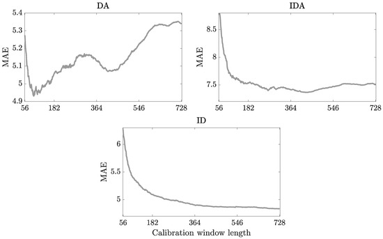
Figure 5.
Mean absolute error as the function of the calibration sample length. The results for (top-left), (top-right) and (bottom) models are evaluated over the whole 778-day out-of-sample test period.
Another conclusion that can be drawn is that none of the calibration window lengths would be the ‘optimal’ choice for all models—the best-performing calibration window for model is 95 days, whereas for the best forecasting performance would be achieved when calibrating the model on a 438-day sample and for the longest calibration samples perform the best. This diversified pattern of behavior shows that there is a need for the more robust way of selecting the length of calibration windows.
5.3. Averaging Results
Table 2 presents MAE and m.p.d.f.b results for forecasts obtained with the shortest (56-days), the one-year long (364-days) and the longest (728-days) calibration windows and compare them against a benchmark: the best (optimal) (ex–post) calibration window length. Next, outcomes of different averaging technique are reported, starting with AW/WAW and BMA for all , AW/WAW and BMA for six selected window sizes as in [18,19,20] and PCA averaging with 1 to 4 factors. Finally, outcomes of PCA(BIC) scheme are presented, in which the number of components is estimated using BIC information criterion. The results are displayed in absolute terms (MAE) and relative to the benchmark (computed as a percentage difference, %chng).
Table 2.
Mean absolute errors (MAE) and mean percentage deviation from the best benchmark (m.p.d.f.b) of the forecast obtained with all three considered models in the 778-days out-of-sample period from 26 June 2017 to 15 August 2019. In the first four rows reported result for models calibrated on single in-sample length, whereas the bottom rows correspond to models using one of the averaging techniques. The percentage change compared to the best ex–post length of calibration window is reported in columns %chng. Note that the best model in terms of MAE is underlined.
The presented measures are computed with data ranging from 26 June 2017 to 15 August 2019, it is a 778-days long out-of-sample period. The three considered models, it is , and , are evaluated separately and their outcomes are shown in consecutive columns. Finally, the average performance of analyzed forecasting schemes is described by m.p.d.f.b. The results lead to several important conclusions:
- In case of and models, the averaged forecasts are more accurate than any of the individual predictions, including those based on the best ex–post calibration window length. The gains reach up to 3.841% and 2.097% for and , respectively. At the same time, none of the combined predictions provide results better than the benchmark for model. This confirms our expectation that averaging across different calibration window lengths may not lead to any improvement of forecast accuracy in case of well-specified models, which parameters can be consistently estimated.
- When two similar averaging schemes, AW and WAW, are compared, the results indicate that the extension of WAW, originally proposed by [19], outperforms the simple arithmetic mean. The superiority of WAW is obtained for all models and both ranges of window lengths, .
- The outcomes for the AW/WAW averaging scheme show that the pre-selection of six window lengths improves the forecast accuracy only in case of misspecified models: and . At the same time, results for suggest that, for well-specified models, the ad hoc reduction of the dimension increases substantially the MAE measure.
- Results for the BMA scheme perform much worse in terms of MAE for the and models compared to non-Bayesian approaches. The situation changes for model, when BMA is the most accurate among forecast averaging schemes but still worse than the best individual model.
- The PCA forecast averaging approaches lead to more accurate predictions of and than any other combining schemes. They reduce MAE, relatively to the benchmark, by 3.841% and 2.097%, respectively. For model, all averaging schemes perform worse than the 2-year calibration window. Still, PCA is exhibits the smallest forecast error among presented methods.
- The PCA based methods perform similarly, regardless of the number of factors used for forecast averaging. One could observe small differences between markets that indicate that PCA(4) is on average the most efficient.
- BIC information criterion is shown to be helpful in selecting the number of components. Although it could not beat the best PCA specification for individual models (, and ), it works very well on average.
Note that in the presented setup, forecast averaging weights are estimated using predictions of previous days. Although it is out of scope of this paper, we conducted a limited study to analyze, how the reduction of to 60 days affects the results. It turned out that the choice of has a minor impact on outcomes and does not alter the major conclusions. It seems that the relative accuracy of PCA increases for longer forecast averaging windows, as more information improves estimation of principle components.
Finally, the results are evaluated with the Giacomini-White test [52] for the norm of order one. The outcomes are presented in Figure 6, on which a non-black square indicates that the forecasts of a model on the X-axis are statistically more accurate than the forecasts of a model on the Y-axis. The results confirm previous findings and show that PCA schemes outperform other methods, when the day-ahead forecasts are considered. This outcome is supported by two observations:
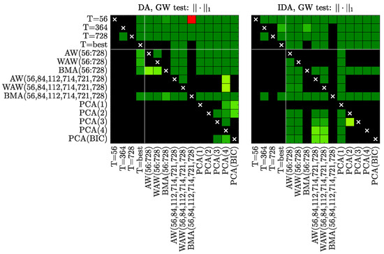
Figure 6.
Results of the conditional predictive ability (CPA) test [52] for forecasts of all considered models. We use a heat map to indicate the range of the p-values—the closer they are to zero (→ dark green) the more significant is the difference between the forecasts of a model on the X-axis (better) and the forecasts of a model on the Y-axis (worse).
- PCA(4) and PCA(1) are significantly the most accurate for and models, respectively.
- PCA(1) is not statistically worse than any of the predictions apart from some other PCA specifications.
When the model is considered, the outcomes show that approaches based on the longest and the best calibration window lengths provide forecasts of the same accuracy, which outperform almost all other prediction methods. Moreover, for this market,
- Forecasts obtained with PCA(3) and BMA(56,84,112,714,721,728) are the only predictions, which are not statistically worse than results for or .
- BMA(56,84,112,714,721,728) forecasts are statistically better than those obtained with all other averaging schemes apart from PCA(3).
Finally, it could be noticed that PCA(BIC) is rarely outperformed by other PCA specifications. This result confirms that BIC is useful in determining the optimal number of components used for averaging and hence could be an attractive alternative to the ad hoc choice of K.
6. Conclusions
In this paper, we model and predict hourly electricity prices on the German market. We consider three forecasting setups: a day-ahead forecast of spot prices, a day-ahead forecast of intraday prices and a short-term, 6 h ahead prediction of index. The analyzed problems reflect the decision process of market participants and could help in optimizing the selling/buying strategy as in [1,2].
We propose a novel approach for calculating the predictions of electricity prices, which utilize forecasts based on models calibrated to windows of different lengths. We extend the idea introduced in [18,19], which focuses on an ad hoc selection of the best set of calibration windows. In this study, we propose a principal component analysis (PCA) method for forecast averaging, which enables the automatic aggregation of information included in the large panel of predictions. The results indicate that the PCA averaging scheme can, on average, reduce the MAE measure of forecast accuracy, relative to the best ex–post calibration window length. It also outperforms other forecast averaging approaches, such as AW, WAW and BMA.
Furthermore, we show that , and models have different characteristics, which correlate with the forecast horizon. The performance of day-ahead forecasts of spot and intraday prices does not improve with the growth of the calibration window length, whereas the short-term predictions of ID3 get more accurate for the longest estimation windows. This difference impacts the potential gains from forecast averaging. For the model, none of the proposed methods could outperform the forecasts based on the longest calibration window. At the same time, the averaging—and in particular PCA forecast combination—results in a significant decrease of MAE for and models. The forecast accuracy improves relative to the benchmark, by almost 4% for PCA(4) scheme and model. In the case of model, the error reduction reaches 2% for PCA(1) approach.
Finally, the results indicate that the two PCA forecast averaging methods, with one or four components, provide the most accurate predictions. PCA(1) is statistically not worse than any of the AW or WAW forecast combination schemes and outperforms all approaches for IDA. At the same time, PC(4) has on average the lowest MAE, measured by m.p.d.f.b (mean percentage deviation from the best). The PCA method, with the number of components selected with BIC information criterion, provides forecasts which are only slightly worse than those obtained with PCA(4) and PCA(1). Hence, it could be viewed as an interesting alternative for ad hoc selection of the number of components. We believe that these results encourage further research on PCA forecast averaging, which could be extended to interval and probabilistic forecasting and be applied to other commodity markets.
Author Contributions
Conceptualization, K.M.; Investigation, K.M., T.S. and B.U.; Software, B.U. and K.M.; Validation, K.M.; Writing—original draft, T.S.; Writing—review & editing, K.M. and B.U. All authors have read and agreed to the published version of the manuscript.
Funding
This work was partially supported by the Ministry of Science and Higher Education (MNiSW, Poland) through Diamond Grant No. 0199/DIA/2019/48 (to B.U.) and German Research Foundation (DFG, Germany) and the National Science Center (NCN, Poland) through BEETHOVEN grant no. 2016/23/G/HS4/01005 (to T.S.) and SONATA grant no. 2016/21/D/HS4/00515 (to K.M.).
Conflicts of Interest
The authors declare no conflict of interest.
References
- Maciejowska, K.; Nitka, W.; Weron, T. Day-ahead vs. Intraday—Forecasting the price spread to maximize economic benefits. Energies 2019, 12, 631. [Google Scholar] [CrossRef]
- Kath, C.; Ziel, F. The value of forecasts: Quantifying the economic gains of accurate quarter-hourly electricity price forecasts. Energy Econ. 2018, 76, 411–423. [Google Scholar] [CrossRef]
- Weron, R. Electricity price forecasting: A review of the state-of-the-art with a look into the future. Int. J. Forecast. 2014, 30, 1030–1081. [Google Scholar] [CrossRef]
- Nowotarski, J.; Weron, R. Recent advances in electricity price forecasting: A review of probabilistic forecasting. Renew. Sustain. Energy Rev. 2018, 81, 1548–1568. [Google Scholar] [CrossRef]
- Kiesel, R.; Paraschiv, F. Econometric analysis of 15-minute intraday electricity prices. Energy Econ. 2017, 64, 77–90. [Google Scholar] [CrossRef]
- Monteiro, C.; Ramirez-Rosado, I.; Fernandez-Jimenez, L.; Conde, P. Short-term price forecasting models based on artificial neural networks for intraday sessions in the Iberian electricity market. Energies 2016, 9, 721. [Google Scholar] [CrossRef]
- Uniejewski, B.; Marcjasz, G.; Weron, R. On the importance of the long-term seasonal component in day-ahead electricity price forecasting: Part II—Probabilistic forecasting. Energy Econ. 2019, 79, 171–182. [Google Scholar] [CrossRef]
- Bates, J.M.; Granger, C.W.J. The Combination of Forecasts. Oper. Res. Q. 1969, 20, 451–468. [Google Scholar] [CrossRef]
- Crane, D.; Crotty, J. A two-stage forecasting model: Exponential smoothing and multiple regression. Manag. Sci. 1967, 13, B501–B507. [Google Scholar] [CrossRef]
- Timmermann, A.G. Forecast combinations. In Handbook of Economic Forecasting; Elliott, G., Granger, C.W., Timmermann, A., Eds.; Elsevier: Amsterdam, The Netherlands, 2006; pp. 135–196. [Google Scholar]
- Wallis, K.F. Combining forecasts—Forty years later. Appl. Financ. Econ. 2011, 21, 33–41. [Google Scholar] [CrossRef]
- Nowotarski, J.; Weron, R. To combine or not to combine? Recent trends in electricity price forecasting. ARGO 2016, 9, 7–14. [Google Scholar]
- Hibon, M.; Evgeniou, T. To combine or not to combine: Selecting among forecasts and their combinations. Int. J. Forecast. 2005, 21, 15–24. [Google Scholar] [CrossRef]
- Stock, J.H.; Watson, M.W. Combination forecasts of output growth in a seven-country data set. J. Forecast. 2004, 23, 405–430. [Google Scholar] [CrossRef]
- Genre, V.; Kenny, G.; Meyler, A.; Timmermann, A. Combining expert forecasts: Can anything beat the simple average? Int. J. Forecast. 2004, 29, 108–121. [Google Scholar] [CrossRef]
- Raviv, E.; Bouwman, K.E.; van Dijk, D. Forecasting day-ahead electricity prices: Utilizing hourly prices. Energy Econ. 2015, 50, 227–239. [Google Scholar] [CrossRef]
- Diebold, F.X.; Shin, M. Machine learning for regularized survey forecast combination: Partially-egalitarian LASSO and its derivatives. Int. J. Forecast. 2019, 35, 1679–1691. [Google Scholar] [CrossRef]
- Hubicka, K.; Marcjasz, G.; Weron, R. A note on averaging day-ahead electricity price forecasts across calibration windows. IEEE Trans. Sustain. Energy 2019, 10, 321–323. [Google Scholar] [CrossRef]
- Marcjasz, G.; Serafin, T.; Weron, R. Selection of Calibration Windows for Day-Ahead Electricity Price Forecasting. Energies 2018, 11, 2364. [Google Scholar] [CrossRef]
- Serafin, T.; Uniejewski, B.; Weron, R. Averaging predictive distributions across calibration windows for day-ahead electricity price forecasting. Energies 2019, 12, 2561. [Google Scholar] [CrossRef]
- Stock, J.H.; Watson, M.W. Forecasting Using Principal Components from a Large Number of Predictors. J. Am. Stat. Assoc. 2002, 97, 1167–1179. [Google Scholar] [CrossRef]
- Bai, J.; Ng, S. Determining the Number of Factors in Approximate Factor Models. Econometrica 2002, 70, 191–221. [Google Scholar] [CrossRef]
- Bai, J. Inferential theory for factor models of large dimensions. Econometrica 2003, 71, 135–171. [Google Scholar] [CrossRef]
- Boivin, J.; Ng, S. Understanding and Comparing Factor-Based Forecasts. Int. J. Cent. Bank. 2005, 1. [Google Scholar] [CrossRef]
- Eickmeier, S.; Ziegler, C. How successful are dynamic factor models at forecasting output and inflation? A meta-analytic approach. J. Forecast. 2008, 27, 237–265. [Google Scholar] [CrossRef]
- Stock, J.H.; Watson, M.W. Generalized Shrinkage Methods for Forecasting Using Many Predictors. J. Bus. Econ. Stat. 2012, 30, 481–493. [Google Scholar] [CrossRef]
- Bernanke, B.; Boivin, J.; Eliasz, P. Measuring the Effects of Monetary Policy: A Factor-Augmented Vector Autoregressive (FAVAR) Approach. Q. J. Econ. 2005, 120, 387–422. [Google Scholar]
- Koop, G.; Korobilis, D. UK macroeconomic forecasting with many predictors: Which models forecast best and when do they do so? Econ. Model. 2011, 28, 2307–2318. [Google Scholar] [CrossRef]
- Banerjee, A.; Marcellino, M.; Masten, I. Forecasting with factor-augmented error correction models. Int. J. Forecast. 2014, 30, 589–612. [Google Scholar] [CrossRef]
- Garcia-Martos, C.; Rodriguez, J.; Sanchez, M. Forecasting electricity prices by extracting dynamic common factors: Application to the Iberian Market. IET Gener. Transm. Distrib. 2012, 6, 11–20. [Google Scholar] [CrossRef]
- Garcia-Martos, C.; Rodriguez, J.; Sanchez, M. Electricity Prices Forecasting by Averaging Dynamic Factor Models. Energies 2016, 9, 600. [Google Scholar]
- Maciejowska, K.; Weron, R. Forecasting of daily electricity prices with factor models: Utilizing intra-day and inter-zone relationships. Comput. Stat. 2015, 30, 805–819. [Google Scholar] [CrossRef]
- Huang, H.; Lee, T.H. To Combine Forecasts or to Combine Information? Econom. Rev. 2010, 29, 534–570. [Google Scholar] [CrossRef]
- Chan, Y.L.; Stock, J.H.; Watson, M.W. A dynamic factor model framework for forecast combination. Int. J. Forecast. 1999, 22, 283–300. [Google Scholar] [CrossRef]
- Poncela, P.; Rodriguez, J.; Sanchez-Mangas, R.; Senra, E. Forecast combination through dimension reduction techniques. Int. J. Forecast. 2011, 27, 224–237. [Google Scholar] [CrossRef]
- Maciejowska, K.; Nowotarski, J.; Weron, R. Probabilistic forecasting of electricity spot prices using Factor Quantile Regression Averaging. Int. J. Forecast. 2016, 32, 957–965. [Google Scholar] [CrossRef]
- EPEXSpot. Description of Epex Spot Market Indices; European Power Exchange: Paris, France, 2020; Available online: https://www.epexspot.com/en/indices (accessed on 2 March 2020).
- Goodarzi, S.; Perera, H.; Bunn, D. The impact of renewable energy forecast errors on imbalance volumes and electricity spot prices. Energy Policy 2019, 134, 110827. [Google Scholar] [CrossRef]
- Uniejewski, B.; Weron, R.; Ziel, F. Variance Stabilizing Transformations for Electricity Spot Price Forecasting. IEEE Trans. Power Syst. 2018, 33, 2219–2229. [Google Scholar] [CrossRef]
- Uniejewski, B.; Marcjasz, G.; Weron, R. Understanding intraday electricity markets: Variable selection and very short-term price forecasting using LASSO. Int. J. Forecast. 2019, 35, 1533–1547. [Google Scholar] [CrossRef]
- Narajewski, M.; Ziel, F. Econometric modelling and forecasting of intraday electricity prices. J. Commod. Mark. 2019. [Google Scholar] [CrossRef]
- Janke, T.; Steinke, F. Forecasting the price distribution of continuous intraday electricity trading. Energies 2019, 12, 4262. [Google Scholar] [CrossRef]
- Edoli, E.; Fiorenzani, S.; Vargiolu, T. Optimal Trading Strategies in Intraday Power Markets. In Optimization Methods for Gas and Power Markets: Theory and Cases; Palgrave Macmillan: London, UK, 2016; pp. 161–184. [Google Scholar]
- Ziel, F.; Weron, R. Day-ahead electricity price forecasting with high-dimensional structures: Univariate vs. multivariate modeling frameworks. Energy Econ. 2018, 70, 396–420. [Google Scholar] [CrossRef]
- Uniejewski, B.; Weron, R. Efficient forecasting of electricity spot prices with expert and LASSO models. Energies 2018, 11, 2039. [Google Scholar] [CrossRef]
- Marcjasz, G.; Uniejewski, B.; Weron, R. Beating the Naïve—Combining LASSO with Naïve Intraday Electricity Price Forecasts. Energies 2020, 13, 1667. [Google Scholar] [CrossRef]
- Hansen, B.E. Least-squares forecast averaging. J. Econom. 2008, 146, 342–350. [Google Scholar] [CrossRef]
- Koenker, R.W. Quantile Regression; Cambridge University Press: Cambridge, UK, 2005. [Google Scholar]
- Uniejewski, B.; Weron, R. Regularized Quantile Regression Averaging for probabilistic electricity price forecasting. Energy Econ. 2020, submitted. [Google Scholar]
- Weron, R.; Misiorek, A. Forecasting spot electricity prices: A comparison of parametric and semiparametric time series models. Int. J. Forecast. 2008, 24, 744–763. [Google Scholar] [CrossRef]
- Nowotarski, J.; Raviv, E.; Trück, S.; Weron, R. An empirical comparison of alternate schemes for combining electricity spot price forecasts. Energy Econ. 2014, 46, 395–412. [Google Scholar] [CrossRef]
- Giacomini, R.; White, H. Tests of conditional predictive ability. Econometrica 2006, 74, 1545–1578. [Google Scholar] [CrossRef]
- Diebold, F.X.; Mariano, R.S. Comparing predictive accuracy. J. Bus. Econ. Stat. 1995, 13, 253–263. [Google Scholar]
© 2020 by the authors. Licensee MDPI, Basel, Switzerland. This article is an open access article distributed under the terms and conditions of the Creative Commons Attribution (CC BY) license (http://creativecommons.org/licenses/by/4.0/).