Analysis of Relaxation Time of Temperature in Thermal Response Test for Design of Borehole Size
by
 , , and
Hobyung Chae
1, 
Katsunori Nagano
1,*, 
Yoshitaka Sakata
1,
Takao Katsura
1,
Ahmed A. Serageldin
1,2 and
Takeshi Kondo
3 1
Graduate School of Engineering, Hokkaido University, N13-W8, Sapporo 060-8628, Japan
2
Mechanical Power Engineering Department, Faculty of Engineering at Shoubra, Benha University, Shoubra 11629, Egypt
3
NIKKEN SEKKEI Research Institute, 3-737, Kanda Ogawamachi, Chiyoda-ku, Tokyo 101-0052, Japan
*
Author to whom correspondence should be addressed.
Energies 2020, 13(13), 3297; https://doi.org/10.3390/en13133297
Submission received: 4 May 2020
/
Revised: 18 June 2020
/
Accepted: 18 June 2020
/
Published: 27 June 2020
(This article belongs to the Special Issue Thermal Response Tests for Shallow Geothermal Systems)
Abstract
:A new practical method for thermal response test (TRT) is proposed herein to estimate the groundwater velocity and effective thermal conductivity of geological zones. The relaxation time of temperature (RTT) is applied to determine the depths of the zones. The RTT is the moment when the temperature in the borehole recovers to a certain level compared with that when the heating is stopped. The heat exchange rates of the zones are calculated from the vertical temperature profile measured by the optical-fiber distributed temperature sensors located in the supply and return sides of a U-tube. Finally, the temperature increments at the end time of the TRT are calculated according to the groundwater velocities and the effective thermal conductivity using the moving line source theory applied to the calculated heat exchange rates. These results are compared with the average temperature increment data measured from each zone, and the best-fitting value yields the groundwater velocities for each zone. Results show that the groundwater velocities for each zone are 2750, 58, and 0 m/y, whereas the effective thermal conductivities are 2.4, 2.4, and 2.1 W/(m∙K), respectively. The proposed methodology is evaluated by comparing it with the realistic long-term operation data of a ground source heat pump (GSHP) system in Kazuno City, Japan. The temperature error between the calculated results and measured data is 6.4% for two years. Therefore, the proposed methodology is effective for estimating the long-term performance analysis of GSHP systems.
1. Introduction
Ground source heat pump (GSHP) systems utilizing the ground as a heat source or heat sink have been recognized as being high performance and environmentally friendly [1,2,3]. The studies on the GSHP system with various types of heat exchanger have studied how to supply heating and cooling to houses and the buildings [4,5]. Among them, borehole heat exchangers (BHEs), composed of vertical closed-loops, are preferred because of their high efficiency and minimal installation space requirement in expensive neighborhoods [6]. The reason for the high efficiency of the vertical loop type is that they can use the stable heat source from the relatively deeper ground, compared with the horizontal loop type which uses the heat source of the ground surface affected by the weather condition. The design of BHEs primarily depends on the thermal properties of soil as the design parameter. The main parameters are the effective thermal conductivity of the soil and the borehole thermal resistance obtained from the analysis of a thermal response test (TRT). The conventional TRT analysis method proposed by Mogensen [7] involves the analysis of the average temperature of a circulating fluid measured in an inlet and outlet of a U-tube using an infinite line source model based on least-squares approximation [8]. Its simple process resulted in its frequent use. Considering only conduction heat transfer, this method causes no significant problems when the groundwater is less than 0.1 m/d [9]. Fossa et al. [10] conducted a pulsated TRT where the heat rate at the heat carrier fluid is deliberately varied according to a series of on/off heat pulses able to resemble real GCHP operating conditions. The effective thermal conductivity of the soil and the borehole thermal resistance were estimated using the infinite line source model, the finite line source model and the resistance/capacitance approach, and its results were compared. However, rapid groundwater flows render the effective thermal conductivity artificially high. This high value might result in over/underdesigned BHEs. Accordingly, BHEs must be designed to reflect not only the thermal properties of the soil, but also the groundwater velocities in areas with rapid groundwater flows.
Groundwater flow can improve the heat transfer efficiency of the ground, and hence, provide better performance of the GSHP system. Researchers have studied the effect of groundwater flow on the performances of GSHP systems [11,12,13,14,15]. However, BHEs have not been designed to reflect the on-site groundwater velocity, which is difficult to estimate when the groundwater flow is moderate or slow. Wanger et al. [16] reported that the analytical approach in advection-influenced conditions can be considered when the Darcy velocity exceeds 0.1 m/d for TRT analysis. Another factor is the TRT period. The TRT is generally operated within a limited time owing to the required construction time and cost. Hence, researchers [9,17,18,19,20,21] determined the minimum TRT durations that are sufficient to estimate the thermal properties. However, the operating time of the TRT must be sufficiently long to observe the effects of moderate or slow groundwater flows. This is clearly shown in the temperature change according to the Darcy velocity [19]. Groundwater flow speeds can affect the time when the soil temperature converges during the TRT. If the time mentioned above is long, then the groundwater velocity can be regarded as low. In other words, it is time-consuming to observe the effects of slow groundwater flows by temperature changes. The suggested TRT periods [9,17,18,19,20,21] are insufficient to estimate moderate or slow groundwater flows through TRT analysis.
Wagner et al. [22] conducted both a tank experiment and a field experiment for the TRT to determine the hydraulic conductivity in an aquifer. They set the hydraulic conductivity ranges according to the soil properties, such as grain size, thermal conductivity, and porosity. Each value of these properties was utilized to calculate the temperature of the circulating fluid based on moving line source (MLS) theory. The calculated temperature results were then compared with the TRT data. The optimal fitting result yielded the hydraulic conductivity of the soil. Although appropriate results were demonstrated, their approach required not only a sufficient preliminary investigation for the thermal parameters of the soils, but also tens of thousands of iterative calculations. In our previous study [23], a practical approach was proposed for the simultaneous determination of both the groundwater velocity and the effective thermal conductivity of soils. Furthermore, the relationship between the groundwater velocity and effective thermal conductivity was obtained. The effective thermal conductivity and groundwater velocity were estimated to be 4.7 and 120 m/y, respectively. The estimated effective thermal conductivity was much higher than that of the soil in the test site, where the ground was primarily composed of sandy gravel, even though the calculated temperature matched well with the TRT data. The high value is attributable to the ground being considered as a homogeneous medium in the methodology. Furthermore, if the TRT is performed for a long term, the temperature difference between the calculated temperature and the TRT data will increase; the calculated temperature reflecting the groundwater flow will converge, whereas the measured data will increase gradually. Therefore, the thermal properties including the groundwater flow speeds in multiple layers must be estimated in the TRT analysis method.
The methods to determine the thermal properties in a multilayer using the optical fiber distributed temperature sensing (DTS) technique have been proposed [24,25,26,27,28,29,30]. Fujii et al. [27] utilized optical fiber DTS to measure the temperature–time profile of circulating fluids in U-tubes during a TRT. The measured profiles were history matched with the cylindrical source function [8]. McDaniel et al. [30] provided a detailed description of variability in the subsurface heat transfer using the optical fiber DTS with laboratory thermophysical measurements. Sakata et al. [24] proposed a multilayer-concept TRT using optical fiber DTS and determined the stepwise ground thermal conductivity based on the depth of each sublayer. Their method was simple and practical use in TRT analysis without numerical interpretations. However, their method using conventional TRT analysis could not incorporate the effects of groundwater. It is important to understand the effective thermal conductivity and groundwater flow speed of each geological layer, as they will be used as the design parameters of the GSHP system.
Therefore, a practical method for the thermal response test (TRT) is proposed herein to estimate the groundwater velocity and effective thermal conductivity of each geological layer. For simplicity, the layers were categorized into vertical zones within the depth of a borehole. Theoretical methodologies and experimental measurements are required to estimate the groundwater flow velocity and effective thermal conductivity.
First, the temperatures in the U-tube were measured according to the depth at an interval of 0.5 m from the optical fiber DTS. Furthermore, the temperature was monitored during both the heat injection and the stoppage of heat supply. Subsequently, a relaxation time of temperature (RTT) was applied to determine the depths of the zones. The RTT is the moment when the temperature in the borehole recovers to a certain level compared with that when the heating is stopped, including the effect of groundwater flow. Furthermore, the heat exchange rate of the zones was needed, which can be calculated from the vertical temperature profile of the circulating fluid during heat supply. Finally, the temperature increments of the circulating fluid were calculated according to the groundwater velocities using the MLS theory based on the calculated heat exchange rates. These results were then compared with the measured data from each zone and the best-fitting value yielded the groundwater velocities. The proposed methodology was evaluated by comparing it to the realistic long-term operation data of a GSHP system in Kazuno City, Japan.
2. Field Experiment
Figure 1 shows the ground plan and geological column section of the test site. The test site was located in Kazuno City (40°19′ N and 140°78′ E), Japan. The soils of the test site were investigated from the geological column section (Figure 1b); they were primarily composed of gravel, gravelly sand, and sandy gravel. The effective thermal conductivity of the soils should be 1–3 based on the geometric column section [31,32,33,34]. The thickness-weighted average value of the effective thermal conductivity was estimated to be 2.4 when the soils were saturated in water. The air-conditioned space using the GSHP system was 143 in the three-floor building. The GSHP system was composed of an inverter-driven heat pump unit, and its maximum/minimum capacities for heating and cooling were 31.5/7.4 and 28.0/7.0 kW, respectively. Four BHEs were connected to the heat pump unit. The depth of each borehole was 100 m, and the borehole diameter was 144 mm. The inside and outside diameters of the U-tube made of the high-density poly ethene (HDPE) were 32 and 25 mm, respectively. A double U-tube without spacers was installed in each borehole. The borehole backfill material was dry silica sand, and it was inserted in the borehole from the ground surface. The shank spacing between the pipe center and the borehole center was estimated to be 0.045 m. The thermal conductivity of the pipe was 0.45 . The water table level in the test site was −7 m from the ground surface.
Figure 2 shows the schematics of the TRT. To determine the effect of groundwater flow, one long-term continuous TRT was performed from 12 to 29 January 2017. During the TRT, the temperature increase and the temperature recovery were monitored; the heat injection period was 198 h from 12 to 20 January and the relaxation period (after stopping the heating) was 202 h from 20 to 29 January. Two optical fiber-distributed temperature sensors were inserted in the supply and return sides of the U-tube. These sensors measured the temperature of the circulating fluid from the inlet/outlet side to the bottom side of the U-tube at intervals of 0.5 m. The measured temperatures in the U-tube were used to calculate the heat exchange rate of the heat injection period. Furthermore, they provided the temperature behavior during both the heat supply and the stoppage of the heat supply. The average initial temperature of the borehole was 12.0 °C before the TRT was conducted in a No. 3 BHE, as shown in Figure 1.
3. Methodologies
3.1. MLS
The MLS model [8] was used to analyze the TRT data in the area with the groundwater flow. The alternative flow speed,, was introduced from the relationship between the Darcy velocity, , and the moving medium of the line source theory [35] as shown in Equation (1). The time-dependent temperature increase in the polar coordinates () can be obtained using the heat flux and alternative flow speed, as shown in Equation (2):
The average temperature increase of the circulating fluid () was calculated using the borehole thermal resistance and the temperature increase () when was assigned to the borehole radius ( in Equation (3). Meanwhile, without the effect of can be approximately expressed as a linear equation with a logarithmic time when is satisfied in Equation (4). Subsequently, can be estimated as shown in Equation (5):
where is the exponential integral function, and is slope of the temperature.
The temporal superposition principle can provide the temperature response of the assumed borehole by considering the time-dependent heat flux [36,37,38,39]. When this method is utilized with the MLS model, the average temperature changes of the circulating fluid resembling the TRT temperature results are reproduced, which vary by in response to heat injection. The MLS model applied to the temporal superposition can express the average fluid temperature in accordance with the time-varying heat flux shown in Equation (6):
The TRT was carried out at the same test site and borehole of the previous research [23]. in Equation (3) was applied to the results of in the previous research [23]. This was calculated by the consideration of the groundwater flow in the borehole backfilled with the permeable material. The values of the were reduced when the rapid groundwater passed through the inside borehole.
3.2. Estimation of Groundwater Velocity and Effective Thermal Conductivity in the Multilayer
RTT () is defined as the moment when the temperature in the borehole recovers to a certain level, where at a time when the heat supply is stopped (, is reduced by the ratio of the temperature decrement (): . Here, ranges between 0 and 1 (), whereas primarily depends on , , and , which affects the heat transfer intensity around the borehole Equation (8). Figure 3 illustrates the relationship between the dimensionless temperature variation ( and dimensionless RTT () according to the groundwater velocity when is 0.5. The expression for is shown in Equation (8), based on Equation (6). When the groundwater flow speed was high, the RTT decreased:
The layers in this research were decided by the measured position of the optical-fiber DTS, and the length of a layer was 0.5 m (Figure 2). For the simplicity of a complex geological structure, the layers were categorized into vertical zones within the depth of a borehole according to the effects of the groundwater flow. The vertical distribution of the RTT () was calculated from the measured recovery temperature of each layer. To classify the zones, the boundaries of the RTT () were determined by the groundwater velocity. The layers were assigned the zone of th when RTT () was shorter than RTT (). Here, is the number of zones. The layers with the rapid groundwater flow were sequentially classified from starting with the first Zone. The boundary of RTT () was applied until the sum of the length of zones equaled the depth of the borehole.
The heat exchange rate was calculated by the temperature changes of the circulating fluid in the layer using Equation (9). These temperature changes in the layer were observed from the optical fiber DTS during the heat injection period. The heat exchange rate of each zone was calculated using the average heat exchange rate of the grouped layers:
Finally, ang of each zone were estimated thought the comparison between the calculated results () and the measured temperature increment from the optical fiber DTS in each zone (). Figure 4 shows a flow chart of the calculation performed in this method.
4. Results
4.1. Standard TRT Results
Figure 5 shows the measurement data of the TRT. The temperature difference between the inlet, and outlet, was almost constant, i.e., 4.6 °C, as shown in Figure 5a. The flow rate and heat injection were approximately 20 L/min and 6.06 kW during the heat injection period, respectively, as shown in Figure 3b. From the conventional TRT analysis, the temperature gradient was 0.51 °C/ln(t), and the apparent effective thermal conductivity was 9.5 for 12–60 h [40].
4.2. Determination of Zone Depths
Figure 6 indicates the dimensionless average temperature variation of the circulating fluid. The temperature increase during the heat injection was the measured results of the Pt-100 sensors and the optical fiber-distributed temperature sensors at the inlet and outlet pipes. The recovery temperature during the relaxation period was halted and was the average temperature of the optical fiber distributed temperature sensors in all the layers. was calculated from Equations (7) and (8) when was 3 and was 0 m/y. In addition, the other parameters were obtained based on the same TRT conditions. These results indicated the effect of groundwater flow on the temperature behaviors of the circulating fluid.
The ground was categorized into three vertical zones: Zone 1 comprised the layers with strong groundwater flow effects; Zone 2 comprised the layers with intermediate groundwater flow effects; and Zone 3 comprised the layers with the weak groundwater flow effects. These zones were distinguished by the boundary of the RTT (). Two were discovered from the variation in according to . Figure 7 shows the RTT according to the groundwater velocity when was 0.5. Here, was considered from 1.5 to 3 at an interval of 0.5, which is the expected range at the test site. was 198 h, which is the same TRT duration as during the heat supply. The for classifying Zones 1 and 2 in this study was determined when the difference in the variation of was less than . The was 2.1 h when the groundwater velocity was 200 m/y. Meanwhile, the for classifying Zones 2 and 3 was decided from the variation in . In the zone with the weak effect of groundwater flow, the variations in were small. Studies [13,19] have indicated that it was difficult to determine a less than 30 m/y through the TRT. In this study, was determined when the variations in were less than 10%. In addition, the highest value of in the test site (3 ) was applied to determine . Using this , Zone 3 exhibited a lower than 3 . Consequently, the was 10.7 h.
Figure 8 shows the vertical distribution of , which was calculated from Equations (7) and (8) based on the temperature recovery in the borehole of each layer. First, Zone 1 with significant effects of groundwater flow was decided when was shorter than . Subsequently, Zone 3 with weak effects of groundwater flow was determined when was higher than . Finally, the undecided layers were allocated to the intermediate zone (Zone 2). Hence, the depths of Zones 1, 2 and 3 were 40, 28 and 32 m, respectively. Table 1 lists the conditions of the zones.
Based on the standard procedure of TRTs in Japan [40], the data measured from 12 to 60 h were used to analyze the TRT results. Figure 9 shows the vertical temperature distribution during the heat injection period and the heat transfer rate of each zone. The heat exchange rate was calculated from Equation (9). As shown in Figure 9b, the heat exchange change rate in Zone 1 decreased gradually. This was caused by the temperature difference between the ground and the circulating fluid. The ground temperature was stabilized by the effect of the groundwater flow, whereas the temperature of the circulating fluid increased at the beginning of the heat supply. Meanwhile, the temperature increase rate of the circulating fluid decreased gradually as the TRT progressed, causing the temperature difference between the ground and the circulating fluid to stabilize. Hence, the average heat exchange rates of Zones 1, 2 and 3 were calculated to be 92.8, 31.9, and 27.6, respectively.
4.3. Estimation of Groundwater Velocity in the Zones
Figure 10 shows the temperature increment according to the groundwater velocity and effective thermal conductivity in each zone. The blue line represents the calculated based on the heat exchanger rates in each zone. Here, the effective thermal conductivity in the advection-influenced zones was considered as the thickness-weighted average value estimated from the geological column section. In advection-influenced conditions, is not significantly affected by the effective thermal conductivity but depends primarily on the effect of the groundwater flow (Figure 7). Meanwhile, in the zone with a weak effect of groundwater flow, the effective thermal conductivity primarily affected . In this study, of 1–3 ) was applied to the calculation of (Figure 10c). The red line represents the measured . It is the average temperature of the circulating fluid in each zone and was obtained from the optical fiber DTS, and their values were 6.38 °C, 6.35 °C, and 6.32 °C for Zones 1, 2 and 3, respectively. The groundwater velocity was determined at a point where the red line intersected with the blue lines. This intersection of two lines implies that the applied to the specified groundwater velocity with the other parameters was the in Figure 10a,b. In Figure 10c, the was estimated similarly. These estimated parameters in each zone can represent the soil parameters. The groundwater velocity obtained was 2750 , 58 , and 0 , whereas the thermal conductivity was 2.4 , 2.4 , and 2.1 for Zones 1, 2 and 3, respectively.
5. Validation of Methodology
5.1. Comparison between Calculated Results and TRT Data
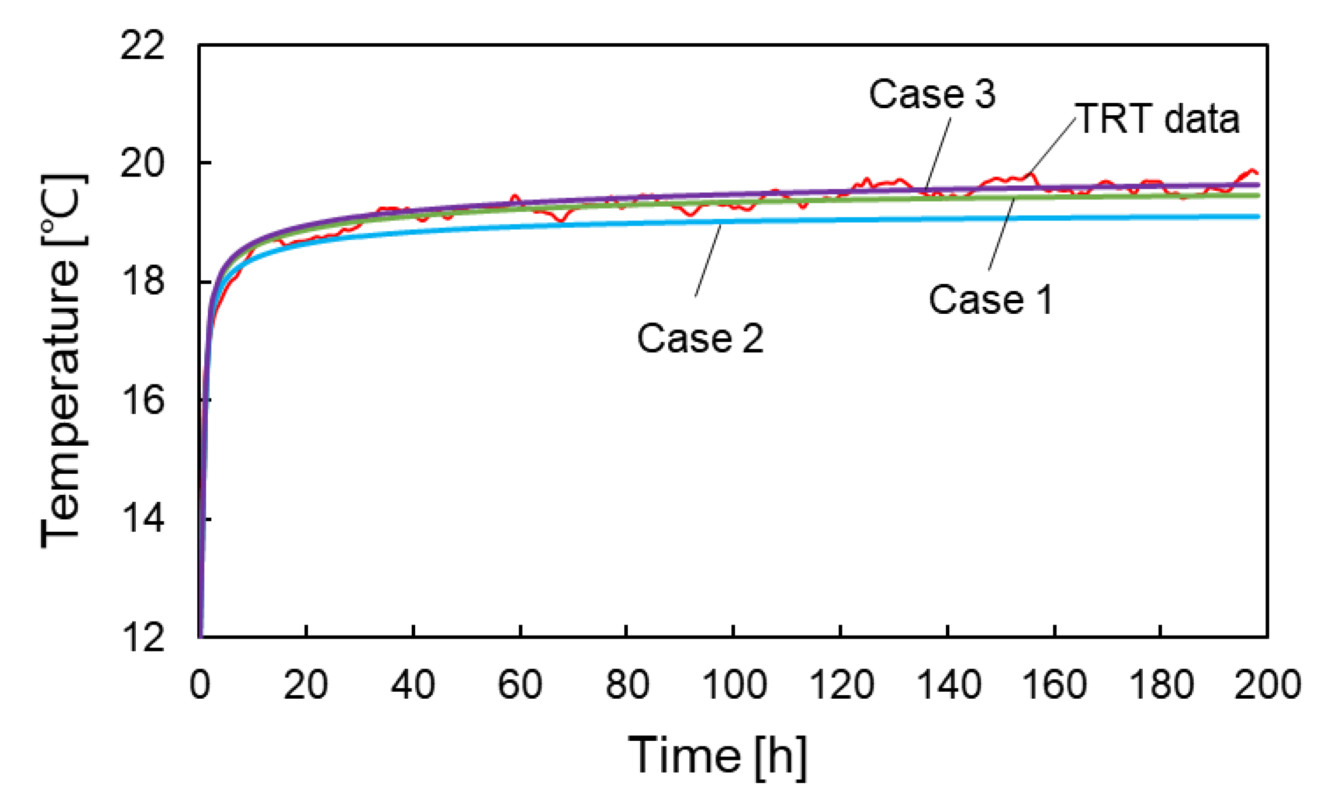
To validate the proposed method, the calculated temperatures were compared with the TRT data. These results were calculated by using the MLS model with the estimated parameters in Equations (10)–(12). Figure 11 shows the temperature change of the calculated results and the TRT data. The calculated results matched well with the TRT data for 198. The comparison results validated the estimated design parameters:
5.2. Analysis Results of Thermal Parameters According to TRT End Time
The TRT is generally operated within a limited time owing to the required construction time and cost. For this reason, the TRT data for 60 h [40], 48 h [21], and 96 h [41] was used to estimate the and after the determination of the zone. The estimated parameters from the proposed method were validated by comparing the TRT data for 200 h. Figure 12 shows the temperature change according to the design parameters determined by the end time of the TRT, which was referred from previous studies: 60 h [40] (Case 1), 48 h [21] (Case 2), and 96 h [41] (Case 3). Table 2 indicates the results for each case. The temperature increments were calculated based on the heat exchange rates of each sublayer. These heat exchange rates were determined by the measured temperature, which might contain measurement errors or be affected by the surrounding environment. Nevertheless, the heat exchange rate converged gradually as the TRT progressed. Based on the estimated thermal parameter at each end time, the temperature results of Cases 1 and 3 were similar but differed slightly from those of Case 2, compared with the measurement data from the DTS. For this reason, the heat exchange rate converged over time. Although a longer TRT time can provide more accurate design parameters, increased construction time and effort are required. Because the optimal TRT time depends on the test location, future studies will be performed to determine the optimal TRT time based on the TRT results of other sites.
5.3. Long-Term Simulation Results According to Time-Variable Building Load
The estimated design parameters were validated through a comparison between the measured data and the calculated results for the long-term period. The measured data above were those of the circulating fluid when the GSHP system was operated with four BHEs (the GSHP system and the target building are described in Section 2). The measured period was from 1 November 2017 to 22 October 2019. The temperature change in the circulating fluid is calculated by using the GSHP simulation tool applied to the estimated parameters and the time-variable building loads as the input parameters. The GSHP simulation was “Ground Club,” developed by Hokkaido University [42]. The simulation tool can incorporate the effects of groundwater flow as well as the multiple BHEs in multilayers [43,44,45].
Figure 13 shows the heating and cooling load of the target building. These building loads were calculated using the electric power consumption of the heat pump and the heat extraction and injection of the BHEs based on Equations (13) and (14). The annual heating and cooling loads were 106.6 and 20.1 GJ from 2017 to 2018, respectively, and 108.7 and 18.1 GJ from 2018 to 2019, respectively. The maximum, minimum, and average outdoor temperatures of the test site (Figure 13b) were 35.6 °C, −18.4 °C, and 9.6 °C, respectively:
Figure 14 shows the average temperatures of the circulating fluid. These temperatures were those measured from the inlet and outlet of the heat pump and the calculated results of the simulation tool. The annual temperature error between the calculated results and the measured data was 6.4% for two years. These comparison results demonstrated the appropriateness of the estimated design parameters for designing the GSHP systems. Table 3 presents the uncertainties of the measured and evaluated parameter in the experimental estimation of the heat transfer rate.
6. Estimation of the Circulating Fluid According to the Borehole Size
The proposed method has the advantage of the consideration for the optimal BHE size in the areas where the groundwater flows rapidly in the specific layers. The conventional TRT analysis methods or the previous research [23] can provide only the weight-average values of the effective thermal conductivity and the groundwater velocity with respect to the depth of the BHE where the TRT was carried out. If the BHE size was changed, the estimated values from the TRT could not use it for the design of the BHE. However, the proposed methodology could provide the effective thermal conductivities and the groundwater velocities in multi-layer. In particular, it is possible to effectively design a BHE size by grasping the thermal properties of the zones and the groundwater velocities. The following paragraph presents the comparison results between the conventional TRT analysis method and the proposed method. Table 4 shows the estimated parameter values according to the TRT analysis methods.
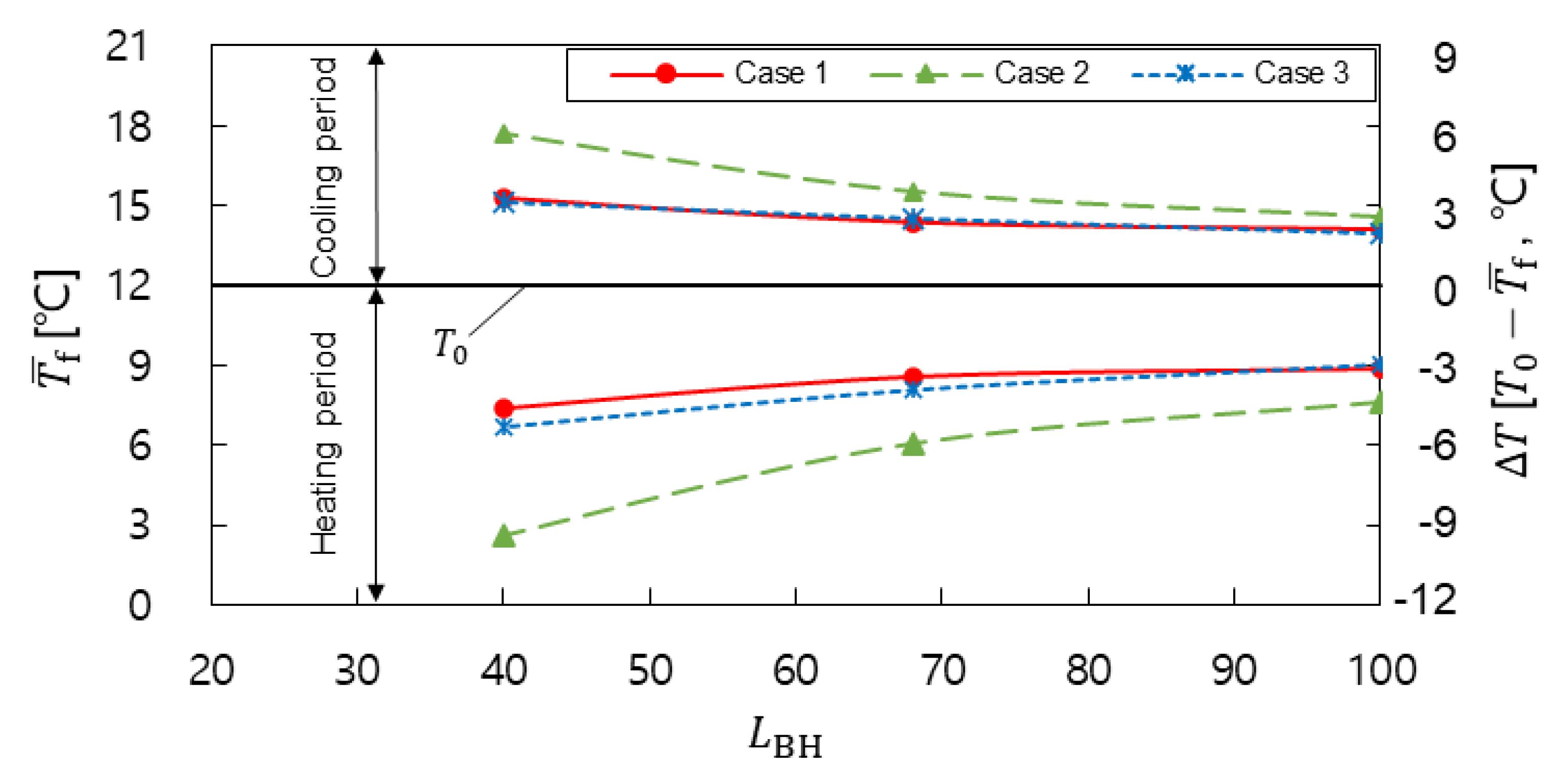
Figure 15 shows that the average temperature of the circulating fluid during the heating and cooling seasons according to the borehole size. in the condition of Case 1 decreased by −3.14 °C from during the heating season. Meanwhile, in the condition of Case 2 decreased by −4.42 °C from during the heating season. This difference shows the importance considering the groundwater flow effects in the TRT analysis method. If the BHEs are designed based on the conventional TRT analysis result (Case 2), more BHEs are required to supply the appropriate temperature of the fluid entering the heat pump to operate the GSHP system. Meanwhile, in the condition of Case 1 decreased by −4.61 °C from despite the BHEs of 100 m being reduced to that of 40 m. This result was obtained because was calculated using the finite cylinder source model and the parameters of Zone 1 in the condition of Case 1 was considered. Zone 1 in the condition of Case 1 was located from the ground surface to −40 m below ground and the of Zone 1 was 2750 m/y. By contrast, in the condition of Case 2 decreased by −9.36 °C when the length of the BHEs was reduced by 40% from 100 m.
Figure 16 shows the average temperature variations of the circulating fluid. These temperatures were calculated for two years based on the conditions of Cases 1-1 and 2-1. The heating and cooling loads were of the same condition as that of the target building described in Section 5.3. The temperature variation in the condition of Case 2-1 exhibited larger fluctuations of −2.7 °C to 1.9 °C compared with that in the condition of Case 1-1.
Figure 17 shows the average temperature variations of the circulating fluid. The condition of Case 3-1 was obtained from a previous study [23], which provided the values of and in a single layer of a 100 m BHE at the same test site. The result shows that the temperature error between Cases 1-1 and 3-1 was 0.3%. Both methods were regarded as suitable for the design of BHEs in areas with rapid groundwater flows. Meanwhile, Figure 18 shows the average temperature variations of the circulating fluid when the borehole size was 40 m. The temperature variation in the condition of Case 3-3 exhibited larger fluctuations of −3.0 °C to 1.8 °C compared with that in the condition of Case 1-3. The seasonal temperature error in the heating season was 9.2%. The proposed method obtained layers with strong groundwater flow effects and provided the temperature variation prediction of the circulating fluid according to the BHE size. It was effective in designing the appropriate BHE size.
7. Conclusions
A TRT analytical method was proposed herein to estimate the groundwater velocity and the effective thermal conductivity of geological zones. Furthermore, the RTT was applied to determine the zone depths by considering the temperature recovery during the relaxation period (Section 3.2 and Section 4.2). Temperature increments at the TRT end time were calculated according to the groundwater velocities using the MLS model (Section 3.2 and Section 4.3). These results were compared with the average temperature increments measured from each zone and its best-fitting value yielded the groundwater velocities. The groundwater velocity was estimated to be 2750, 58, and 0 , whereas the effective thermal conductivity was evaluated to be 2.4, 2.4, and 2.1 for Zones 1, 2 and 3, respectively (Section 4.3).
These estimated velocities and other parameters were applied to the simulation tool to calculate the temperatures of the circulating fluid. The calculated temperatures were validated by comparing them to the measurement data of the circulating fluid in the target building. The annual temperature error between the calculated results and the measured data was 6.4% (Section 5.3). In addition, the seasonal average temperatures of the circulating fluid were estimated according to the BHE size by applying them to the parameters estimated using the TRT analysis methods (Section 6). It was discovered that the proposed method was effective in obtaining layers that were significantly affected by the groundwater flow and demonstrated the appropriate BHE size. The long-term performance can be predicted well using the groundwater velocity and the effective thermal conductivity for each zone obtained from the proposed method as the calculating condition.
Author Contributions
H.C., K.N. drafted the work, conceived and designed the experiments; Y.S. and T.K. (Takeshi Kondo) performed the experiments, and A.A.S. analyzed the data. K.N and T.K. (Takao Katsura) gave the final approval of the version to be published. All authors have read and agreed to the published version of the manuscript.
Funding
This research is a part of the project in New Energy and Industrial Technology Development Organization (NEDO, No. 14101575-0) and is the project results collaborated with Hokkaido University and Tohoku Electric Power Co., Inc.
Acknowledgments
The authors are grateful to the staff who work in the Tohoku Electric Power Co., Inc. for providing us an opportunity to measure and analyze the field data of the GSHP system.
Conflicts of Interest
The authors declare no conflict of interest.
Nomenclature
| volumetric heat capacity () | |
| specific heat capacity () | |
| diameter () | |
| electric power consumption [kW] | |
| heat injection () | |
| heat injection rate () | |
| temperature gradient over the logarithmic time () | |
| depth () | |
| flow rate () | |
| the number of zones | |
| radius () | |
| borehole thermal resistance () | |
| temperature (°C) | |
| mean temperature (°C) | |
| dimensionless temperature | |
| time () | |
| relaxation time of temperature, RTT () | |
| time at stopping the heat supply (h) | |
| effective fluid velocity () | |
| Darcy velocity () | |
| Shank spacing from the center of the pipe to the center of the borehole | |
| Greek letters | |
| thermal diffusivity () | |
| integration parameter | |
| density () | |
| thermal conductivity () | |
| polar angle () | |
| Euler’s constant, (0.5772) | |
| Subscripts | |
| initial value | |
| cooling | |
| fluid | |
| borehole | |
| effective | |
| heating | |
| heat pump | |
| inside | |
| layer | |
| outside | |
| pipe | |
| soil | |
| water | |
| Zone | |
References
- Ozgener, O.; Hepbasli, A.; Ozgener, L. A parametric study on the exergoeconomic assessment of a vertical ground-coupled (geothermal) heat pump system. Build. Environ. 2007, 42, 1503–1509. [Google Scholar] [CrossRef]
- Ozgener, O.; Hepbasli, A. Performance analysis of a solar-assisted ground-source heat pump system for greenhouse heating: An experimental study. Build. Environ. 2005, 40, 1040–1050. [Google Scholar] [CrossRef]
- Nam, Y.; Ooka, R.; Hwang, S. Development of a numerical model to predict heat exchange rates for a ground-source heat pump system. Energy Build. 2008, 40, 2133–2140. [Google Scholar] [CrossRef]
- Carotenuto, A.; Marotta, P.; Massarotti, N.; Mauro, A.; Normino, G. Energy piles for ground source heat pump applications: Comparison of heat transfer performance for different design and operating parameters. Appl. Therm. Eng. 2017, 124, 1492–1504. [Google Scholar] [CrossRef]
- Nam, Y.; Chae, H.B. Numerical simulation for the optimum design of ground source heat pump system using building foundation as horizontal heat exchanger. Energy 2014, 73, 933–942. [Google Scholar] [CrossRef]
- Choi, J.C.; Lee, S.R.; Lee, D.S. Numerical simulation of vertical ground heat exchangers: Intermittent operation in unsaturated soil conditions. Comput. Geotech. 2011, 38, 949–958. [Google Scholar] [CrossRef]
- Mogensen, P. Fluid to duct wall heat transfer in duct system heat storages. Doc. Swed. Counc. Build. Res. 1983, 16, 652–657. [Google Scholar]
- Carslaw, H.S.; Jeager, J.C. Conduction of Heat in Solids; Oxford University Press: Oxford, UK, 1959. [Google Scholar]
- Signorelli, S.; Bassetti, S.; Pahud, D.; Kohl, T. Numerical evaluation of thermal response tests. Geothermics 2007, 36, 141–166. [Google Scholar] [CrossRef]
- Fossa, M.; Rolando, D.; Pasquier, P. Pulsated thermal response test experiment and modelling for ground thermal property estimation. In Proceedings of the IGSHPA Research, Stockholm, Sweden, 18–20 September 2018. [Google Scholar]
- Angelotti, A.; Alberti, L.; la Licata, I.; Antelmi, M. Energy performance and thermal impact of a Borehole Heat Exchanger in a sandy aquifer: Influence of the groundwater velocity. Energy Convers. Manag. 2014, 77, 700–708. [Google Scholar] [CrossRef]
- Choi, J.C.; Park, J.; Lee, S.R. Numerical evaluation of the effects of groundwater flow on borehole heat exchanger arrays. Renew. Energy 2013, 52, 230–240. [Google Scholar] [CrossRef]
- Hecht-Méndez, J.; De Paly, M.; Beck, M.; Bayer, P. Optimization of energy extraction for vertical closed-loop geothermal systems considering groundwater flow. Energy Convers. Manag. 2013, 66, 1–10. [Google Scholar] [CrossRef]
- Lee, C.K.; Lam, H. A modified multi-ground-layer model for borehole ground heat exchangers with an inhomogeneous groundwater flow. Energy 2012, 47, 378–387. [Google Scholar] [CrossRef]
- Wang, H.; Qi, C.; Du, H.; Gu, J. Thermal performance of borehole heat exchanger under groundwater flow: A case study from Baoding. Energy Build. 2009, 41, 1368–1373. [Google Scholar] [CrossRef]
- Wagner, V.; Blum, P.; Kübert, M.; Bayer, P. Analytical approach to groundwater-influenced thermal response tests of grouted borehole heat exchangers. Geothermics 2013, 46, 22–31. [Google Scholar] [CrossRef]
- Spitler, J.D.; Yavuzturk, C.; Rees, S.J. Development of an insitu system and analysis procedure for measuring ground thermal properties. In Proceedings of the Terrastock, Stuttgart, Germany, 28 August–1 September 2000. [Google Scholar]
- Smith, M.; Perry, R. In situ testing and thermal conductivity testing. In Proceedings of the 1999 GeoExchange Technical Conference and Expo, Oklahoma, OK, USA, 16–19 May 1999. [Google Scholar]
- Kavanaugh, S.P.; Xie, L.; Martin, C. Investigation of methods for determining soil and rock formation thermal properties from short-term field tests. Final Report ASHRAE TRP-1118. 2000. Available online: https://www.techstreet.com/standards/rp-1118-investigation-of-methods-for-determining-soil-and-rock-formation-thermal-properties-from-short-term-field-tests?product_id=1711876 (accessed on 14 May 2020).
- Gehlin, S.E.A.; Hellström, G. Comparison of four models for thermal response test evaluation. ASHRAE Trans. 2003, 109, 131–142. [Google Scholar]
- American Society of Heating, Refrigerating and Air-Conditioning Engineers. ASHRAE Handbook–HVAC Applications; American Society of Heating, Refrigerating and Air-Conditioning Engineers, Inc.: Atlanta, GA, USA, 2011. [Google Scholar]
- Wagner, V.; Bayer, P.; Bisch, G.; Kübert, M. Hydraulic characterization of aquifers by thermal response testing: Validation by large-scale tank and field experiments. Water Resour. Res. 2014, 50, 71–85. [Google Scholar] [CrossRef]
- Chae, H.; Nagano, K.; Sakata, Y.; Katsura, T.; Kondo, T. Estimation of fast groundwater flow velocity from thermal response test results. Energy Build. 2020, 206, 109571. [Google Scholar] [CrossRef]
- Sakata, Y.; Katsura, T.; Nagano, K. Multilayer-concept thermal response test: Measurement and analysis methodologies with a case study. Geothermics 2018, 71, 178–186. [Google Scholar] [CrossRef]
- Sakata, Y.; Katsura, T.; Nagano, K.; Ishizuka, M. Field analysis of stepwise effective thermal conductivity along a borehole heat exchanger under artificial conditions of groundwater flow. Hydrology 2017, 4, 21. [Google Scholar] [CrossRef] [Green Version]
- Kallio, J.; Leppäharju, N.; Martinkauppi, I.; Nousiainen, M. Geoenergy research and its utilization in Finland. Geol. Surv. Finl. 2011, 49, 179–185. [Google Scholar]
- Fujii, H.; Okubo, H.; Nishi, K.; Itoi, R.; Ohyama, K.; Shibata, K. An improved thermal response test for U-tube ground heat exchanger based on optical fiber thermometers. Geothermics 2009, 38, 399–406. [Google Scholar] [CrossRef]
- Günzel, U.; Wilhelm, H. Estimation of the in-situ thermal resistance of a borehole using the Distributed Temperature Sensing (DTS) technique and the Temperature Recovery Method (TRM). Geothermics 2000, 29, 689–700. [Google Scholar] [CrossRef]
- Freifeld, B.; Finsterle, S.; Onstott, T.C.; Toole, P.; Pratt, L.M. Ground surface temperature reconstructions: Using in situ estimates for thermal conductivity acquired with a fiber-optic distributed thermal perturbation sensor. Geophys. Res. Lett. 2008, 35, 3–7. [Google Scholar] [CrossRef] [Green Version]
- McDaniel, A.; Tinjum, J.M.; Hart, D.; Lin, Y.-F.; Stumpf, A.J.; Thomas, L. Distributed thermal response test to analyze thermal properties in heterogeneous lithology. Geothermics 2018, 76, 116–124. [Google Scholar] [CrossRef]
- Saito, T.; Hamamoto, S.; Mon, E.E.; Takemura, T.; Saito, H.; Komatsu, T.; Moldrup, P. Thermal properties of boring core samples from the Kanto area, Japan: Development of predictive models for thermal conductivity and diffusivity. Soils Found. 2014, 54, 116–125. [Google Scholar] [CrossRef] [Green Version]
- Santa, G.D.; Peron, F.; Galgaro, A.; Cultrera, M.; Bertermann, D.; Müller, J.; Bernardi, A. Laboratory measurements of gravel thermal conductivity: An update methodological approach. Energy Procedia 2017, 125, 671–677. [Google Scholar] [CrossRef]
- Hamdhan, I.N.; Clarke, B.G. Determination of thermal conductivity of coarse and fine sand soils. In Proceedings of the World Geothermal Congress, Bali, Indonesia, 25–29 April 2010. [Google Scholar]
- Colangelo, F.; De Luca, G.; Ferone, C.; Mauro, A. Experimental and numerical analysis of thermal and hygrometric characteristics of building structures employing recycled plastic aggregates and geopolymer concrete. Energies 2013, 6, 6077–6101. [Google Scholar] [CrossRef] [Green Version]
- Diao, N.; Li, Q.; Fang, Z. Heat transfer in ground heat exchangers with groundwater advection. Int. J. Therm. Sci. 2004, 43, 1203–1211. [Google Scholar] [CrossRef]
- Eklöf, C.; Gehlin, S. A Mobile Equipment for Thermal Response Test. Master’s Thesis, Lulea University of Technology, Lulea, Sweden, 1996. [Google Scholar]
- Raymond, J.; Therrien, R.; Gosselin, L.; Lefebvre, R. A review of thermal response test analysis using pumping test concepts. Ground Water 2011, 49, 932–945. [Google Scholar] [CrossRef]
- Yavuzturk, C.; Spitler, J.D. Short time step response factor model for vertical ground loop heat exchangers. ASHRAE Trans. 1999, 105, 475–485. [Google Scholar]
- Choi, W.; Ooka, R. Interpretation of disturbed data in thermal response tests using the infinite line source model and numerical parameter estimation method. Appl. Energy 2015, 148, 476–488. [Google Scholar] [CrossRef]
- Nagano, K. Standard Procedure of Standard TRT, Version 2.0; Heat Pump and Thermal Storage Technology Center of Japan: Tokyo, Japan, 2011. [Google Scholar]
- Lamarche, L.; Raymond, J.; Pambou, C.H.K. Evaluation of the internal and borehole resistances during thermal response tests and impact on ground heat exchanger design. Energies 2017, 11, 38. [Google Scholar] [CrossRef] [Green Version]
- Nagano, K.; Katsura, T.; Takeda, S. Development of a design and performance prediction tool for the ground source heat pump system. Appl. Therm. Eng. 2006, 26, 1578–1592. [Google Scholar] [CrossRef]
- Katsura, T.; Nagano, K.; Takeda, S. Method of calculation of the ground temperature for multiple ground heat exchangers. Appl. Therm. Eng. 2008, 28, 1995–2004. [Google Scholar] [CrossRef]
- Katsura, T.; Nagano, K.; Narita, S.; Takeda, S.; Nakamura, Y.; Okamoto, A. Calculation algorithm of the temperatures for pipe arrangement of multiple ground heat exchangers. Appl. Therm. Eng. 2009, 29, 906–919. [Google Scholar] [CrossRef]
- Katsura, T.; Nagano, K.; Takeda, S.; Shimakura, K. Heat transfer experiment in the ground with ground water advection. Proceedings of 10th Energy Conservation Thermal Energy Storage Conference Ecostock, Stockton, NJ, USA, May 31–June 2 2006. [Google Scholar]
Figure 1.
Site description: (a) the ground plan of the test site; (b) the geological column section.
Figure 1.
Site description: (a) the ground plan of the test site; (b) the geological column section.
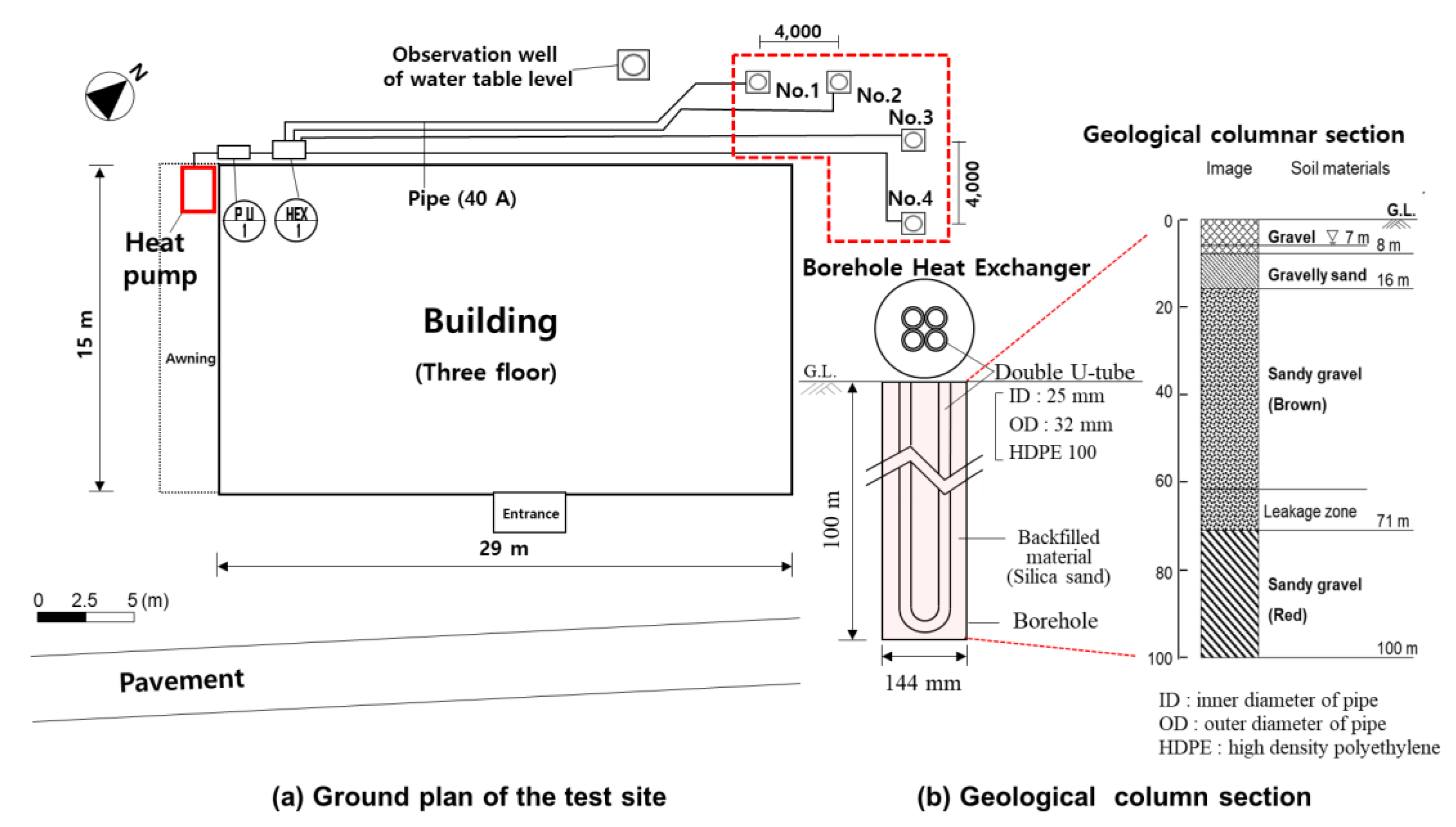
Figure 2.
Schematics of the thermal response test (TRT) machine units and the borehole heat exchangers (BHEs).
Figure 2.
Schematics of the thermal response test (TRT) machine units and the borehole heat exchangers (BHEs).
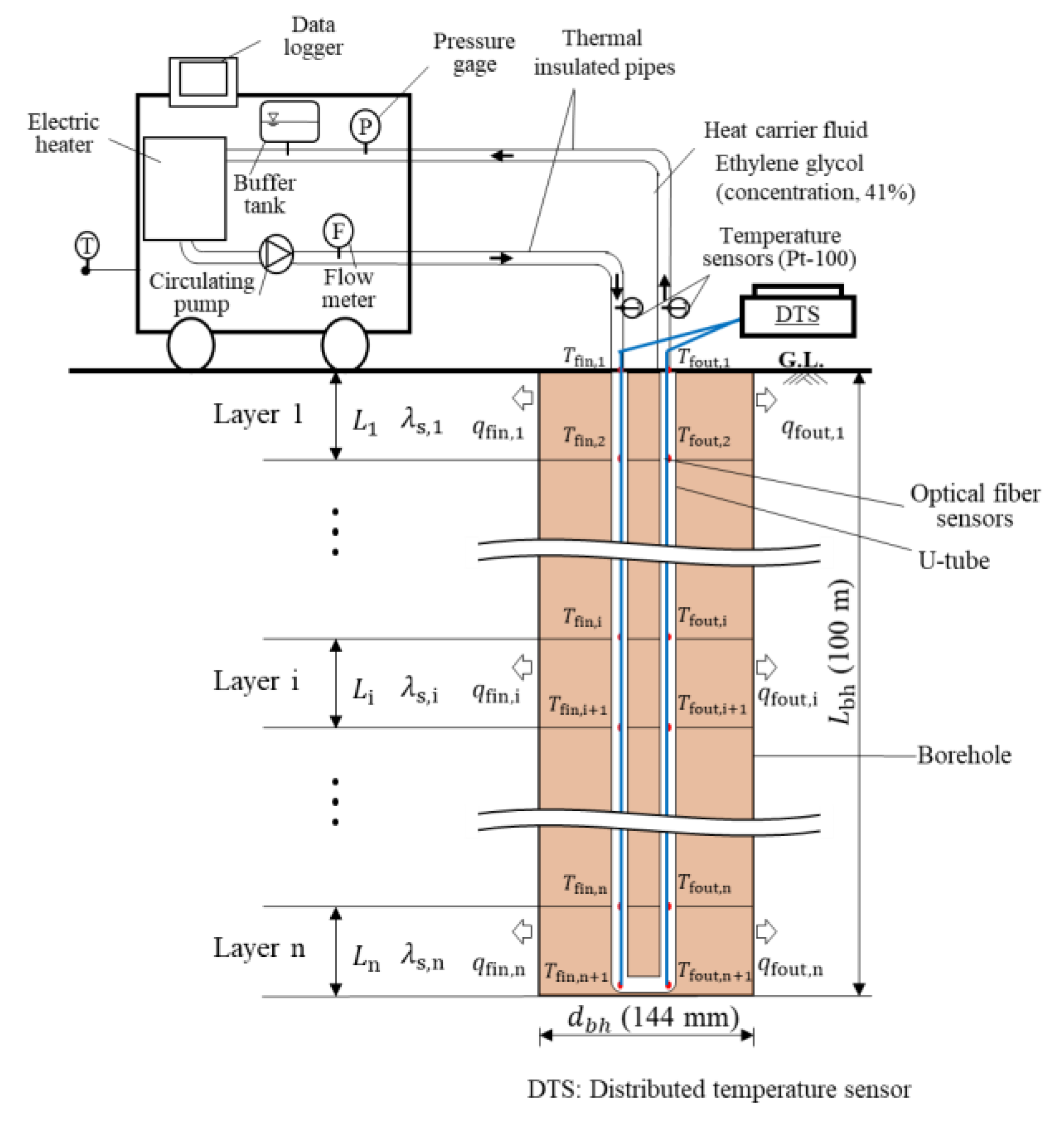
Figure 3.
Relationship between the dimensionless temperature and the dimensionless relaxation time of temperature (RTT); (a) dimensionless temperature variation (b) dimensionless RTT according to the groundwater velocity.
Figure 3.
Relationship between the dimensionless temperature and the dimensionless relaxation time of temperature (RTT); (a) dimensionless temperature variation (b) dimensionless RTT according to the groundwater velocity.
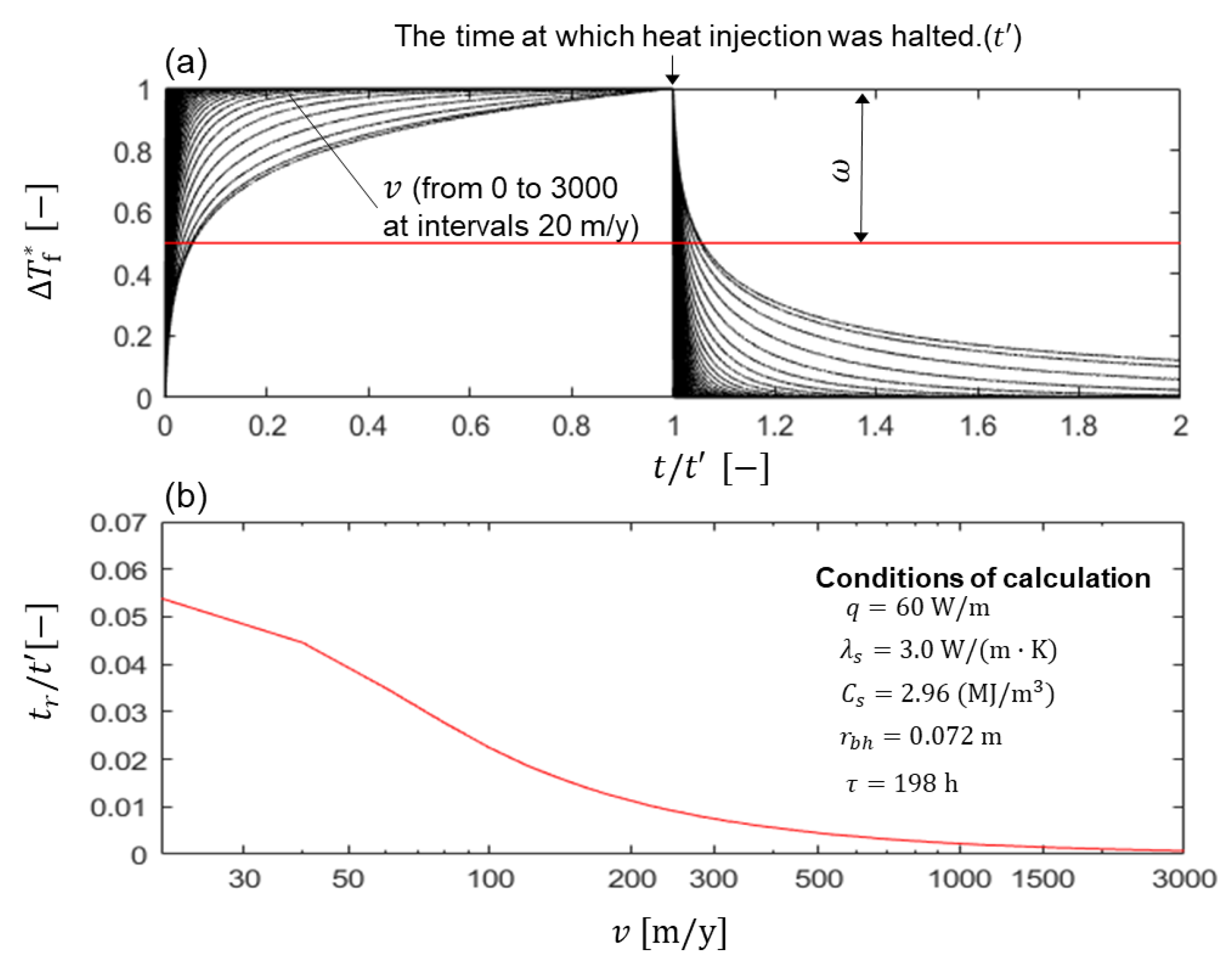
Figure 4.
Flow chart of the calculation.

Figure 5.
Measurement data of the TRT: (a) the temperature data of the inlet and outlet; and the average temperature of the Pt-100 sensors; (b) the heat injection and flow rate.
Figure 5.
Measurement data of the TRT: (a) the temperature data of the inlet and outlet; and the average temperature of the Pt-100 sensors; (b) the heat injection and flow rate.
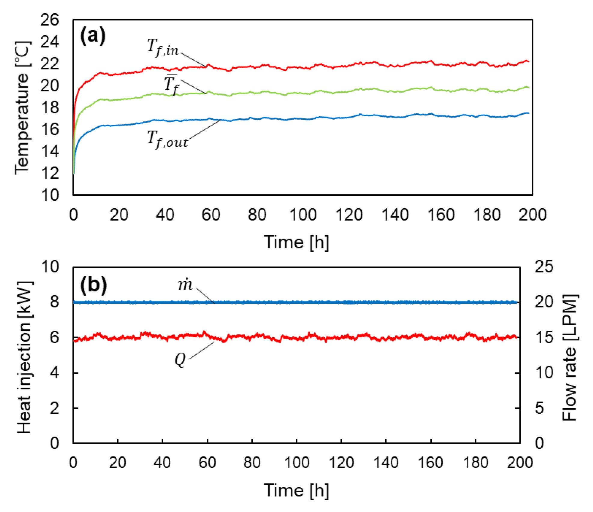
Figure 6.
Dimensionless temperature variation and the RTT of the measurement data and the calculated results.
Figure 6.
Dimensionless temperature variation and the RTT of the measurement data and the calculated results.

Figure 7.
RTT according to the groundwater velocity.

Figure 8.
Vertical distribution of the RTT.

Figure 9.
(a) Vertical temperature distribution during the heat injection period, and (b) the heat transfer rate of each zone.
Figure 9.
(a) Vertical temperature distribution during the heat injection period, and (b) the heat transfer rate of each zone.
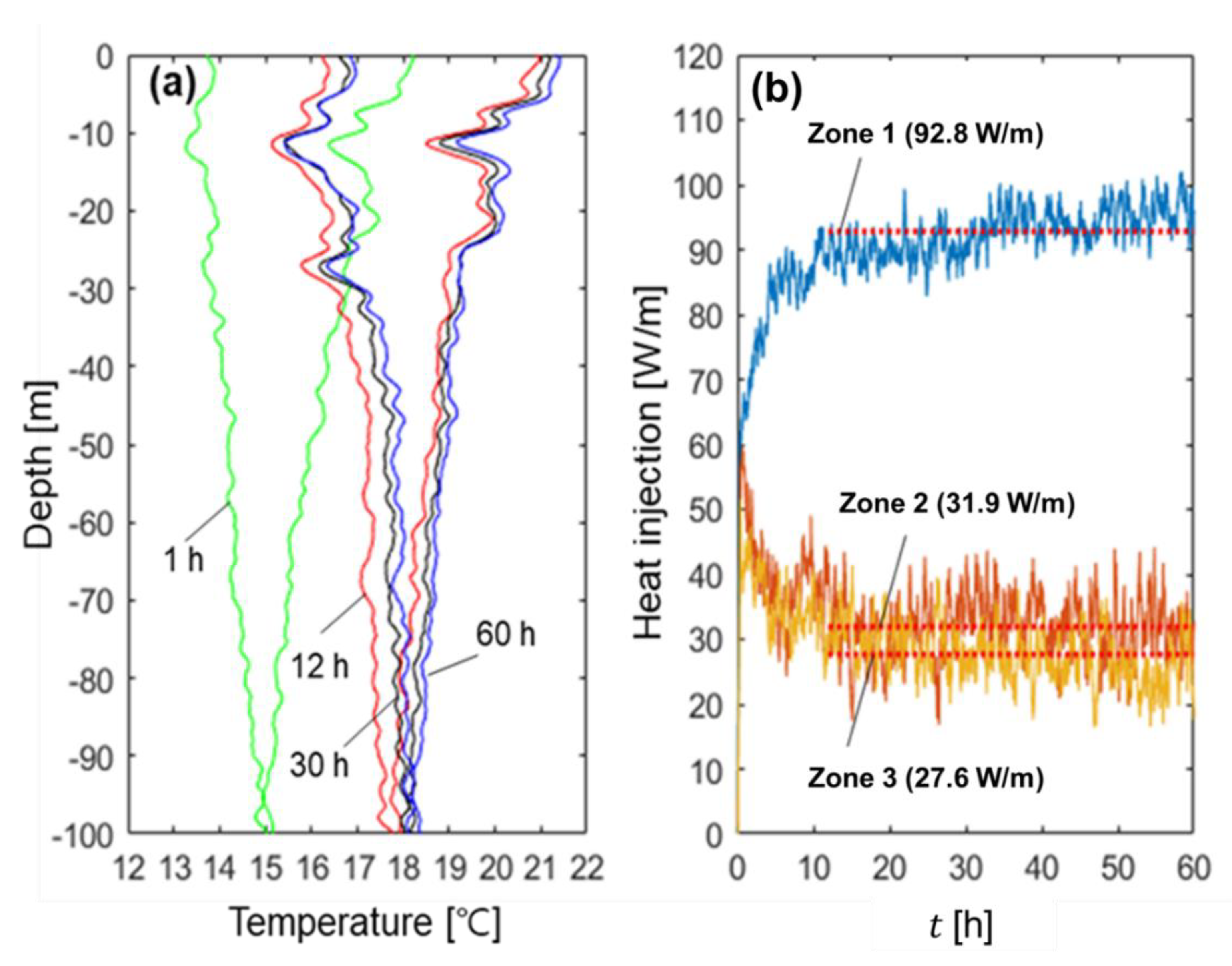
Figure 10.
Temperature increment according to the heat exchanger rate and the groundwater velocity at the end of the TRT; (a) Zone 1, (b) Zone 2 and (c) Zone 3.
Figure 10.
Temperature increment according to the heat exchanger rate and the groundwater velocity at the end of the TRT; (a) Zone 1, (b) Zone 2 and (c) Zone 3.
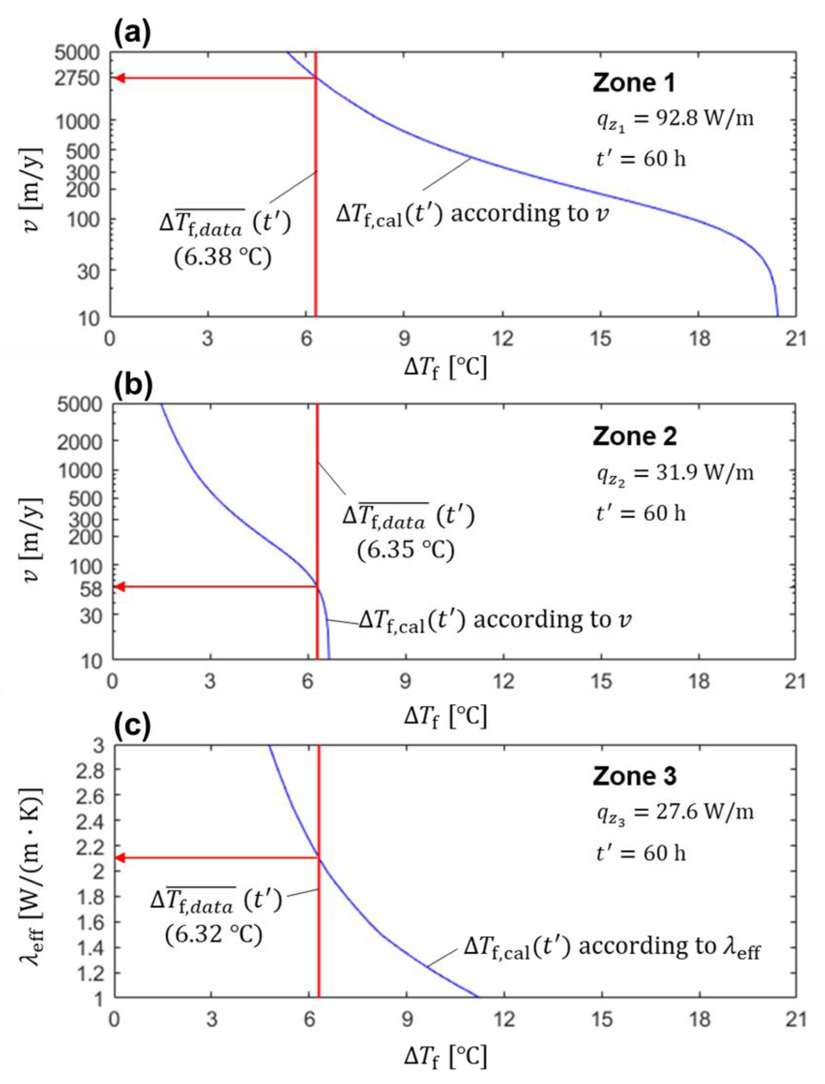
Figure 11.
Comparison between the calculated results and the TRT data.
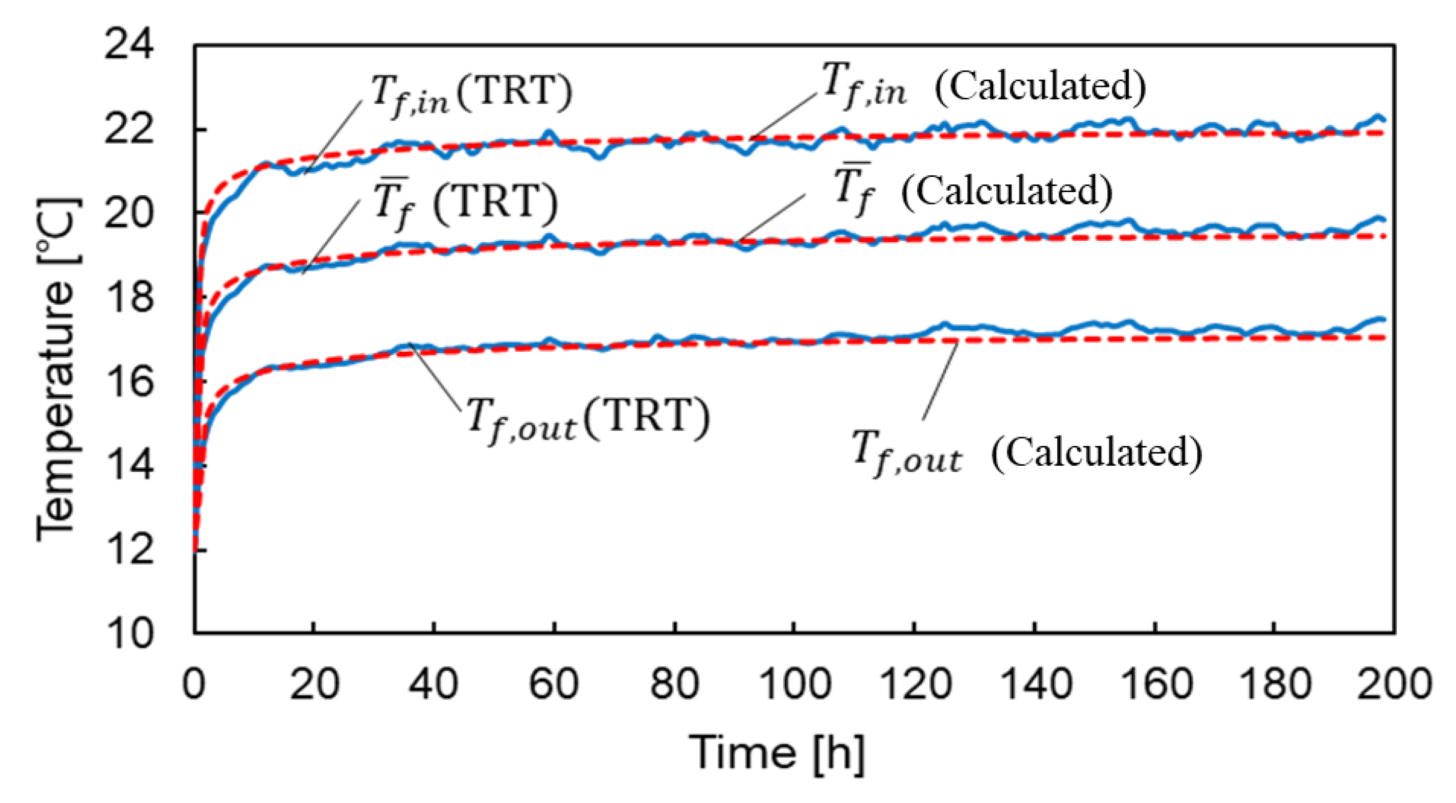
Figure 12.
Temperature variation according to the TRT end time.

Figure 13.
Heating and cooling load of the target building; (a) building load and (b) outdoor temperature.
Figure 13.
Heating and cooling load of the target building; (a) building load and (b) outdoor temperature.
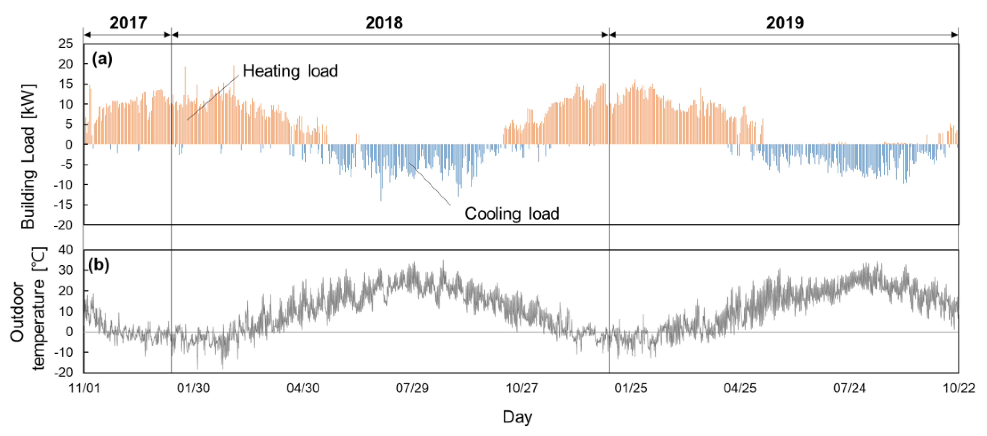
Figure 14.
Average temperatures of the circulating fluid: (a) two years for the heating and cooling; (b) the representative three days for the heating period; (c) the representative three days for the cooling period.
Figure 14.
Average temperatures of the circulating fluid: (a) two years for the heating and cooling; (b) the representative three days for the heating period; (c) the representative three days for the cooling period.

Figure 15.
Average temperature of the circulating fluid during the heating and cooling seasons according to the borehole size.
Figure 15.
Average temperature of the circulating fluid during the heating and cooling seasons according to the borehole size.

Figure 16.
Average temperature variation of the circulating fluid; comparison between the proposed method and the conventional TRT analysis method.
Figure 16.
Average temperature variation of the circulating fluid; comparison between the proposed method and the conventional TRT analysis method.
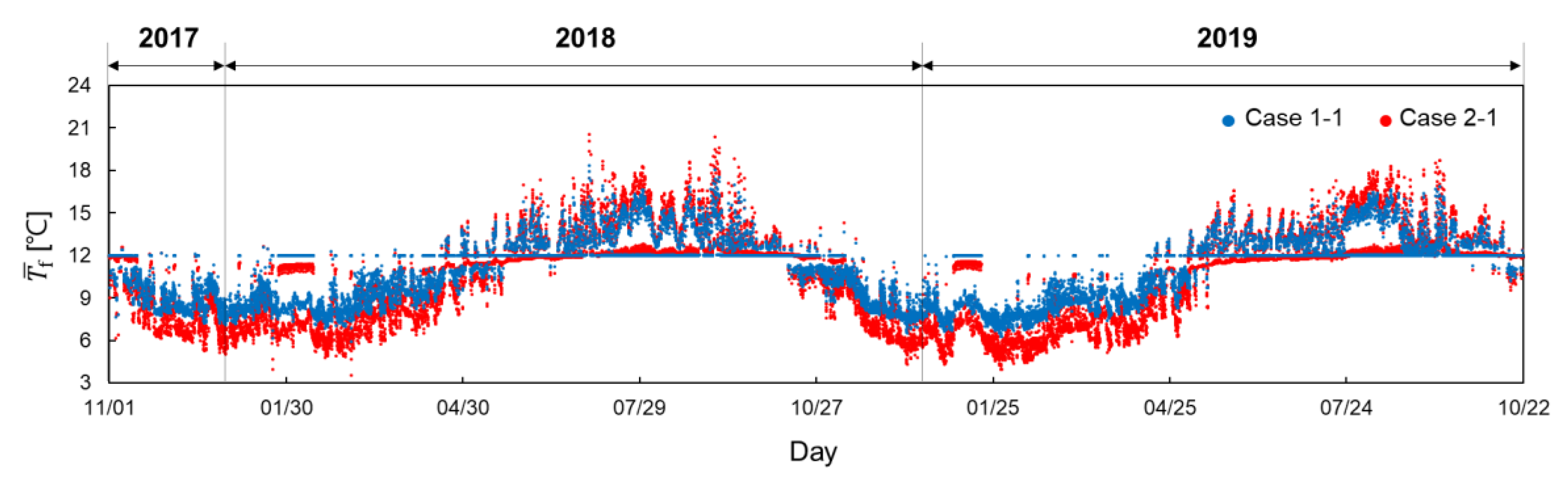
Figure 17.
Average temperature variation of the circulating fluid; comparison between the multilayer and single layer for the design parameters.
Figure 17.
Average temperature variation of the circulating fluid; comparison between the multilayer and single layer for the design parameters.
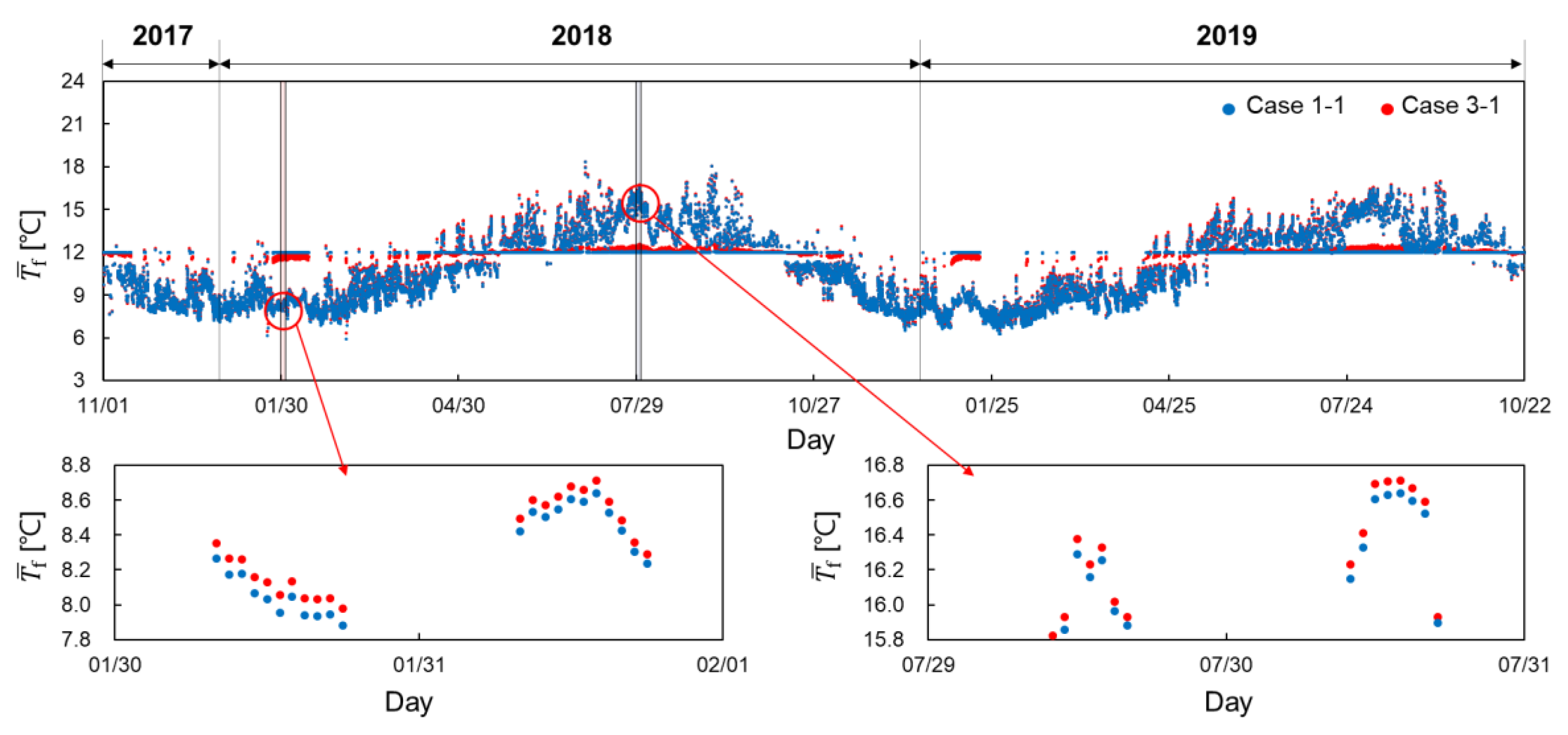
Figure 18.
Average temperature variation of the circulating fluid; comparison between the multilayer and the single layer for the design parameters for the borehole depth of 40 m.
Figure 18.
Average temperature variation of the circulating fluid; comparison between the multilayer and the single layer for the design parameters for the borehole depth of 40 m.


Table 1.
Conditions of the zones.
| Layer | |||
|---|---|---|---|
| Zone 1 | 0–40 | ||
| Zone 2 | 40–68 | ||
| Zone 3 | 68–100 |
Table 2.
Results of the thermal parameter according to the end time.
| Case | Case 1 (End Time = 60 h) | Case 2 (End Time = 48 h) | Case 3 (End Time = 96 h) | |
|---|---|---|---|---|
| Zone 1 | [) | 92.8 | 91.8 | 94 |
| ) | 2.4 | 2.4 | 2.13 | |
| ) | 2750 | 3250 | 2730 | |
| Zone 2 | ) | 31.9 | 32.1 | 31.1 |
| ) | 2.4 | 2.4 | 2.36 | |
| ) | 58 | 89 | 28 | |
| Zone 3 | ) | 27.6 | 28.4 | 26.1 |
| ) | 2.1 | 2.36 | 1.97 | |
| ) | 0 | 0 | 0 | |
Table 3.
Measurement uncertainty in the measured and the evaluated parameters.
| Parameter | Measurement Uncertainty |
|---|---|
| ) | |
| ) | |
| ) | |
| ) | |
| ) |
Table 4.
Estimated parameter values according to the TRT analysis methods.
| Case | ||||
|---|---|---|---|---|
| Case 1 (proposed method) | Case 1-1 (three zones) | 100 (40/28/32) | 2.4/2.4/2.1 | 2750/58/0 |
| Case 1-2 (two zones) | 68 (40/28) | 2.4/2.4 | 2750/58 | |
| Case 1-3 (one zone) | 40 | 2.4 | 2750 | |
| Case 2 (conventional TRT analysis method) | Case 2-1 | 100 | 9.5 | 0 |
| Case 2-2 | 68 | 9.5 | 0 | |
| Case 2-3 | 40 | 9.5 | 0 | |
| Case 3 (previous research [23]) | Case 3-1 | 100 | 4.7 | 120 |
| Case 3-2 | 68 | 4.7 | 120 | |
| Case 3-3 | 40 | 4.7 | 120 | |
© 2020 by the authors. Licensee MDPI, Basel, Switzerland. This article is an open access article distributed under the terms and conditions of the Creative Commons Attribution (CC BY) license (http://creativecommons.org/licenses/by/4.0/).
Share and Cite
MDPI and ACS Style
Chae, H.; Nagano, K.; Sakata, Y.; Katsura, T.; Serageldin, A.A.; Kondo, T. Analysis of Relaxation Time of Temperature in Thermal Response Test for Design of Borehole Size. Energies 2020, 13, 3297. https://doi.org/10.3390/en13133297
AMA Style
Chae H, Nagano K, Sakata Y, Katsura T, Serageldin AA, Kondo T. Analysis of Relaxation Time of Temperature in Thermal Response Test for Design of Borehole Size. Energies. 2020; 13(13):3297. https://doi.org/10.3390/en13133297
Chicago/Turabian StyleChae, Hobyung, Katsunori Nagano, Yoshitaka Sakata, Takao Katsura, Ahmed A. Serageldin, and Takeshi Kondo. 2020. "Analysis of Relaxation Time of Temperature in Thermal Response Test for Design of Borehole Size" Energies 13, no. 13: 3297. https://doi.org/10.3390/en13133297
Note that from the first issue of 2016, this journal uses article numbers instead of page numbers. See further details here.