Abstract
Renewable Energy Sources are becoming widely spread, as they are sustainable and low-carbon emission. They are mostly penetrating the MV Distribution Networks as Distributed Generators, which has determined the evolution of the networks’ control and supervision systems, from almost a complete lack to becoming fully centralized. This paper proposes innovative voltage control architectures for the distribution networks, tailored for different development levels of the control and supervision systems encountered in real life: a Coordinated Control for networks with basic development, and an optimization-based Centralized Control for networks with fully articulated systems. The Centralized Control fits the requirements of the network: the challenging harmonization of the generator’s capability curves with the regulatory framework, and modelling of the discrete control of the On-Load Tap Changer transformer. A realistic network is used for tests and comparisons with the Local Strategy currently specified by regulations. The proposed Coordinated Control gives much better results with respect to the Local Strategy, in terms of loss minimization and voltage violations mitigation, and can be used for networks with poorly developed supervision and control systems, while Centralized Control proves the best solution, but can be applied only in fully supervised and controlled networks.
1. Introduction
The use of Renewable Energy Sources (RESs) is becoming widely spread around the world, as they are sustainable, require low maintenance, and are low-carbon emission resources [1]. As a proof, the European Union has enforced the Renewable Energy Directive 2018/2001/EU [2], where the new overall EU target for RES coverage of total energy demands has been raised to 32% by 2030. Although there are clear benefits of RES, the most notable being environmental impact, a high penetration of renewable Distributed Generators (DGs) in MV Distribution Networks (DN) causes important technical challenges, as it involves a change of paradigm in their operation: they are evolving from passive, demand-only networks to active networks.
Nowadays, the DNs are still managed as passive networks; a limited set of measurements is available at the HV/MV primary Substations level, and some measurements are available for a minor number of DNs at the secondary MV/LV Substations level, while the network is operated mainly through long-term off-line planning and limited real-time HV/MV transformer On-Load Tap Changer (OLTC) control [3]. A high penetration of DGs, though, significantly increases the probability of reverse power flow, and changes the distribution of the voltage profile across the feeder. Instead of continuously dropping from the primary substation, it can take any shape, and cannot be controlled through the HV/MV OLTC transformer alone. In this new context, it is necessary to exploit the DGs through advanced algorithms for automatic real-time operation and control [1]. This also means a remarkable change of DNs from the technical, economic and regulatory points of view: it is expected that distribution companies will assume tasks and responsibilities similar to those undertaken by the Transmission System Operators (TSOs), and hence will become local Distribution System Operators (DSOs).
A high level of real-time observability of the DNs is required for these advanced algorithms, a level that can be achieved only through state estimation algorithms, requiring redundancy, synchronization and statistical characterization of the measured data—a requirement that is not satisfied by the current state of DNs. Moreover, in the short-term, it is difficult to achieve this due to the massive investments required into the necessary equipment. However, things are not staying still, since, the traditional Supervisory Control And Data Acquisition (SCADA) systems are evolving towards advanced architectures and functionalities, making the DN more observable and controllable [4,5,6,7,8,9]. In greater detail, papers [4,5] present the typical Italian context, wherein a basic SCADA architecture is used to monitor the network. This architecture represents the framework for the basic network operation functions: state estimation and voltage control. Paper [4] focuses on SCADA architecture, while paper [5] focuses on the network operation functions. In [6], the latest developments of the architecture and functionalities of [4,5] are introduced. The SCADA is extended, and a Network Calculation Algorithm System is introduced. It contains evolved state estimation and voltage control functions, together with an innovative DG economical dispatch algorithm. At the end, the paper also reports some real-life cases of DNs using the illustrated architecture. Paper [7] is another real-case example where a smart grid architecture is employed, implementing an innovative automatic procedure for selective fault detection, based on logic selectivity and fast network reconfiguration. Paper [8] proposes an automation system logic for DNs, which aims at improving reliability indices through the implementation of selective fault detection, fast network reconfiguration and automatic back-feeding. Paper [9] proposes a series of suitable indicators to quantify the performance of smart grids and, consequently, to define penalties and/or rewards for DSOs. The potential role of these indicators is shown through evaluation of real-life examples. Continuing the exposition, on the other hand, innovative algorithms are being developed to both maximize the observability of the DN, considering the limited number of measurement devices, and to optimize the installation of new ones [10,11,12,13,14,15]. In [10,11], the authors propose innovative state estimation algorithms, designed for the current DN situation. Paper [10] represents a solution for the majority of DNs, as it works only with primary substation measurements, while paper [11] proposes an advanced solution wherein few measurements along the feeders of the DNs are known. Paper [12] presents an algorithm for the real-time estimation of DG production downstream of a primary substation. The algorithm provides real-time estimations to the TSO about the DN status. Papers [13,14,15] consider the optimization of the installation of new measurement devices in the DN, with the goal of minimizing the investments. Paper [13], one of the pioneer works in the field, proposes a technique based on the sequential improvement of a bivariate probability index governing relative errors in voltage and angle estimates at each bus. It employs an iterative mechanism to put a measurement on the location with the largest area of the 2−σ error ellipse, until the relative errors are below the threshold. Papers [14,15] are among the recent developments in the area: paper [14] presents various genetic algorithms to solve the problem, and identifies the best solution, while paper [15] proposes a mixed-integer semidefinite programming model to decide the optimal locations and types of measurement devices to minimize the worst-case estimation errors over different system operating conditions.
Thus, depending on the SCADA evolution level, various innovative algorithms for the automatic real-time operation of DN can be designed, from the simple, with reduced controllability, to the complex, with maximum controllability. This paper focuses on voltage control algorithms, which can be classified into three main groups [16]: (1) Local Control, which relies on local measurements, (2) Coordinated Control, an evolution of Local Control, working with a base telecommunication system, and (3) Centralized Control, which involves the complete observability and controllability of the DN. The goal of voltage control is not only to mitigate voltage limit violations and, implicitly, to increase Hosting Capacity (HC) for DGs, but it also represents a resource for optimizing the DN according to different objectives, such as system losses reduction or power factor optimization.
Significant research can be found in the literature on the three mentioned groups. Local Control uses only locally available information without any information exchange with a centralized control point. Thus, it is the strategy that best fits the contemporary context, wherein many DNs evolve slowly with respect to the historical situation. For this reason, it is already mandated by national standards, e.g., the Italian Technical Committee 316, and the IEC international standard [17]. In this strategy, each DG unit operates individually and is uncoordinated with other devices, leading to contained costs [18]. Like any voltage regulation performed through generating units, the Local Control also exploits the reactive power capability of the DGs. In fact, these generators could be coupled with additional compensators to increase their capability [19]. Static compensators (STATCOM), Distribution STATCOM (D-STATCOM), Static Var Compensators (SVC), fixed capacitor banks and shunt capacitor banks have been investigated in [20,21,22], although some of these devices are costly. In its most general form, Local Control consists of acting on the power factor of the DG unit in order to keep the voltage at the DG terminals in check. In [23], it is shown that the power factor could act on the DN’s voltage profile and increase its HC. Other papers study the combination of various methods with power factor control, in order to gain some advantages such as reliability, efficiency and flexibility [24,25]. Finally, in [26], the authors investigate various local voltage control strategies where the control variable (i.e., DGs power factor or reactive power output, for instance) linearly varies with the controlled/monitored quantity, such as the nodal voltage or real power output. These control laws are designed to comply with the regulatory requirements [17], and the paper identifies the achievements obtainable from all. It is worth noticing that paper [27] warns about the probability that Local Control strategies could cause unwanted voltage fluctuations at the point of common coupling (PCC). A solution is to adopt an incremental Local Control devoted to preserving the dynamic stability of the regulation, e.g., gradient-based techniques. Most notably, paper [28] investigates such an approach where optimization procedures are performed over stochastic scenarios of the grid, with the final goal of identifying the optimal shape of the Local Control. However, the dynamic response of the system is not investigated.
Coordinated Voltage Control (CVC) works with the network’s topology and the electrical parameters of the DN’s feeders, and tries to satisfy operational limits, driving the DN towards a possible optimum. It is suitable for simple networks with few control possibilities and optimization tools, and thus can be considered in simplified forms for poorly supervised large networks with limited telecommunication possibilities. The simplest CVC was studied in [29], and consists of controlling the substation’s voltage, based on the voltage’s lower and upper bounds. A new CVC method with a reactive power management scheme has been studied in [30]. A method that combines reactive power injection by SVC with tap control, using information from sensors across the distribution line, is proposed in [31]. Finally, in [32], real power control is preferred in order to control the voltage. These strategies are limited to small networks, e.g., microgrids, for as long as they are problematic to use in larger scale environments; however, they do not require an increased level of monitoring, data acquisition or controllability of DN.
Other CVC approaches use specialized optimization algorithms to calculate the control variables. The Genetic Algorithm (GA) has been used in [33,34], while the Particle Swarm Optimization (PSO) algorithm in [35]. A new two-stage voltage control scheme for controlling the OLTC, capacitor banks and DGs using micro and recursive GAs has been investigated in [36]. Here, the optimal reactive power generation profile is obtained by minimizing the power losses. The methods used in [33,34,35,36] belong to the class of heuristic optimization algorithms, which present various disadvantages: (1) they require a large number of evaluations of the solution space across many iterations, thus, for large size problems, i.e., large DNs, the computation time could reach high values that are unsuited for real-time applications; (2) they work with a limited number of possible solutions, and so the solution space is often poorly explored. This gives a high probability that different solutions will be obtained for the same starting point; (3) the parameters that configure their functioning (like mutation probability for GAs) are problem- and size-dependent, so it is difficult to find a good general set-up for them. Thus, these types of algorithms are still limited to small and simple cases. Another approach comes from the use of distributed learning methods, i.e., multiagent systems, which have been investigated in [37,38]. However efficient they may be, these methods have a hidden flaw that could jeopardize their implementation: they work optimally when the real operating conditions are similar to those used to train them. Moreover, for large DN networks, optimization approaches require (i) a well-developed monitoring system of the grid, where the measurements are redundant and state estimation can be performed, and (ii) an advanced telecommunication system that allows the full control of the DN in a centralized manner (but under these conditions, the voltage control scheme becomes the Centralized one).
It follows from all the previous considerations that simpler CVC methods are the most proper and robust when it comes to large DNs. Two innovative CVCs, exploiting time domain simulation and statistical DN planning, are discussed in [39]. An electric distance-based approach, that considers structural changes to minimize the operational conflicts, was proposed in [40]. Finally, the importance of reliable communication infrastructure and the quality of service in CVC was discussed in [41].
Centralized Control for DNs is designed with a complete and continuous communication system, which can assure a high degree of observability (where an accurate state-estimation can be performed) and controllability. This step is based on continuous Optimal Reactive Power Flow (ORPF) calculations in the network model, provided by the state estimator, wherein the set points for the voltage control assets (OLTC, DGs, etc.) are optimized and delivered. Then, during continuous operation, the optimal set-points and measured values are compared to optimally adapt the set-points to the current network status.
There are many techniques used for centralized control to formulate different types of objective functions [42,43,44]. In greater detail, [42] proposes objective functions typical of the transmission network, like the classic active power losses minimization and the maximization of the reactive power reserves to keep the system secure in case of N-1 contingencies. Paper [43] extends the set of objective functions with the maximization of the voltage security of the network. On the other hand, paper [44] focuses on objective functions typical to the DNs, like the minimization of the distance between the reactive output of the generators that optimize the network and the user-desired output (in general, zero), or the flattening of the voltage profile of the network around the nominal value. Their advantage consists in providing an optimized solution and, as they have flexibility in defining constraints, effectively handling nonlinear programming. Various ORPF models for DNs are extensively reported in the literature [45,46,47,48]. GA, PSO, Evolutionary PSO, Discrete PSO, sensitivity theory, tabu search, Artificial Neural Network, fuzzy logic, multi agents and gradient-based methods are employed to find the solution to these ORPFs. The disadvantages of the heuristic approaches with regard to real-life implementation were stated earlier. At the same time, gradient-based methods, e.g., interior-point methods, have clear advantages: they are deterministic, since they provide a unique solution and they can converge fast. However, they require the ORPF to be formulated as a continuous non-linear programming (NLP) problem. Unfortunately, OLTC is a discrete control, therefore ORPF becomes a mixed-integer, non-linear programming (MINLP) problem, that, in general, requires a large computation time. This problem is handled in the literature in different ways. In [45], Benders’ decomposition is used; in [46], the MINLP formulation is solved by an approach based on the integration of trust region sequential quadratic programming and branch and bound techniques; paper [47] directly engages an MINLP solver, while paper [48] applies the aforementioned heuristic approaches. While the disadvantages of [47] are already clear, papers [45,46,47] engage complex models without clearly showing the advantages: either small-size networks are used in tests [47], or computation times are not reported [45,47]; in fact, in [46], ORPF is applied to a 19-bus feeder with two DG units, and it converges in about one minute, while in [45,47] ORPF is used as a planning tool rather than a real-time operation tool. Finally, the models proposed in these papers do not consider a subtle but important aspect: the reactive power capability requirements at the PCC of the DG unit with the grid, as specified by regulatory framework [49]. In general, the DG unit is required to guarantee the controllability of the reactive power within a fixed band, or within a band given by a limit power factor, or a combination of the two. Additionally, this requirement can be extended to the interface between the DN and transmission network [50]. The subtility is that they are actually imposed by the regulatory framework, and not by the physics of the generators. While the physical limits are generally wider, the regulatory limits are the ones to be considered by the ORPF. However, these limits could be too tight and not sufficient to mitigate the various constraints of the model, in particular the voltage bounds, leading to the ORPF’s divergence. Thus, it is necessary to model the capability limits with care; to consider the regulatory limits, but allow their relaxation to the physical limits in case of emergency. This mechanism is not considered in any of the investigated papers. Only [45] models the power factor limits, but it models them as a rigid limit.
This paper proposes innovative voltage control strategies, which are designed to be compatible with various stages of the development of supervision and control systems for large DNs: (i) Local Control for DNs that are poorly supervised and lack telecommunication systems; (ii) Coordinated Control for the DNs that are still poorly supervised, but have a base telecommunication system that allows the simple coordination of the reactive power resources; and (iii) Centralized Control for DNs with an advanced supervision and control system. The first is the case of the majority of DNs, as the pace of investments has not yet caught up with the contemporary evolution of DGs; the second case represents the current state of some more evolved DNs, while the third regards the final target for the evolution of the DNs, a target that is justified also by a need to integrate the DGs into the electricity markets of the future [51,52]. The Local strategy is present in various regulatory frameworks [17], so here the most common and efficient strategy is used as a benchmark. Then, a simple and practical, yet robust, CVC strategy that matches the requirements of a large DN is proposed: it requires (i) a basic telecommunication system between a centralized control point and the monitored reactive power assets, and some monitored critical nodes for the voltage profile, and (ii) knowledge of network topology and parameters. Finally, the Centralized Control is proposed as an improved ORPF formulation that mitigates the problems previously emphasized. In doing so, it exploits inherent characteristics of DNs to solve, in a simple way, the OLTC control issue. It also proposes elastic constraints for the capability curves of DGs, and constraints at the TSO–DSO interface point that allow for the relaxing of the regulation-imposed capabilities, without violating the physical capability of the DGs. Both solutions keep the proposed ORPF as an NLP. Finally, tests on a realistic DN feeder are performed in order to validate the algorithms and understand their advantages.
2. Distribution Management Systems
To support the distribution company in its new DSO role, a Distribution Management System (DMS) is required. It should support the DSO both in real-time grid management and in the off-line analysis of different network scenarios. Obviously, these functionalities require the evolution of the SCADA systems and the integration of all these elements into a unified framework [7,51].
Smart DSO SCADA System Architecture
SCADA in DN is responsible for the supervision and control of the MV network 24/7. A traditional SCADA supervises the DN by acquiring only the most significant information from devices installed in the HV/MV Substations and in the MV/LV Substations. With this information, they can carry out only two main tasks:
- Planned Work Management to coordinate and support planned field network activities;
- Outage Management, to react to unplanned outages in the network and minimize the outage time and number of unsupplied customers.
In Italy, at the Primary Substations level, the traditional Network Management System is installed. It has an interface with a SCADA central system exchanging information about the HV/MV Transformers, the Substation’s switches state, voltage, and the feeders’ current measurements. All the Primary Substations are controlled by a SCADA with an IP-based (always-on) connection. Then, a few Secondary Substations exchange information with the SCADA regarding the MV/LV Transformer state, the Substation’s switches state, and, in some configurations, the voltage and feeders’ current measurements too. With respect to the telecommunication infrastructure, substations are typically connected via a GSM connection. This architecture is illustrated in Figure 1.
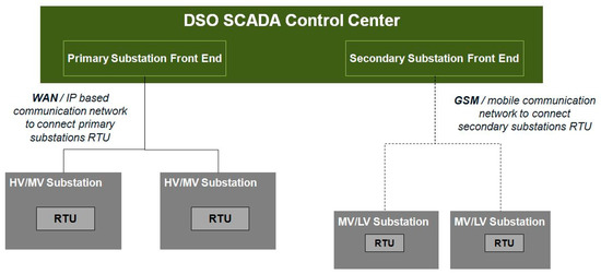
Figure 1.
State of the art of the Supervisory Control And Data Acquisition SCADA in Italy.
The architecture is not appropriate to sustain the new DSO role, as it requires: (a) an enhancing of the capacity for managing new devices and information coming from the network (e.g., power output measurements of DGs, DGs busbar voltage measurements, switches status and transmit DGs’ voltage and power set-points), and (b) new algorithms for the real-time operation of the network. Finally, new dispatching capabilities are also necessary, in order to manage the resources connected to the DN to provide Ancillary Services, and to give them the option to participate in the Ancillary Services Markets in a way consistent with a country’s regulatory framework [52,53]. In particular, the SCADA must provide the following new functionalities:
- Load and Generation Forecast System;
- Network Calculation Algorithm System (NCAS): Network Estimation and control algorithms (Voltage Regulation, Optimal Power Flow, Emergency Restoration, etc.).
To implement them, the following characteristics are required: an IP-based communication network among Primary Substation and the network (based on IEC 61,850 interfaces), an interface for transformer protection and the tap changer, and an interface for the DN devices. Further, more Secondary Substation measurements (real and reactive powers from feeders and transformers, and busbar voltage measurements) and advanced automation procedures (fault detection, local regulation) are necessary. Finally, on the Customers Side of the Secondary Substation, some new devices must be provided to collect user substation measurements, and to control user plants according to set-points calculated by NCAS. This architecture is illustrated in Figure 2.
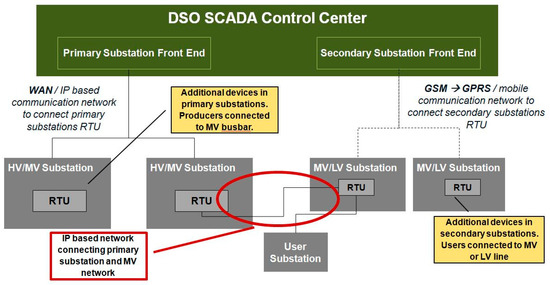
Figure 2.
Evolved Smart Distribution System Operator’s (DSO) SCADA.
3. Voltage Control Approaches
3.1. Local Control Strategy
Nowadays, Grid Codes already rule the direct contribution of DG units to voltage control at the PCC. In [26], with respect to the Italian scenario, authors have already investigated the possible solutions proposed by the national grid code and pointed out the achievable performances. In all the proposed control laws, a DG unit is going to contribute to the voltage control simply by evaluating the real-time voltage phase at the PCC; eventually, maximum/minimum thresholds are imposed to the control law, in order to preserve the dynamic stability. Thus, all the methods involve two conditions: a normal operating situation, and a situation where first thresholds are violated. Among all the presented strategies in [26], the volt–var control, illustrated in Figure 3, shows better performances regarding increasing the HC and containing energy losses. Interestingly, papers [54,55] study similar Local Strategies applied in the LV grids of photovoltaic plants [54] and prosumers [55], and similar conclusions are drawn regarding the volt–var control. In normal operation, the measured voltage stays within the first threshold defined by the range (V1; V2), and thus the DG unit operates at the unitary power factor; if the measured voltage is outside the range (V1; V2), then the DG unit’s reactive power will change linearly with the violation of the first thresholds until the maximum value is reached.
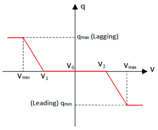
Figure 3.
Best Local Control strategy according to [26].
The main benefit of such an approach consists of a solid improvement of the HC of the grid, in very minor incremental costs, limited to a generator retrofit (in order to fit the grid code’s reactive power requirements), whilst the main drawback consists of the uncoordinated management of the reactive power injections. Moreover, the Local Voltage Control strategy does not need any telecommunication capabilities, allowing for very fast deployment.
Lastly, nowadays a local voltage control strategy is mandatory in the Italian context [17], and ends up as the performance proxy for more advanced options.
3.2. Coordinated Control Strategy
Nowadays, Distribution Networks have a very limited number of sensors, and are managed by standard telecommunication architecture, i.e., a limited amount of data can be shared at a limited speed (PLC and GPRS technologies are the most common ones).
In the new Smart Grid paradigm, the DN is supposed to have a new telecommunication architecture and a large number of sensors spread throughout the grid, which will allow for gathering enough data to perform a grid state estimation and a close to real-time optimization and control of the system. This approach is identified in the literature as a Centralized Voltage Control. Unfortunately, such an evolution is not straightforward, and, in particular, the economic feasibility could be complex to solve.
In order to identify an effective approach for managing DG units, in this paper a novel Coordinated Voltage control architecture is proposed. In particular, the goal is to adapt the assets already in place, in order to coordinate the DG units deployed in the grid and overcome the limits that characterize the local approach. Unlike the CVC approaches available in the literature, the approach proposed here is based on information generally already available in DMS/SCADA, and does not require high computational skills. Indeed, DG units only have to be provided with equipment capable of sampling the voltage phasor and exchanging data with the DSO’s SCADA. In managing such information, the goal is to implement a simple coordination algorithm not based on a complete state estimation procedure (i.e., based just on the samples related to the DG units).
Given a feeder and a DG unit exchanging power with it (Figure 4), the voltage drop over the line can be easily calculated as a function of the DG’s generated power and line impedance. Therefore, denotes the voltage phasor at the PCC; , the voltage phasor at the receiving end of the line (in general terms, the point of connection with the primary HV/MV transformer, therefore, the slack bus); , the complex impedance of the considered line; , the current phasor flowing from the DG unit to the slack bus, and the complex power generated by DG. Accordingly, one can obtain the voltage drop phasor:
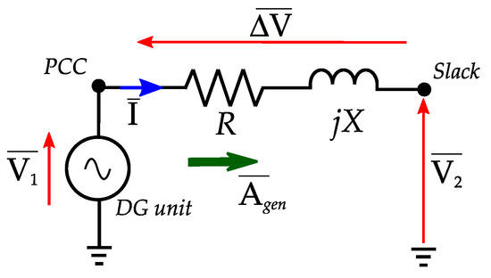
Figure 4.
Electric circuit of a typical distribution line connecting a DG unit.
The goal of Coordinated Control is to limit such a voltage drop in case thresholds are violated. This can be performed by adopting an approximated approach, i.e., calculating the sensitivity of voltage drop with respect to the DG unit’s reactive injection, while considering the real power injection constant. Therefore, in order to decrease the voltage drop for a given network bus, i.e., to fix it at a target value that solves the voltage violations, the following equation can be used:
where is the set of DGs in the DN, while the sensitivity of the voltage drop can be calculated using Equation (4).
In practical terms, in order to change the voltage drop, the proposed procedure starts from the evaluation of the DG unit with the highest sensitivity and, consequently, with the definition of the reactive power set-point required to solve the problem. If the reactive capability of the selected DG unit will be lower than the required reactive injection, a second unit (selected as the one with the second highest sensitivity) will be scheduled, and so on up to involving all the DG units connected in the feeder.
To adopt such an approach, the DSO’s SCADA would be in charge of quantifying the sensitivities of the voltage drop with respect to the DG unit’s reactive injection. This results in topological information, and could be easily calculated by Equation (4). In particular, by adopting the approximated formulation of the voltage drop, i.e., neglecting the imaginary part of Equation (4) (such an approximation is well known and investigated in the literature [56]), the coordinated voltage control law could be approximated as in Equation (6) (where Xk is the line reactance between the PCC of DG unit k and the HV/MV transformer, whilst V1 is the nominal voltage of the feeder).
The flowchart of Figure 5 resumes the main steps of the proposed procedure. First, if during real-time monitoring of the DN a voltage violation is detected (step 0 in Figure 5), the SCADA will calculate the voltage drop target, i.e., , and the voltage drop sensitivities with respect to the DG’s reactive power, i.e., (steps 1 and 2 in Figure 5). Then, a fast iterative process is engaged in order to determine the amount of reactive power necessary to solve the voltage violation, i.e., : first, the DG with maximum sensitivity is selected, and is determined (step 3). If, applying this variation to the current reactive power produced by the DG, i.e., , does not lead to a reactive power limits violation, then the selected generator can fully mitigate the voltage violation, and the process is stopped by applying the new reactive generation level, . If a reactive power limits violation occurs, then is set to the violated limit, and are updated accordingly, while the sensitivity of the currently considered DG is removed from the database (step 4 in Figure 5). At this point, a new iteration is executed by going back to step 3.
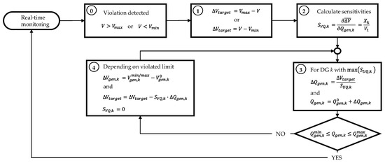
Figure 5.
Coordinated Control strategy flowchart.
3.3. Centralized Control Strategy
This approach requires an accurate real-time knowledge of the DN’s state, as given by a state estimation algorithm, as it consists of a close to real-time optimization and control of the network. Therefore, the approach proposed in this section is formulated as an ORPF problem, especially designed for DNs. Like any optimization problem (OP), the ORPF model consists of an objective function, reflecting the DSO’s goals and subject to various equality and inequality constraints, expressed as mathematical functions.
3.3.1. Objective Function
The typical goal of the ORPF is to minimize the real energy losses in the system. In a classical ORPF, this translates to minimizing the real power produced by the slack generator; as all other generators have their real power production fixed, the demand is also fixed, and, according to the active power balance of the network (7), the slack generator will compensate any change in the active power losses:
where is the sum of the real power produced by all the generating units in the network, is the total real power demand in the network, and are the real power losses in the grid.
In these circumstances, the objective function would be:
where is the real power produced by the slack generator.
In a DN, the slack generator is represented by the HV External Grid connected at the HV side of primary Substation’s busbar. Moreover, unlike in a transmission network, in a DN, the voltage profile no longer mainly depends on the reactive power flow, as the P–V decoupling hypothesis is no longer true given the high R/X ratio. Therefore, it is possible to modify the voltage profile by also changing the real power of all the generators (not only the slack bus). On the other hand, this should be avoided as much as possible, due to economic reasons; for example, renewable plants normally operate at maximum available power, and their redispatch would essentially mean the curtailment of a part of their production capacity. In this context, the objective function can be reformulated as follows:
where is the set of DGs that allow real power control, while the superscript “0” indicates the initial value of the corresponding quantity; the set includes the slack bus, and SL is the set that represents the slack generator.
Considering the power required by the demand constant, according to (7), the first term of (9) holds for real power-loss minimization, while the second term is a penalty term the role of which is to prevent the deviation of the real power output of the generators (except the slack bus) from their scheduled profile. In Equation (9), is a penalty factor fine-tuned such that the real power output of the generators does not deviate from the scheduled value, unless in cases of emergency, when it is strictly necessary (e.g., line contingency, poorly available reactive resources).
3.3.2. Constraints
The constraints to which objective function (9) is subject need to force the optimal solution to a feasible operating point of the network. Thus, generally, these constraints include (i) the nodal power’s balance equations for each bus of the network (the Power Flow equations); (ii) the generators’ capability limits; (iii) the branch maximum currents; and (iv) the nodal voltage limits.
The Power Flow (PF) constraints, modeling the nodal real and reactive power balance at each bus of the network, are:
where and are the total real and reactive powers of the generators connected at bus k, respectively; and are the real and reactive powers absorbed by the demands connected at bus k, respectively; and are the nodal voltage magnitudes of bus k and bus m, respectively; and are the nodal voltage phases of bus k and bus m, respectively; is the magnitude of the kmth element of the bus admittance matrix ; is the phase of the kmth element of the bus admittance matrix , while N is the total number of buses of the network.
The DG’s capability constraints are a complex matter. On the one hand, as was shown in the first section of the paper, there are the regulation-imposed limits and the physical limits of DGs. On the other hand, as one has seen in the previous section, there are DGs that can modify their real power output if needed, and there are those that cannot for various reasons. The latter is easy to model: with the real power fixed, and the DG capability curves or the regulatory framework limits given, the minimum and maximum reactive power limits corresponding to the current’s real power output (or, in general, nominal real power output) can be determined and fixed. In this case, the capability constraints are mathematically expressed using lower–upper bound constraints:
where and are the minimum and maximum reactive power outputs, given by the capability curve at for generator i.
For the DGs with variable real power, the capability curve needs to be modeled in detail. Considering that the majority of DGs are actually RES generators, and that the future evolution of RES technologies is towards full-converter generators (photovoltaic plants and Permanent Magnet Synchronous Generator wind plants), the full-converter limits will be considered here. However, the proposed model can be adapted to other DG types, like conventional synchronous generators.
First, referring to the physical capability limits, the generated real power is limited by its upper and lower bounds, as:
where and are the minimum and maximum real power output of generator j, respectively. In general, corresponds to the initial operating point of the DG, i.e., , as the RES is set to operate at maximum efficiency.
Then, the capability curve of a full converter consists of the maximum current given by its thermal limit. Knowing that the voltages in the network are in general close to the nominal value, the voltage can be considered actually constant, and a simple quadratic constraint can be introduced to model the maximum current limit in terms of power limits:
where is the maximum apparent power of generator k, given by the maximum current limit of the convertor at the nominal operating voltage.
In practice, the reactive power limits are not only imposed by physics, but also by the regulatory framework. According to [49], the DG plants need to guarantee a reactive power band that is either defined by the actual level of real power production, i.e., , through a limit power factor (), is constant (e.g., corresponds to the nominal operating point of the machine), or is a combination of the two. According to [50], analogous constraints can also apply at the TSO–DSO interface, and therefore, to the slack generator. These limits are illustrated in Figure 6.
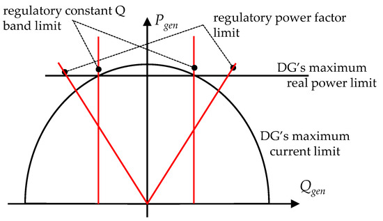
Figure 6.
The Renewable Energy Resources (RES) generator’s physical vs. regulatory capability limits.
Figure 6 shows that the regulatory minimum requirements are tighter than the physical capability of the DG. From the operational point of view, this means that respecting the regulatory framework’s minimum requirements will, in general, stress the DG to a lesser extent. Therefore, there is no motivation for the plant owner to go beyond the regulatory framework requirements, and thus, these limits need to be correctly modeled. While constant band limits can be modeled by extending (11) to all generators, the power factor limit needs to be modeled separately:
where is the limit power factor for both inductive and capacitive operations.
This remains a strict constraint, since generators are not allowed to produce at a power factor lower than the limit one, even if they physically can. Since this limit can be very tight at low levels of real power production (see Figure 6), it may lead to the divergence of the ORPF, due to the lack of reactive resources for keeping the voltage profile within acceptable limits. Therefore, it is necessary to allow the limit power factor constraints to be violated in case of emergency, if the physical capability of the DG allows it [that is, if (12) and (13) are respected]. For this reason, constraint (14) is redefined into an elastic constraint by introducing a slack variable that quantifies the power factor limit violation:
In Equation (15), is the positive slack variable. In order to assure that is minimized, ideally taken to a null value, a penalty factor is introduced in the objective function (9):
In Equation (16), is a penalty factor fine-tuned to assure that the limit power factor is violated only if there are not enough reactive resources to hold the voltage profile within the limits, or, in other words, there is a feasible solution to the ORPF problem (that the effect of must be stronger than that of ).
The implemented limits are depicted in Figure 7. Besides the power factor limits, the capability curves are similar to the ones for a traditional synchronous machine; only the field limits are missing. The latter are difficult to introduce, as they involve the modeling of a synchronous machine using the Behn–Eschemburg method (induced electro-motive force behind synchronous reactance), a model which would further complicate the formulation. However, the field limits of a synchronous machine could be modeled in a simplified way, i.e., either as a rough lower–upper bound approximation—Equation (11)—or as a convex approximation consisting of a linear function of and , as in [47].
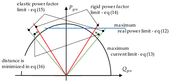
Figure 7.
Modeled capability curved for a RES generator.
Moving further, the branch’s current-constraining role is to prevent the currents flowing through the branches of the network and assuming values higher than the capacity of the branch itself. Due to the presence of power losses and the shunt capacitance of the cable, it is necessary to consider the currents at both ends of a branch. Thus, in a general vector form, these constraints are:
where is the vector of branch current magnitudes at the “from” bus; is the vector of branch current magnitudes at the “to” bus, and is the vector of maximum branch currents.
Either or are determined as the magnitude of the complex branch currents:
where is the vector of nodal voltages phasors, and is the branch admittance matrix.
Equation (17) introduces a high degree of non-linearity, which has a negative impact on the computation time of the ORPF. Thus, to limit this effect, Equation (17) is written only for the branches for which the initial current is above a certain threshold. Setting the threshold at 80% results in the insertion into (17) of all branches that could suffer current violations in the final ORPF solution.
Lower–upper bound constraints for the nodal voltage profile are introduced in vector form:
where and are the vectors of the lower and upper bounds for the nodal voltage magnitude, .
3.3.3. Modeling the OLTC Transformer
The OLTC transformer is one of the most important voltage control devices in DNs, and therefore it cannot be neglected as a resource by a centralized voltage control algorithm. However, its representation inside the ORPF model is not simple; the control variable, i.e., the tap ratio, is a discrete variable, since it is associated with a mechanical tap changer, and its explicit presence in ORPF constraints would lead to a MINLP instead of a NLP. This would render the optimization problem difficult to solve within the fast computation times required by a real-time implementation. A good solution would be to approximate it with a continuous variable, and round it to the nearest feasible discrete value following ORPF convergence. This solution, though, is still uncomfortable, as it involves converting parameter to a variable dependent on the square of the tap ratio (if k = m), or on the tap ratio (if k m). This increases the non-linearity degree of the ORPF model, making some elements of the Hessian of the ORPF less robust and difficult to evaluate, in particular the PF and branch current constraints.
A simpler and more elegant solution can be adopted instead. This solution is possible only due to the characteristics of DNs: they are radial, and only the HV/MV transformers are OLTC transformers. Therefore, the ideal transformer part of the electric transformer model will always be connected at the slack (HV) bus, as shown in Figure 8. Here, the shunt parameters are neglected for simplification, but the proposed solution works also if they are considered.
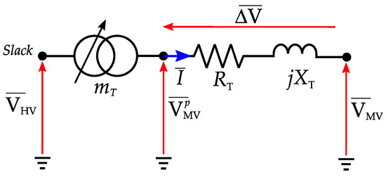
Figure 8.
On-Load Tap Changing (OLTC) Electric transformer in a DN.
First, since the HV bus is also the slack bus, the nodal voltage phasor is characterized by a null phase, and thus, the tap ratio is:
while, according to Figure 8, the nodal voltage phasor at the MV terminals of the transformer is:
In the exact modeling approach, is constant, as it is imposed by the external HV transmission network, while is variable within its technical limits, i.e., . However, the same equivalent effect, i.e., (21), can be obtained if is fixed to a constant value (the nominal value) and is free to vary within
where is the value imposed by the external HV transmission network.
Thus, in ORPF, it is possible to model the tap ratio indirectly, as a continuous variable, by considering the voltage of the slack bus variable [within the range defined by (22)] as a constant instead, with its phase constant and equal to null, while the tap ratio is fixed to the nominal value. In this way, in the optimization model, remains a constant parameter. Following ORPF convergence, it is possible to calculate the value of from (21) using , and round it to the nearest feasible discrete value, to obtain the actual value of .
4. Results and Discussion
4.1. Case Study Description
All previously described algorithms have been implemented in a MATLAB environment [57]. The Local Control algorithm has been emulated in MATLAB using an iterative procedure, where PF calculations are performed sequentially until a convergence criterion is satisfied. Here, for a generic iteration, the reactive output of DGs is determined using the control law characteristic and the nodal voltage magnitude resulting from a previous PF calculation as an equivalent measure. Convergence is found when the reactive power output of all generators varies from one iteration to another within a defined threshold. The procedure is initialized by considering all DGs at unitary power factor. A Coordinated Control algorithm has been implemented using a simpler approach, which applies the following steps: (i) an initial PF calculation reflecting the absence of any control scheme (DGs at unitary power factor) to determine the initial voltage profile, and thus detect any voltage violation; (ii) in case a voltage violation is detected, the calculations shown in Figure 5 are executed in order to find the new power output of the DGs; (iii) a final PF calculation is performed to find the new operating point of the network; in the case where this point also presents violations, the process from (i) is repeated, emulating the real-time feedback loop described in Figure 5. For both Local Control and Coordinated Control, the PF tool consists of an in-house developed Newton–Rhapson algorithm [6]. Finally, the Centralized Control algorithm has been implemented as an in-house interior-point method algorithm, which finds the optimal solution of the ORPF described in Section 3.3.
All implemented algorithms have been tested on a realistic DN feeder, of which the data has been adapted from an actual DN used in one of the smart grid pilot projects shown in [6]; specifically, a feeder characterized by a large penetration of photovoltaic generation. The test DN, the graph of which is shown in Figure 9, consists of 101 nodes and 35 DGs, of which 28 are photovoltaic plants, while the rest are conventional generators. The graph of Figure 9 has been obtained using only branch connectivity, without any correlation to the actual geographical data. The analyzed feeder is characterized by a total installed photovoltaic generation of 7.3 MW, and a maximum installed load of 4.5 MW, while the cable directly connected to the HV/MV transformer has a capacity of 5.5 MVA.
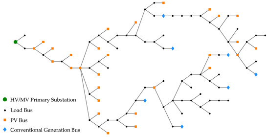
Figure 9.
Studied distribution feeder.
In order to evaluate the performances of the three voltage control strategies, a typical summer day has been considered, and demand/generation power profiles have been defined for every 15 min of the considered day. Overall, the profiles of 96 points have been obtained, and they are shown in Figure 10. From the reactive power point of view, the demand is characterized by an average lagging power factor of 0.94, and the photovoltaic generation reactive limits are set at limit power factor 0.9, meaning the available reactive capability diminishes with generated real power, while the conventional generators’ reactive limits have been calculated based on the capability limits of the corresponding synchronous machines at the current level of real power production.
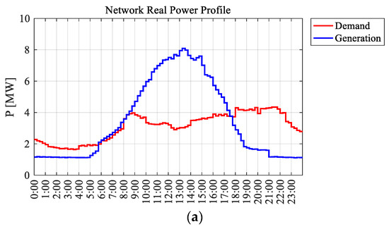
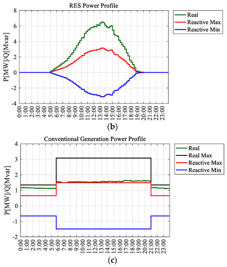
Figure 10.
Adopted generation/demand profiles for the studied distribution feeder: (a) overall generation and demand real power profile; (b) RES power profile; (c) conventional generation power profile.
Figure 11 shows the voltage and branch loadability profiles obtained in the absence of any voltage control strategy, i.e., with DGs operating at unitary power factor and nominal OLTC. No current violations occur, but the voltage profile violates the maximum limit in the first period of the photovoltaic generation’s increase, i.e., when the generation and demand are almost balanced, and the capacitive effect of the cables is therefore emphasized and in the peak period of photovoltaic generation (i.e., when the power flow is reversed, and the voltage drop is thus directed from the DGs to the primary Substation). The minimum voltage limit is violated at early night hours, when generation is at its lowest levels and demand is very high. Clearly, a voltage control strategy is needed.
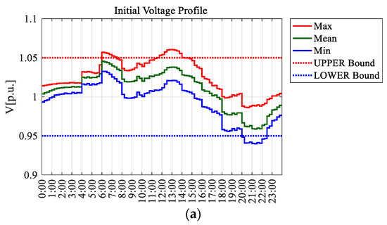
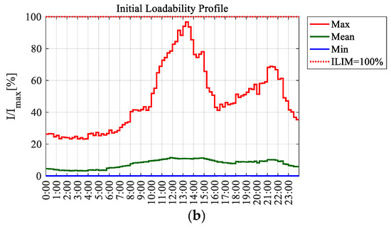
Figure 11.
Initial results: (a) voltage and (b) loadability profiles.
Figure 12 shows the real power loss profiles obtained without applying any voltage control strategy. The power losses increase with the magnitude of the currents, but are also influenced by the voltage profile (higher voltages = lower losses). Overall, the real energy losses during the entire day are ≅2.81 MWh, which is about 3.38% of the total energy produced by DGs (≅83 MWh).
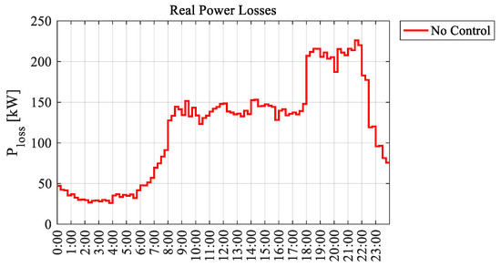
Figure 12.
Initial results: real power losses profile.
4.2. Local vs. Coordinated Control
In this paper, the volt–var law is selected as the Local Control strategy to test, since, as shown in Section 3.2 it is the most efficient Local Control strategy. Figure 13 shows the three adopted configurations for the Local Control strategy. The first threshold [V1; V2] was set to with respect to the nominal voltage of the node, while the limit thresholds (Vmin and Vmax) in Figure 3 (i.e., the voltage values for which the reactive capability limit of the DG is reached) were set up according to the network’s nodal voltage limits in three configurations: C1—where the thresholds are relaxed, with respect to the network’s nodal voltage limits, by , to obtain a relaxed reactive power response; C2—where the thresholds are set up at the network’s nodal voltage limits to obtain a reactive power response matching the network’s nodal voltage limits; and C3—where the thresholds are tightened, with respect to the network’s nodal voltage limits, by , to obtain a stiff reactive power response.
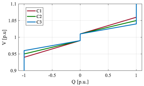
Figure 13.
Local control: volt–var law set-up for simulations.
Figure 14 shows the resulting voltage profiles (Figure 10a,b) and the reactive power responses of the DGs (Figure 10c) for the considered day. First, it can be noticed that Local Control exploits the reactive power resources at any point in time during the day, and in a uniform manner, always providing a response proportional to the deviation of the voltage profile from the nominal value, while the Coordinated Control provides a punctual intervention only in the case of voltage violations—see Figure 14c. For this reason, the voltage profile of Coordinated Control is much closer to the initial profile than the one given by Local Control. Second, Figure 14a,b show that when a large reactive power capability is available (daylight hours—see Figure 10), both control methods can mitigate voltage violations; however, when the available reactive power capability is low (from 21:00 onwards), the Local Control strategy cannot solve the minimum voltage violation even in its stiff setup (C3), while the Coordinated strategy always can. This is an expected result, since the Local strategy cannot explicitly solve voltage violations (it can implicitly), while Coordinated Control is explicitly designed for this purpose. This means that Local Control law parameters need to be carefully set-up over a wide range of possible operating conditions.
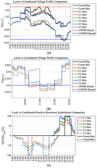
Figure 14.
Local vs. Coordinated Control results: (a) DN’s voltage profile; (b) DN’s voltage profile—detail of night hours; (c) DGs reactive power response with respect to available capability.
Figure 15 shows the resulting loadability profiles for the considered day. Except for the peak photovoltaic production hours, detailed in Figure 15b, the currents in the DN are well within the limits. However, during the peak photovoltaic production hours, the currents in some branches of the network violate the limit. Comparing the two strategies, it is evident that Local Control is more prone to activate current violations, even in its most conservative set-up, i.e., C1. Clearly, current violations result from the contribution of DG’s reactive power to the line currents that, initially (i.e., when DGs operate at null reactive power output), are close to the limits, but do not violate them (see Figure 11). The impact of Local Control is much stronger as, by design, this strategy activates the reactive power generation of many DGs, while Coordinated Control only uses the reactive power of a few. This is an important observation, since these algorithms are designed to operate in poorly observable DNs, where most of the branch currents are not measured.
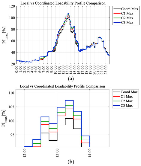
Figure 15.
Local vs. Coordinated Control results: (a) DN’s loadability profile; (b) DN’s loadability profile (detail on photovoltaic peak hours).
Finally, Figure 16 shows the real power loss variations, with respect to the initial scenario. Both the Local and the Coordinated strategy lead to an increase of power losses in the DN, but the Coordinated strategy has a minor impact. This can be explained in light of the previous results: the Coordinated strategy is less intrusive (it activates fewer times, and it involves less DGs), while both strategies need to take actions that lead to the increase of real power losses, as in many cases the voltage profile is lowered to solve or prevent maximum voltage violations.
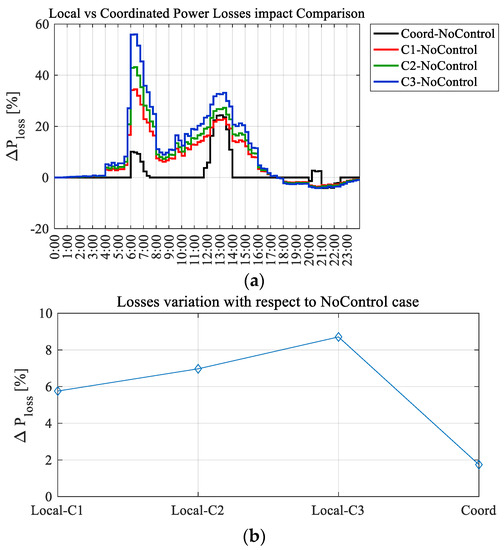
Figure 16.
Local vs. Coordinated Control real power losses: (a) profile; (b) aggregated.
Synthesizing the results, we see that Coordinated Control is the more robust approach. However, if the DN’s control and supervision architecture does not allow the implementation of the Coordinated scheme, the Local strategy is the only possible solution (which is also imposed by the regulatory framework). If this is the case, the results show that Local Control requires a careful tuning of its defining parameters, as it is prone to produce violations under peculiar operating conditions of the DN. The authors studied various optimal tuning solutions for Local Control laws in [15,56]; these approaches are promising, but in the absence of proper network monitoring, they depend heavily on the statistical estimation of generation/demand profiles, which may not ensure a strong correlation with the actual operating conditions of the grid. On the other hand, if the DN’s control and supervision architecture allows the implementation of Coordinated Control, then Local Control could either be abandoned or, in correspondence with the regulatory framework, could work in tandem with Local Control; the base operation could be provided by Local Control (with a less stiff set-up), which, in spite of the disadvantages, tries to keep the voltage profile close to nominal, while the Coordinated Control would override the Local Control in cases of detected violations.
4.3. Centralized Control
The ORPF model has been set-up to (i) control both the OLTC of the HV/MV transformers from the primary Substations, and the DG unit’s output power (Configuration 1), or (ii) control only the DG units, as in the case of the other two control strategies (Configuration 2). Figure 17 shows the main computation steps needed in both cases. Configuration 1 involves three steps: an ORPF calculation at a continuously variable tap, followed by an intermediate step where the actual value of the tap is obtained by rounding it to the nearest feasible discrete value. These steps are detailed in Section 3.3.3, while the last step involves a new ORPF computation at a fixed tap in order to mitigate the negative impact of rounding; this final step is carried out at a fixed slack voltage magnitude, i.e., at the value given by the measurements. Configuration 2 involves running a single ORPF calculation at a fixed tap, i.e., at the nominal tap; therefore, in this case as well, the slack voltage magnitude is fixed at the value given by the measurements.
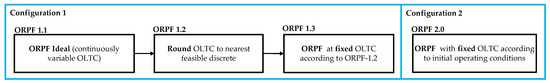
Figure 17.
Tested Optimal Reactive Power Flow (ORPF) configurations.
Additionally, the simulations have been performed in four variants, obtained by setting the maximum allowed loadability to various levels: variant a, where the maximum loadability is fixed at 100% of the thermal limits of the lines, that is, according to network data, and variants b, c and d, where the maximum loadability is fixed at 95%, 90% and 85% of the thermal limits of the lines, respectively. Mathematically, these variants will numerically stress the ORPF; practically, forcing the current limits to values lower than the actual limits provides a margin to protect the network against current violations resulting from unexpected variations of the DG’s output or demanded power.
Last but not least, the photovoltaic generators are modeled inside the ORPF as DG units with curtailable real power, while the conventional generators are modeled as uncurtailable DG units. In detail, the capability limits of the photovoltaic plants are modeled by Equations (12), (13) and (15), with , while the capability limits of the conventional plants are modeled by Equation (11). Therefore, with respect to the initial situation shown in Figure 10 and detailed in Section 4.1, the ORPF can decrease, in case of emergency, the real power produced by the photovoltaic plants, while also losing the reactive power margin due to the limit power factor. As discussed in Section 3.2., if this reduction in reactive power margins makes it impossible for the ORPF to find a feasible operating point, then the elastic constraints (15) need to allow the relaxation of this limit. For this reason, following a series of preliminary tests, the penalty coefficients and of objective function (16) were set up to 100 and 300, respectively.
Figure 18 shows the results related to the ORPF constraints for the first step of Configuration 1 in variant a, i.e., ORPF 1.1.a. This case is considered the ideal and reference case, as the tap ratio is a continuous variable (ideal case), and the current limits are set to the actual network limits, not artificially forced. For all considered time windows, the voltage profile is pushed against its maximum bounds, while in most situations, to achieve this the reactive resources are also pushed against their maximum limits. This result is normal, as in a power system the real power losses decrease with the increase of the nodal voltage magnitudes. Finally, Figure 18c,d shows that ORPF avoids current limit violations without curtailing any real power generation. Overall, ORPF guarantees the satisfaction of all operational limits, while pushing the operating point of the network against the limits that oppose the minimization of real power losses.
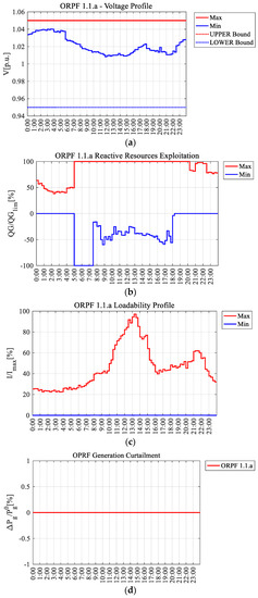
Figure 18.
ORPF 1.1.a results: (a) voltage profile; (b) reactive power response with respect to available capability; (c) DN’s loadability profile; (d) DG’s real power curtailment.
Figure 19 shows the variation of the real power losses for ORPF 1.1.a in all the considered time windows, with respect to the initial (no control strategy) case. In general, a strong reduction of the losses is obtained. Exceptions arise for the time windows where the maximum voltage limit was initially violated and the ORPF had to reduce the voltage in order to mitigate the violation, i.e., from 6:00 to 7:00 and from 12:00 to 14:00 (see Figure 11). However, for these cases, the variations of the power loss with respect to the initial case are well contained, which shows that the designed ORPF can optimally manage the reactive resources even when the network constraints do not allow the real power losses’ minimization. This conclusion is strengthened by comparing Figure 19 with Figure 16a in the hours when maximum voltage is initially violated: all control strategies solve the violation, but only ORPF can contain the increase of real power losses in the network. Finally, the overall real power losses are reduced by ORPF 1.1.a by 7.8%, with respect to the initial operation.
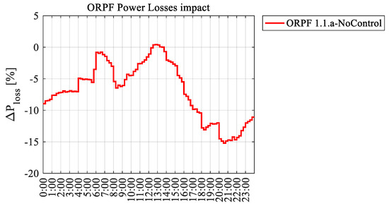
Figure 19.
ORPF 1.1.a relative power losses.
The detailed analysis of ORPF 1.1.a previously performed shows that the ORPF algorithm works properly. Further, for illustrative purposes and exposure containment, some particular aspects will be considered when analyzing the remaining ORPF set-ups. Figure 20, Figure 21 and Figure 22 show the peculiarities of ORPF 1.1 for all considered variants. Figure 20 shows the results related to the loadability of the network’s branches. Figure 20a reports identical results between variants, as long as none of the considered current limits are violated. This happens at peak photovoltaic production hours, detailed in Figure 20b, when the ORPF brings the currents to the violated limits. In conclusion, Figure 20 shows that the ORPF stays as close as possible to the ideal solution of ORPF 1.1.a. Figure 21 shows that the mitigation of the current limits is performed with minimum curtailment action: they occur only for stringent current limits (90% and 85%, respectively), are well contained, and increase with the decrease of the limits. Here, the elastic constraint (15) is never activated, and therefore the current constraints are solved without relaxing the limit power factor.
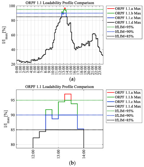
Figure 20.
ORPF 1.1 loadability profile results: (a) full profile; (b) detail on photovoltaic peak hours.
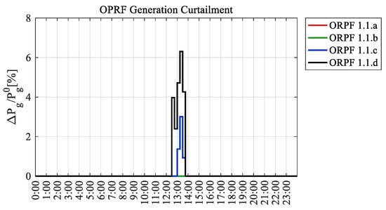
Figure 21.
ORPF 1.1 results: DG’s real power curtailment.
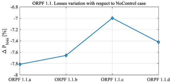
Figure 22.
ORPF 1.1 results: power losses variation with respect to initial case.
Lastly, Figure 22 shows the power loss variation, with respect to the initial conditions, over the entire analyzed period. Generally, in all variants, the power losses are lower with respect to the initial conditions, but they tend to increase with the decrease of the current limit. This is an expected behavior, as tightening the limit reached by the optimal solution worsens the optimal solution. However, ORPF 1.1.d is the exception, since the power losses decrease with respect to ORPF 1.1.c: this can be explained by the fact that ORPF 1.1.d sees a strong curtailment of DGs generation (see Figure 21), which leads to a stronger overall decrease of the currents in the network, and hence, to real power loss reduction.
Figure 23 shows the comparison between ORPF 2 and ORPF 1.1 for all the considered variants, in terms of overall real power losses variation with respect to the initial conditions. Clearly, not considering the OLTC among the variables of the optimization problem drastically limits the performance of the ORPF, as the power losses obtained with the variable OLTC (ORPF 1.1) are reduced about fourfold with respect to the ones obtained with a constant OLTC (ORPF 2). Anyway, even ORPF 2 reduces the power losses with respect to the initial case.
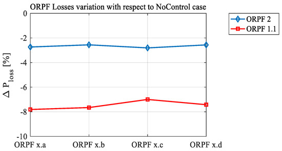
Figure 23.
ORPF 1.1 and ORPF 2 relative power losses with respect to the initial case.
Figure 24 shows the impact on the real power losses of OLTC rounding (ORPF 1.2), and the improving action of the second ORPF run with a constant OLTC (ORPF 1.3). The results are shown in terms of the overall real power variations of ORPF 1.2 and ORPF 1.3, with respect to ORPF 1.1. Clearly, there is a slightly negative impact of rounding the OLTC (about 1% power loss increase with respect to the ideal ORPF results) that can be marginally mitigated by running ORPF 1.3.
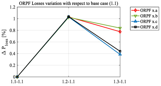
Figure 24.
ORPF 1.2 and ORPF 1.3 power losses with respect to ORPF 1.1.
The results show that Configuration 1 is the “go to” option for DMS implementation, as it offers the best results of the two configurations. However, a real-time application of the ORPF would be feasible only if the computation times were well contained, with respect to the time window for which the ORPF would be employed. Figure 25 depicts the histogram of computation times required for the execution of Configuration 1 over all considered situations (all variations and all time windows, resulting in 384 double executions of the ORPF algorithm—see Figure 17). In most of the cases, computation time does not exceed 2 s, while the maximum registered value is 5.6 s. This is a very good result, as it suggests that the ORPF algorithm can be applied even for a short time window, e.g., about 1 min, at a limit of 30 s. In real life, the average time window should be larger (i.e., a couple of minutes), in order to avoid DN instability due to a too-frequent change of the operating points of the DG units, and in order to cope with the time dynamics of the data acquisition and processing systems. Therefore, the obtained computation time shows the ORPF algorithm can be implemented without any particular issues in a real life DMS.
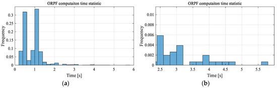
Figure 25.
ORPF computation times statistics: (a) complete histogram; (b) detail of histogram.
Lastly, Figure 26 shows the number of times the OLTC was changed during the analyzed day by ORPF, executed in Configuration 1, for all variants. Averagely, the number of OLTC changes in a single day was 20 out of 96 considered time windows; hence, the OLTC changed at a rate of about 21% during the analyzed day, which is a well contained value (about 1 time per hour).
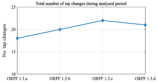
Figure 26.
ORPF Configuration 1 tap changes during analyzed period.
4.4. Results Review and Discussion
Clearly, the two proposed voltage control algorithms in this paper, i.e., the Coordinated Control and the Centralized Control, are suited to two different situations. Coordinated Control is for DNs with a SCADA system reduced to the acquisition of a few measurements across the DN (voltage measurements at DG buses and at key demand buses, real and reactive power outputs of DGs), and with the possibility of tele-controlling the DGs. Centralized Control is for DNs with an evolved SCADA that allows the calculation of the state of the DN through a state-estimation algorithm. Both algorithms have been tested on a realistic DN, but they are not directly comparable.
Coordinated Control has been compared with the currently adopted solution at a regulatory level: the best Local Control strategy that the literature review identified. The main point emphasized by the results is that, to mitigate voltage violations, Local Control tends to exploit all the reactive resources available in a uniform manner, while Coordinated Control uses a few of them extensively. The results showed that this is key in differentiating the performance of the two approaches in favor of Coordinated Control, for which (i) the real power loss variation is better managed; (ii) voltage profile violations are always solved, even when the resources are low; (iii) there is a better chance of avoiding current limit violations (this is important, as with the assumed SCADA system most currents in the network are not measured).
With respect to other CVC approaches present in the literature and thoroughly analyzed in the Introduction section, the proposed Coordinated Control has the advantage of being easily implementable in the majority of state-of-the-art DNs. Indeed, the investigated CVC approaches from the literature were either suitable for small DNs (therefore, microgrids), or they were specialized optimization approaches that, when implemented in a large real DN, required a level of development of the SCADA suited to a Centralized algorithm. However, the proposed Coordinated Control can be easily integrated in a large grid as, nowadays, many DNs are already Local Control-ready, which means that the local measurement of DGs’ plant voltages and powers is already possible; they just need to be properly integrated in the SCADA.
The specifications of the Centralized Control strategy proposed in this paper have been drawn following a thorough literature analysis (see the Introduction section), where the main drawbacks of the state-of-the-art approaches have been revealed. Centralized Control has been designed to mitigate these drawbacks. The numerical tests were not only aimed at emphasizing the raw performance of the algorithm (the minimization of the active power losses), but also at testing the validity of the adopted solutions. These tests were successful since (i) the resulting computation times were well contained, so the algorithm design choices will not cause numerical problems and the proposed strategy can be implemented in real DNs; (ii) the proposed OLTC model worked correctly, and the results showed major improvements in the performance of the algorithm when the OLTC control was used, showing the importance of OLTC representation in ORPF models for DNs; (iii) minimal active power curtailment actions were performed to solve branch congestions when strictly necessary; (iv) the interaction between the regulatory and physical capabilities of the DGs worked flawlessly. Moreover, the results clearly show that Centralized Control works properly from the point of view of its intended goal: the real power losses in the network are significantly reduced with respect to the initial conditions, while the constraints that act against the objective function’s minimization are reached. This means the real power losses are minimized, and the Centralized Control strategy is an ORPF.
5. Conclusions
Firstly, this paper thoroughly investigated the voltage control strategies available in the literature for distribution networks in the presence of Distributed Generators. The strategies have been classified based on the state of development of the SCADA system, from rudimentary to complex. The main characteristics and the flaws of these strategies have been emphasized, relying on the available literature. Secondly, the paper proposed innovative Coordinated and Centralized Control strategies, which are the last two levels of the emphasized classification. Following the bibliographic analysis, the design of these two strategies was performed such that they mitigated the encountered flaws.
A Coordinated Control strategy was designed as a simple and robust algorithm, based on the sensitivity of the voltage profile with respect to the nodal reactive power injection; this algorithm reduced telecommunication, supervision and control requirements, and therefore, is implementable in contemporary large distribution networks. The Centralized Control strategy was designed as a deterministic optimization algorithm, that relies on the particularities of the distribution network and mitigates the most encountered issues within these algorithms, i.e., the discrete On-Load Tap Changer and capability curve modelling. This algorithm requires an advanced telecommunication, supervision and control system for the DN, a system that allows the calculation of the actual state of the grid and its full control.
The designed algorithms have been tested against the Local Control strategy for a realistic distribution network feeder during a typical operating day. The behavior and the advantages of the two algorithms have been discussed. Both offer a better alternative with respect to the current regulatory specifications, and both are implementable in a real distribution network, but their implementation depends on the level of development of the telecommunication, supervision and control system of the DN. The Centralized Control strategy proved the best approach, being the most evolved, but it requires the most out of the telecommunication, supervision and control systems.
Author Contributions
Conceptualization, C.B. and M.M.; Data curation, C.A., R.B. and M.R.; Investigation, V.I.; Methodology, V.I., C.B. and D.F.; Software, V.I., D.F., R.B. and M.R.; Supervision, C.B., M.M. and C.A.; Validation, C.B., M.M., R.B. and M.R.; Writing—original draft, V.I.; Writing—review & editing, V.I., C.B., D.F., M.M. and C.A. All the authors have contributed in the article. All authors have read and agreed to the published version of the manuscript.
Funding
This research received no external funding.
Conflicts of Interest
The authors declare no conflict of interest
Abbreviations
The following abbreviations are used in this manuscript:
| CVC | Coordinated Voltage Control |
| DG | Distributed Generators |
| DN | Distribution Network |
| DSO | Distribution System Operator |
| GA | Genetic Algorithm |
| GPRS | General Packet Radio Service |
| HC | Hosting Capacity |
| HV | High Voltage |
| LV | Low Voltage |
| MINLP | Mixed-Integer Non-Linear Programing |
| MV | Medium Voltage |
| NCAS | Network Calculation Algorithm System |
| NLP | Non-Linear Programing |
| OLTC | On-Load Tap Changer |
| OP | Optimization Problem |
| ORPF | Optimal Reactive Power Flow |
| PCC | Point of Common Coupling |
| PLC | Power-Line Communication |
| PF | Power Flow |
| PSO | Particle Swarm Optimization |
| RES | Renewable Energy Sources |
| SCADA | Supervisory Control And Data Acquisition |
| STATCOM | STATic COMpensator |
| SVC | Static Var Compensator |
| TSO | Transmission System Operator |
References
- Lopes, J.P.; Hatziargyriou, N.; Mutale, J.; Djapic, P.; Jenkins, N. Integrating distributed generation into electric power systems: A review of drivers, challenges and opportunities. Electr. Power Syst. Res. 2007, 77, 1189–1203. [Google Scholar] [CrossRef]
- Directive (EU) 2018/2001 of the European Parliament and of the Council of 11 December 2018 on the Promotion of the Use of Energy from Renewable Sources. Available online: https://eur-lex.europa.eu/ (accessed on 23 April 2020).
- Gallanti, M.; Merlo, M.; Moneta, D.; Mora, P.; Monfredini, G.; Olivieri, V. MV network with Dispersed Generation: Voltage regulation based on local controllers. In Proceedings of the 21th International Conference on electricity Distribution CIRED, Frankfurt, Germany, 6–9 June 2011. [Google Scholar]
- Arrigoni, C.; Bigolini, M.; Bovo, C.; Ilea, V.; Merlo, M.; Monfredini, G.; Subasic, M.; Bonera, R. Smart distribution system the InGrid project and the evolution of supervision & control systems for Smart Distribution System management. In Proceedings of the 2013 AEIT Annual Conference: Innovation and Scientific and Technical Culture for Development, AEIT 2013, Mondello, Italy, 3–5 October 2013. [Google Scholar]
- Berizzi, A.; Bovo, C.; Falabretti, D.; Ilea, V.; Merlo, M.; Monfredini, G.; Subasic, M.; Bigoloni, M.; Rochira, I.; Bonera, R. Architecture and functionalities of a smart Distribution Management System. In Proceedings of the 16th International Conference on Harmonics and Quality of Power, ICHQP 2014, Bucharest, Romania, 25–28 May 2014. [Google Scholar]
- Arrigoni, C.; Bigoloni, M.; Rochira, I.; Bovo, C.; Merlo, M.; Ilea, V.; Bonera, R. Smart Distribution Management System: Evolution of MV grids supervision & control systems. In Proceedings of the 2016 AEIT International Annual Conference, AEIT 2016, Capri, Italy, 5–7 October 2016. [Google Scholar]
- Delfanti, M.; Fasciolo, E.; Olivieri, V.; Pozzi, M. A2A project: A practical implementation of smart grids in the urban area of Milan. Electr. Power Syst. Res. 2015, 120, 2–19. [Google Scholar] [CrossRef]
- Bosisio, A.; Berizzi, A.; Morotti, A.; Pegoiani, A.; Greco, B.; Iannarelli, G. IEC 61850-based smart automation system logic to improve reliability indices in distribution networks. In Proceedings of the 2019 AEIT International Annual Conference, AEIT 2019, Firenze, Italy, 18–20 September 2019. [Google Scholar]
- Coppo, M.; Pelacchi, P.; Pilo, F.; Pisano, G.; Soma, G.G.; Turri, R. The Italian smart grid pilot projects: Selection and assessment of the test beds for the regulation of smart electricity distribution. Electr. Power Syst. Res. 2015, 120, 136–149. [Google Scholar] [CrossRef]
- Bovo, C.; Ilea, V.; Subasic, M.; Rochira, I.; Arrigoni, C. Innovative methodology for observability improvement of distribution networks. In Proceedings of the 2015 IEEE Eindhoven PowerTech, PowerTech 2015, Eindhoven, The Netherlands, 29 June–2 July 2015. [Google Scholar]
- Bovo, C.; Ilea, V.; Subasic, M.; Zanellini, F.; Arigoni, C.; Bonera, R. Improvement of observability in poorly measured distribution networks. In Proceedings of the 2014 Power Systems Computation Conference, PSCC 2014, Wroclaw, Poland, 18–22 August 2014. [Google Scholar]
- Falabretti, D.; Delfanti, M.; Merlo, M. Distribution networks’ observability: A novel approach and its experimental test. Sustain. Energy Grids Netw. 2018, 13, 56–65. [Google Scholar] [CrossRef]
- Singh, R.; Pal, B.C.; Vinter, R.B. Measurement placement in distribution system state estimation. IEEE Trans. Power Syst. 2009, 24, 668–675. [Google Scholar] [CrossRef]
- Bovo, C.; Ilea, V.; Subasic, M. Optimization of Measurement Equipment Placement in Distribution Networks by Genetic Algorithms. In Proceedings of the 2018 IEEE International Conference on Environment and Electrical Engineering and 2018 IEEE Industrial and Commercial Power Systems Europe, EEEIC/I&CPS Europe 2018, Palermo, Italy, 12–15 June 2018. [Google Scholar]
- Yao, Y.; Liu, X.; Li, Z. Robust Measurement Placement for Distribution System State Estimation. IEEE Trans. Sustain. Energy 2019, 10, 364–374. [Google Scholar] [CrossRef]
- Mirbagheri, S.M.; Falabretti, D.; Merlo, M. Voltage Control in Active Distribution Grids: A Review and a New Set-Up Procedure for Local Control Laws. In Proceedings of the 2018 International Symposium on Power Electronics, Electrical Drives, Automation and Motion (SPEEDAM), Amalfi, Italy, 20–22 June 2018. [Google Scholar]
- Italian Electrical Committee (CEI). Reference Technical Rules for the Connection of Active and Passive Users to the LV Electrical Utilities, Technical Standard CEI 0-21, in Italian; CEI: Milan, Italy, 2012. [Google Scholar]
- Vovos, P.N.; Kiprakis, A.E.; Wallace, A.R.; Harrison, G.P. Centralized and distributed voltage control: Impact on distributed generation penetration. IEEE Trans. Power Syst. 2007, 22, 476–483. [Google Scholar] [CrossRef]
- Turitsyn, K.; Sulc, P.; Backhaus, S.; Chertkov, M. Local Control of Reactive Power by Distributed Photovoltaic Generators. In Proceedings of the 2010 First IEEE International Conference on Smart Grid Communications, Gaithersburg, MD, USA, 4–6 October 2010; pp. 79–84. [Google Scholar] [CrossRef]
- Elnashar, M.; Kazerani, M.; Shatshat, R.E.; Salama, M.M.A. Comparative evaluation of reactive power compensation methods for a stand-alone wind energy conversion system. In Proceedings of the 2008 IEEE Power Electronics Specialists Conference, Rhodes, Greece, 15–19 June 2008; pp. 4539–4544. [Google Scholar] [CrossRef]
- Aggarwal, M.; Gupta, S.K.; Madhusudan, M.; Kasal, G. DSTATCOM Control in Low Voltage Distribution System with Distributed Generation. In Proceedings of the 2010 3rd International Conference on Emerging Trends in Engineering and Technology, Goa, India, 19–21 November 2010; pp. 426–429. [Google Scholar] [CrossRef]
- Caples, D.; Boljevic, S.; Conlon, M.F. Impact of distributed generation on voltage profile in 38 kV distribution system. In Proceedings of the 2011 8th International Conference on the European Energy Market (EEM), Zagreb, Croatia, 25–27 May 2011; pp. 532–536. [Google Scholar] [CrossRef]
- Sansawatt, T.; Ochoa, L.F.; Harrison, G.P. Integrating distributed generation using decentralised voltage regulation. In Proceedings of the 2010 IEEE Power and Energy Society General Meeting, Providence, RI, USA, 25–29 July 2010; pp. 1–6. [Google Scholar] [CrossRef]
- Freitas, W.; Vieira, J.C.; Morelato, A.; Xu, W. Influence of excitation system control modes on the allowable penetration level of distributed synchronous generators. IEEE Trans. Energy Convers. 2005, 20, 474–480. [Google Scholar] [CrossRef]
- Ranamuka, D.; Agalgaonkar, A.P.; Muttaqi, K.M. Examining the interactions between DG units and voltage regulating devices for effective voltage control in distribution systems. IEEE Trans. Ind. Appl. 2017, 53, 1485–1496. [Google Scholar] [CrossRef]
- Delfanti, M.; Merlo, M.; Monfredini, G. Voltage Control on LV Distribution Network: Local Regulation Strategies for DG Exploitation. Res. J. Appl. Sci. Eng. Technol. 2014, 7, 4891–4905. [Google Scholar] [CrossRef]
- Marggraf, O. U-Control–analysis of distributed and automated voltage control in current and future distribution grids. In Proceedings of the International ETG Congress, Bonn, Germany, 28–29 November 2017; pp. 1–6. [Google Scholar]
- Hea, C. Advanced local voltage control through polynomial P-Var functions. In Proceedings of the 2019 IEEE Milan PowerTech, Milano, Italy, 23–27 June 2019; pp. 1–6. [Google Scholar]
- Hird, C.M.; Leite, H.; Jenkins, N.; Li, H. Network voltage controller for distributed generation. IEE Proc. Gener. Transm. Distrib. 2004, 151, 150–156. [Google Scholar] [CrossRef]
- Alobeidli, K.A.; Syed, M.H.; El Moursi, M.S.; Zeineldin, H.H. Novel coordinated voltage control for hybrid micro-grid with islanding capability. IEEE Trans. Smart Grid 2015, 6, 1116–1127. [Google Scholar] [CrossRef]
- Bignucolo, F.; Caldon, R.; Prandoni, V. Radial MV networks voltage regulation with distribution management system coordinated controller. Electr. Power Syst. Res. 2008, 78, 634–645. [Google Scholar] [CrossRef]
- Zhou, Q.; Bialek, J.W. Generation curtailment to manage voltage constraints in distribution networks. IET Gener. Transm. Distrib. 2007, 1, 492–498. [Google Scholar] [CrossRef]
- Senjyu, T.; Miyazato, Y.; Yona, A.; Urasaki, N.; Funabashi, T. Optimal distribution voltage control and coordination with distributed generation. IEEE Trans. Power Del. 2008, 23, 1236–1242. [Google Scholar] [CrossRef]
- Nimpitiwan, N.; Chaiyabut, C. Centralized control of system voltage/reactive power using genetic algorithm. In Proceedings of the 2007 International Conference on Intelligent Systems Applications to Power Systems, Niigata, Japan, 5–8 November 2007; pp. 1–6. [Google Scholar] [CrossRef]
- Madureira, A.G.; Pecas Lopes, J.A. Coordinated voltage support in distribution networks with distributed generation and microgrids. IET Renew. Power Gener. 2009, 3, 439–454. [Google Scholar] [CrossRef]
- Mehmood, K.; Khan, S.; Lee, S.; Haider, Z.M.; Rafique, M.K.; Kim, C. A real-time optimal coordination scheme for the voltage regulation of a distribution network including an OLTC, capacitor banks, and multiple distributed energy resources. Int. J. Electr. Power Energy Syst. 2018, 94, 1–14. [Google Scholar] [CrossRef]
- Baran, M.E.; El-Markabi, I.M. A multiagent-based dispatching scheme for distributed generators for voltage support on distribution feeders. IEEE Trans. Power Syst. 2007, 22, 52–59. [Google Scholar] [CrossRef]
- Farag, H.E.Z.; El-Saadany, E.F.; Seethapathy, R. A two ways communication-based distributed control for voltage regulation in smart distribution feeders. IEEE Trans. Smart Grid 2012, 3, 271–281. [Google Scholar] [CrossRef]
- Kulmala, A.; Repo, S.; Jarventausta, P. Coordinated voltage control in distribution networks including several distributed energy resources. IEEE Trans. Smart Grid 2014, 5, 2010–2020. [Google Scholar] [CrossRef]
- Ranamuka, D.; Agalgaonkar, A.P.; Muttaqi, K.M. Online coordinated voltage control in distribution systems subjected to structural changes and DG availability. IEEE Trans. Smart Grid 2016, 7, 580–591. [Google Scholar] [CrossRef]
- Angioni, A.; Sadu, A.; Ponci, F.; Monti, A.; Patel, D.; Williams, F.; della Giustina, D.; Dedè, A. Coordinated voltage control in distribution grids with LTE based communication infrastructure. In Proceedings of the 2015 IEEE 15th International Conference on Environment and Electrical Engineering (EEEIC), Rome, Italy, 10–13 June 2015; pp. 2090–2095. [Google Scholar] [CrossRef]
- Berizzi, A.; Bovo, C.; Merlo, M.; Delfanti, M. A GA approach to compare ORPF objective functions including secondary voltage regulation. Electr. Power Syst. Res. 2012, 84, 187–194. [Google Scholar] [CrossRef]
- Ilea, V.; Bovo, C.; Merlo, M.; Berizzi, A.; Marannino, P. Reactive power flow optimization in power systems with hierarchical voltage control. In Proceedings of the 17th Power Systems Computation Conference, PSCC 2011, Stockholm, Sweden, 22–26 August 2011. [Google Scholar]
- Delfanti, M.; Falabretti, D.; Fiori, M.; Merlo, M. Smart Grid on field application in the Italian framework: The AS SE. M. project. Electr. Power Syst. Res. 2015, 120, 56–69. [Google Scholar] [CrossRef]
- Jakus, D.; Vasilj, J.; Sarajcev, P. Voltage control in MV distribution networks through coordinated control of tap changers and renewable energy sources. In Proceedings of the 2015 IEEE Eindhoven PowerTech, Eindhoven, The Netherlands, 29 June–2 July 2015; pp. 1–6. [Google Scholar] [CrossRef]
- Sheng, W.; Member, S.; Liu, K.; Cheng, S.; Meng, X.; Dai, W. A Trust Region SQP Method for Coordinated Voltage Control. IEEE Trans. Smart Distrib. Grid 2016, 7, 381–391. [Google Scholar] [CrossRef]
- Stock, D.S.; Sala, F.; Berizzi, A.; Hofmann, L. Optimal Control of Wind Farms for Coordinated TSO-DSO Reactive Power Management. Energies 2018, 11, 173. [Google Scholar] [CrossRef]
- Santoso, S.; Saraf, N.; Venayagamoorthy, G.K. Intelligent Techniques for Planning Distributed Generation Systems. In Proceedings of the 2007 IEEE Power Engineering Society General Meeting, Tampa, FL, USA, 29 May 2007; pp. 1–4. [Google Scholar] [CrossRef]
- Ellis, A.; Nelson, R.; Von Engeln, E.; Walling, R. Review of existing reactive power requirements for variable generation. In Proceedings of the 2012 IEEE Power and Energy Society General Meeting, San Diego, CA, USA, 22–26 July 2012; pp. 1–7. [Google Scholar] [CrossRef]
- Stock, D.S.; Venzke, A.; Hennig, T.; Hofmann, L. Model predictive control for reactive power management in transmission connected distribution grids. In Proceedings of the 2016 IEEE PES Asia-Pacific Power andEnergy Engineering Conference (APPEEC), Xi’an, China, 25–28 October 2016; IEEE: Piscataway, NJ, USA, 2016; pp. 419–423. [Google Scholar]
- Berizzi, A.; Bovo, C.; Ilea, V.; Merlo, M.; Monfredini, G.; Subasic, M.; Arrigoni, C.; Zanellini, F.; Corti, F.; Rochira, I. Advanced functions for DSOs control center. In Proceedings of the 2013 IEEE Grenoble Conference PowerTech, POWERTECH 2013, Grenoble, France, 16–20 June 2013. [Google Scholar]
- Migliavacca, G.; Rossi, M.; Six, D.; Džamarija, M.; Horsmanheimo, S.; Madina, C.; Kockar, I.; Morales, J.M. SmartNet: H2020 project analysing TSO–DSO interaction to enable ancillary services provision from distribution networks. CIRED-Open Access Proceed. J. 2017, 1, 1998–2002. [Google Scholar] [CrossRef]
- Gerard, H.; Puente, E.I.R.; Six, D. Coordination between transmission and distribution system operators in the electricity sector: A conceptual framework. Util. Policy 2018, 50, 40–48. [Google Scholar] [CrossRef]
- Schultis, D.-L. Comparison of local volt/var control strategies for PV hosting capacity enhancement of low voltage feeders. Energies 2019, 12, 1560. [Google Scholar] [CrossRef]
- Schultis, D.-L.; Ilo, A.; Schirmer, C. Overall performance evaluation of reactive power control strategies in low voltage grids with high prosumer share. Electr. Power Syst. Res. 2019, 168, 336–349. [Google Scholar] [CrossRef]
- Mirbagheri, S.M.; Merlo, M. Optimal reactive power flow procedure to set up an effective local voltage control. Sustain. Energy Technol. Assess. 2020, 39. [Google Scholar] [CrossRef]
- MATLAB, 91.0.441655 (R2016b); The MathWorks Inc.: Natick, MA, USA, 2016.


© 2020 by the authors. Licensee MDPI, Basel, Switzerland. This article is an open access article distributed under the terms and conditions of the Creative Commons Attribution (CC BY) license (http://creativecommons.org/licenses/by/4.0/).