Abstract
In the generation of operating system planning, saving utility cost (SUC) is customarily implemented to attain the forecasted optimal economic benefits in a generating system associated with renewable energy integration. In this paper, an improved approach for the probabilistic peak-shaving technique (PPS) based on computational intelligence is proposed to increase the SUC value. Contrary to the dispatch processing of the PPS technique, which mainly relies on the dispatching of each limited energy unit in sequential order, a modified artificial bee colony with a new searching mechanism (MABC-NSM) is proposed. The SUC is originated from the summation of the Saving Energy Cost and Saving Expected Cycling Cost of the generating system. In addition, further investigation for obtaining the optimal value of the SUC is performed between the SUC determined directly and indirectly estimated by referring to the energy reduction of thermal units (ERTU). Comparisons were made using MABC-NSM and a standard artificial bee colony and verified on the modified IEEE RTS-79 with different peak load demands. A compendium of the results has shown that the proposed method is constituted with robustness to determine the global optimal values of the SUC either obtained directly or by referring to the ERTU. Furthermore, SUC increments of 7.26% and 5% are achieved for 2850 and 3000 MW, respectively.
1. Introduction
The main goal of the electric utility is concise for providing electrical as may be demanded by the customers at the lowest possible operating cost, in tandem with maintaining the system security, reliability, and economics of the system. Furthermore, reducing the environmental damage caused by the conventional thermal units, guaranteed consistent supply of energy on the secure condition and reducing the electricity bills of customers are parts of the goal [1,2,3]. However, load demand variation is largely uncontrollable, with any interruptions very costly. In this regard, the electric utility is required to provide a small capacity of generating units such as gas generators or diesel generators to mitigate the peak load demand [4,5]. This requirement has directly increased the total production cost of energy, operation and maintenance (O&M) cost of the electric utility and build up the level of emission [6,7]. Consequently, electric utilities are required to apply and implement sufficient planning for cost-effective operation and efficient economic decisions on the electricity market [2,8,9,10]. Finding the least-cost resource options is mainly used to minimize the total electric utility costs by applying the optimization procedure to acquire energy savings and energy production options [11,12,13,14]. Saving utility cost (SUC) is customarily used as a cost–benefit analysis of the integration of renewable energy activities applied to the electric generation system [15,16]. For each set of alternatives investigation in the unit block, it is possible to estimate the SUC at its core; this is about comparative analysis and cost effectiveness. The electric utility had tremendous success using this method to identify the least expensive options for providing a finite amount of electricity to its customers. In electric utility, the SUC considers a wide variety of options, thus providing a shortcut mechanism for evaluating new supply and demand options. As a result of this success, many electric utilities have urged that the SUC must be translated for use in all power system utility sectors involving the generation, transmission, and distribution systems networks. However, this translation has proven by recent analyses that the transmission and distribution (T&D) costs are extremely site-specific and may be a positive or negative influence on the operational planning and much smaller than saving costs obtained from the generation system as proposed in [17,18,19]. The SUC is obtained based on the generation system, which is usually discussed in terms of their energy and cycling operation and total capacity installation. From the utility perspective, dispatching the limited energy units (LEU) to meet the forecasted load demand over a period of time with certain specified reliability can yield remarkable SUC [20,21,22]. It is important to note that in the least-cost planning or peak-shaving application in the generation system, the optimal dispatch of limited energy units (ODLEU) does not affect in reliability indices or total capacity installation. This is because the technique is used to adjust or switch the energy generated between the units having different marginal cost instead of changing the pattern of load demand [23,24,25]. In other words, only two aspects of SUC are calculated, which are the Saving Energy Cost (SEC) and Saving Expected cycling cost (SECC) of the generating system, whenever there is a possibility for the optimal dispatch of LEU performed in such a way that will satisfy the peak load demand imposed with the lowest possible energy and operating cost [26,27,28,29,30].
Given that, generating units either conventional or LEUs are not perfectly reliable and future load levels cannot be forecasted with certainty [31,32,33]. Hence, the estimation of SUC based on ODLEU is required to apply and implement sufficient planning based on the probabilistic production cost (PPC) model and the reliability analyses to fulfill this requirement [34,35,36,37,38]. The PPC of the generation units based on the equivalent load duration curve (ELDC) can easily be found, if the generation mix only consists of thermal units without energy constraints. This is determined by loading the units under their corresponding ELDCs, according to an increase in the fuel cost and the computation of the energy generated by each unit. While, on the other hand, the generation mix consists of a combination of hydroelectric and thermal units with limitation on their emissions level (generally referred to as limited energy units) [39,40,41,42]. Although there are several methods used for ODLEU based on PPC of the generation units, the probabilistic peak-shaving technique (PPS) within the framework of ELDC with the Frequency and Duration (FD) approach has shown that the method is superior to the other methods used for simulating multiple limited energy units (hydro and pump storage units). In addition, it is shown that the result of PPC can be obtained within the low computation time [35,43,44,45,46,47,48]. Generally, in this technique, LEUs needs to fulfill two criteria to fully utilize their energies. First, the compulsory generated energy of the LEU must be less than its assigned energy. The second criterion is related to the thermal unit, which shall not be reduced or peak shaved its energy below its energy limit. The PPS technique is commenced by loading the thermal units, according to the merit order or incremental fuel cost under the base case condition of ELDC, followed by the LEU units arranged corresponding to the decreasing operating hours under the ELDC. Subsequently, the LEUs are then optimized by dispatching its energy consecutively or one after the another. However, the PPS technique is identified with some disadvantages in obtaining global ODLEU as well as the optimal value of maximum SUC. In other words, the optimal value of the SUC-based PPS technique can easily be found if each selected thermal unit peak shaved its energy once from optimized LEUs. Hence, the optimal value of the SUC is reported once all LEUs are optimized. On the other hand, for the thermal unit that peak shaved its energy multiple times from optimized LEUs, obtaining the optimal value of SUC cannot be guaranteed. This problem will be significant as several sequential orders of LEUs have to offload at the same thermal unit. This is because the operation of the peak shaved energy of the thermal unit is non-commutative operations due to its sensitivity to several factors such as its capacity rate and changing of load demand of the thermal unit (after each peak shave processing) and capacity rate of optimized LEU. Figure 1 provides a clear depiction of the peak shaved energy of the selected thermal unit from several optimized LEUs. Figure 1 has shown that the energy reduction of the selected thermal unit in case B is higher compared to case A, although the optimized LEUs are the same for both cases. It should also be noted that the LEU2, which often has minimum operating hours or a small generating capacity rate, will not be able to fully utilize its energy, but it has assisted the LEU1 to do so.
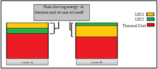
Figure 1.
Selected thermal unit that peak shaved its energy from several optimized limited energy units (LEUs) having different affected order.
In conclusion, the conventional optimization of the PPS technique is not economically feasible, due to some optimized LEU not being able to fully utilize their energy. It is worth mentioning that the artificial intelligent optimization technique was not introduced yet for ODLEU based on the probabilistic method; therefore, the ODLEU using the PPS technique has formulated the issue into a multimodal optimization problem to overcome its weakness. The performance of the Artificial Bee Colony (ABC) algorithm is considered a better or similar to several metaheuristic methods such as Particle Swarm Optimization (PSO) and Genetic Algorithm (GA). This is because the ABC algorithm has few control parameters, strong robustness, fast convergence, and high flexibility [49,50]. However, sometimes, the accuracy of the optimal value cannot meet the requirements due to its disadvantages of premature convergence in the later search period. Karaboga and Akay proposed an improved version of the basic ABC algorithm called the modified ABC (MABC) algorithm, while providing a better convergence property for constrained and real-parameter optimization problems. Although the MABC optimization algorithm has more control parameters, the convergence rate is considered to be better compared to the basic ABC algorithm [51]. As far as the author’s knowledge is concerned, the obtained optimal value of SUC based on ODLEU using the PPS technique and assisted with intelligence techniques has not been examined so far. Therefore, this paper focuses on providing a proposal for the SUC estimation problem by exploiting this optimization algorithm. For this purpose, determining the optimal value of SUC based on the MABC algorithm is designed in this study. The designed estimator is comprehensively analyzed for different scenarios to obtain the optimal value of SUC. In addition, all results were obtained by an unbiased comparison between the SUC determined directly by the MABC-NSM technique and the SUC indirectly assessed by reference to the energy reduction of the thermal units determined using the MABC-NSM. The proposed MABC-NSM method is also compared with the standard ABC. The results obtained showed that the performance of the proposed MABC-NSM is higher than that of standard ABC algorithms concerning the optimal SUC value. Therefore, the proposed MABC-NSM can utilize the LEUs efficiently and gain more profit for electrical utilities.
The remainder of this paper is organized as follows: Section 2 presented the concepts of the PPS technique, including equations, parameters necessary as input to the subsequent optimization procedure, and the determination of SUC. The proposed MABC-NSM algorithm for the estimation of the SUC is presented in Section 3, and Section 4 provides results and discussion. Finally, Section 5 provides the conclusion and outlines possible directions for future research.
2. Determination of SUC Based on PPS Technique
This section briefly discusses the implementation of the PPS technique, which is the key requirement for the determination of PPC and total expected start-up cost (TESC) of the generation system so that the SUC could be obtained by fully utilizing the energy of LEU.
2.1. Determination of Probabilistic Production Cost
The main task of the PPS technique is that the LEU will transfer the maximum amount of its increment energy (Er) to peak shave some of the energy that should be produced by the thermal unit. The technique is used to adjust or switch the energy generated between the units having different marginal cost instead of changing the pattern of load demand or reducing the total generated energy. The performance of the PPS technique continues in such a way that the PPC is minimized and the energy produced is matching with the load demand within an acceptable reliability level. However, the expected energy (En) for each generation system is required to be determined according to the initial loading order prior to the PPS procedure. The En can be obtained using Equation (1) by referring to the equivalent load duration curve ELDC(x) as given in Equation (2). The PPC of the generation system based on the initial loading order can be determined using (3).
where T is the total simulation period in hours, pn and qn are the availability and forced outage rate of the capacity of generating units respectively; is the capacity rate of a generating unit, and represent the starting and the end capacity loading point of the generating unit in the system, respectively; n = {1,…, N} is used to represent the total number of all generating units in the system, and Gcostn represents the operation costs specified for the generating unit. It is worth mentioning that the ELDCn-1(x) in Equation (4) is equivalent to the load duration curve (LDC) in the case that (n = 1). The Er of the dispatched LEU is determined based on the difference between generated energy by the selected thermal unit before and after the dispatch of LEU, as shown in (4).
In Equation (4), k is the loading order of selected thermal unit, while and represent the starting and the end capacity loading point of the selected thermal unit involved in receiving the increment energy Er, respectively. The represents the original ELDC obtained from convolving the outage probability of the selected thermal unit with LDC, while is the extra load subtracted from the original ELDC of the same thermal unit, which is obtained from convolving the outage probability of dispatched LEU with the respective ELDC utilized by the thermal unit as given by (5), where m represents the number of off-loading stages of the selected thermal unit.
Determination of the new energy of LEU dispatched to the loading order of the thermal unit subject to its maximum energy limitation, the energy invariance property associated with the increment energy Er value discharged from the same LEU is expressed as shown in (6). It is worth mentioning that expected energies and of the selected thermal unit and dispatched LEU respectively are computed in the initial loading order.
The process of finding the optimal value of increment energy Er continued sequentially under ELDC and the ELDC of the selected thermal unit with an optimal value of Er updated simultaneously. However, if the previously adjusted thermal unit is reselected to receive the increment energy Er, then ELDCk-1(x) is replaced with and the subsequently forced outage rate of the next LEU (pn and qn) and capacity of the next LEU are used in (7) to calculate the new ().
where m is a number of off-loading stages of the selected thermal unit. Then, both the and are applied in (8) to determine the Er based on the next LEU loading order, which is located between the Er based on the previous LEU loading order and the compulsory energy generated by the thermal unit. In the same manner, the Ek and are replaced with new energies and in the same thermal unit and used (6) for the determination of new energy of the subsequent LEU. The optimization process of the LEU continues until all the LEUs are optimized, and then the PPCnew is calculated by (9).
The first item of (9) is the total operation cost of all generating units, excluding the off-loading thermal units affected by Er. The second and third items are the total operation cost of the thermal unit that is off-loaded by Er and the total operation cost of the LEU involved in dispatching the increment energy Er, respectively. n = {1,…, L} is used to represent all generating units, excluding the off-loading thermal units affected by Er and is the compulsory energy generated by the selected thermal unit after off-loading by the LEUs subsequent to the implementation of . Here, n and k = {1,…, } are used to represent the total number of dispatched LEUs. The is the operation cost for the selected thermal unit involved in receiving the increment energy Er and is an operation cost for the LEU involved in dispatching the increment energy Er.
2.2. Determination of Total Expected Start-Up Cost
The total expected start-up cost (TESC) refers to the several expenses incurred in order to start thermal units such as the fuel, manpower, wear and tear, and loss of equipment life caused by frequent cycling [52]. In fact, the increasing variable renewable generation on the electric grid is considered as one of the important factors causing thermal units exposed to frequent start-up operation. Therefore, the electric utility is required to determine the expected frequency of start-up of thermal units (EFS) over an extended period by forecasting the number of times that the load demand makes a transition from below to above levels. By referring to Equations (10) and (11), the TESC base, according to the initial loading order, can be determined using Equation (12).
The equivalent load frequency curve for the generating unit that can be seen in Equation (10) is made up of two independent contributions. The first part of the equation refers to the load transition resulting from convolution between the two load frequency curves (LFCs) in such a way that the pn and qn of capacity of the thermal unit is taken into account. In addition, the second one refers to the switching between failures and repair states. Where is the mean time between failures of the LEU. It is worth mentioning that the ELFCn-1 (x) in Equation (10) is equal to LFC in the case that (n = 1).
Referring to (12), n = {1,…, NT} is used to represent the total number of thermal units in the generation system; the EFSn for each thermal unit over a period T is determined according to [16], and Supcn is the start-up cost of the thermal unit. Similarly, in PPCnew determining, the performance of PPS technique based on ELDC and ELFC continues in such a way that the TESCnew is also minimized. However, obtaining the new EFS of the particular thermal unit (), which is involved in off-loading its compulsory energy by referring to the increment energy Er received from the LEUs, is required. The value is determined based on changes that occur on ELDC and the ELFC of the selected thermal unit. Therefore, and , which have been determined by using (5) and (13) respectively, are used in (14) to calculate the new located at the same loading order of the thermal unit.
In case the selected thermal unit has peak shaved its energy more than one stage (m ≠ 1), the same procedure of PPS technique is applied to determine and by using (15) and (16), respectively.
The TESCnew is determined using (17) once all the dispatch Er values based on the subsequent LEU loading order are optimized. The TESCnew is specified for the entire thermal units, including the selected thermal units involved in receiving the incremental energy, Er, from the LEUs. Here, n = {1,…, R} is used to represent all the thermal units excluding the off-loading thermal units affected by Er, and k = {1, …, } is used to represent the total number of dispatched LEU.
2.3. Determination of Saving Utility Cost
The determination of the SUC is performed without causing changes to the reliability of the generating system due to the constant values for the final convolution of ELDC and ELFC. Generally, the utility will calculate the two aspects of SUC, which are the SEC and SECC whenever there is a possibility for the optimal dispatch of LEU performed in such a way that will satisfy the peak load demand imposed with the lowest possible energy and operating cost. Section 2.1 and Section 2.2 have explained more elaborately the difference in estimating the PPC and values before and after the optimal dispatch of incremental energy from the LEUs, respectively. In this section, the SEC is determined based on the difference between the two cases of PPC, as shown in Equation (18). In a base case condition, the PPC is obtained by using Equation (3) taking into account the base case of ELDC. In the latter case, given in Equation (9), the PPC is obtained based on a new condition of ELDC due to the dispatch of increment energy Er. As for SECC, it is determined based on the difference between the two cases of as given in Equation (19). In the first case, for all of the thermal generating units, the is obtained by taking into account the base case of ELDC and ELFC, which is basically based on Equation (12). In the second case, the as given in Equation (17) is obtained based on all of the thermal units inclusive with the new condition of ELDC and ELFC applied at the particular thermal units involved in peak-shaving or off-loading its compulsory energy by referring to the Er. Eventually, the SUC of generating systems is defined as the summation of the SEC and SECC as expressed in (20). In addition, Figure 2 has shown the procedure of determination of SUC based on the dispatch increment energy Er from several LEUs using the PPS technique.
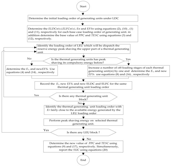
Figure 2.
Flow chart of saving utility cost determination based on dispatch increment energy Er from several limited energy units (LEUs) using the probabilistic peak-shaving technique (PPS) technique.
3. The Proposed MABC-NSM Algorithm for Estimation the SUC
The intelligent foraging behavior of honey bee swarms has inspired toward the development of the ABC algorithm. Contrary to the other optimization algorithms, which mainly rely on probabilistic modeling to change a part of the solution in search of a better solution, the ABC algorithm has the ability to remove an entire unproductive population or Food Source Position (FSP) and randomly initializes a new one to search for better solutions. With this feature, the ABC algorithm shows a better global search ability and proper convergence than another algorithm does [49,50,51,53,54,55]. However, sometimes, the accuracy of the optimal value cannot meet the requirements due to its disadvantages of premature convergence in the later search period. Therefore, this paper proposed a new development approach of the MABC with a new searching mechanism (MABC-NSM) optimization technique constituted with robustness to determine the global optimal solution of the SUC. Section 3.1 and Section 3.2 discuss in detail the random generation of FSP and neighborhood operation of the proposed approach MABC-NSM respectively, which are considered different from the standard ABC algorithm. Eventually, the MABC-NSM algorithm for estimation of the SUC is detailed in Section 3.3.
3.1. Problem Formulation
This section presents the proposed method used to determine the maximum solution for the objective function of SUC, which is considered as a mixed-integer nonlinear programming (MINLP). The aim of solving the SUC problem is to provide an optimal Er dispatched from the LEU to the thermal unit obtained based on the approach of the PPS technique within the framework of the ELDC and FD approach that is assisted by the MABC-NSM optimization method. Section 2 has discussed the PPS methodology used to dispatch a certain amount of increment energy Er from LEU to replace several amounts of energy that are supposed to be produced by the thermal unit and the determination of saving utility cost has also been discussed. The constraint in this case study is generator operating limits, wherein every thermal unit and hydro or LEU has their upper and lower production limits, which can be evaluated by Equations (21) and (22). As for the transmission line, the constraint is not considered due to simplifying computational procedures into the probabilistic simulation. It worth mentioning that the total maximum energy of each LEU is assumed to be given in this case study. Therefore, water discharge constraints and reservoir water storage limits are not necessary to calculate or consider as constraints.
where I and j are indexed for numbers of LEU and thermal units, respectively. is a state variable indicating the energy amount of LEUi that is generated in time period t. In addition, is the state variable indicating the energy amount of the thermal unit j that is generated in time period t.
3.2. Representation of Food Source Position for the Proposed MABC-NSM Algorithm.
This section presents a detailed description of the FSP initialization scheme for the MABC-NSM algorithm to maximize SUC. The FSP is a random selection of thermal units that are selected to perform off-loading or peak shaving to accept increment energy Er dispatched from LEU. Therefore, the total number of randomly selected thermal units is equal to the total number of LEU. It should be noted that a particular thermal unit can be selected more than once, while each LEU can only be discharged once. Hence, the initialization of FSP began with selected the loading order or location () of thermal units by using Equation (23).
where s is the total number of dispatch LEUs, and are the lower and upper bound of the loading order of the selected thermal unit involved in receiving the increment energy Er. Then, the FSP is done by selecting the random position of the thermal unit to receive the Er as shown in Figure 3. The initialized FSP is often used for the initial bee colony (Icol) and scout bee colony (Scol), while on the other hand, the neighboring solution by the MABC-NSM algorithm is required for the employed and onlooker bee colonies.
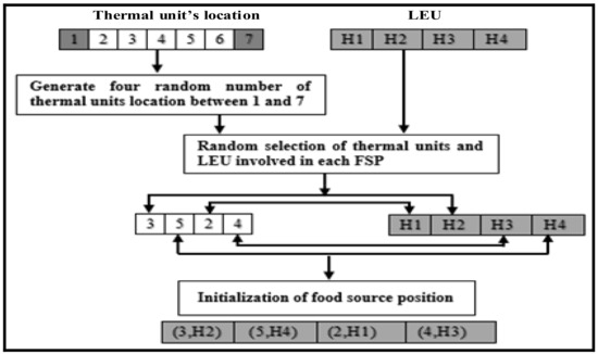
Figure 3.
Initialization of food source position required for initial and scout bee colony .
3.3. Neighborhood Operation for the Proposed MABC-NSM Algorithm.
There is a difference between the NSM algorithm used for each employed bee and onlooker bees for efficient searching ability with low computational time within the neighborhood operation colony (Ncol). The NSM plays a vital role in increasing the search efficiency by preventing the scout bee activation because the best FSP provided by the employed and onlooker bees conveys better information than the random FSP generated by the scout bees during the evolution process [20]. Given that, the employed bee colony (Ecol) is responsible for exploiting available food sources, gathering required information, and sharing it with an onlooker bee colony (Ocol). Thus, each Ecol contains a number of new FSPs which is known as the Ncol. Similar to the initialization of FSP that is discussed in Section 3.1, the thermal units’ loading order (k*) for each Ncol of the best FSP either by the Icol or previous Ecol is updating to produce a new loading order of k** using Equation (23). Then, the FSP is done by simultaneously selecting the random position of thermal unit blocks to receive the Er.
Once all the Ecols have finished with the above exploitation process, they share the information of the FSP with the onlookers. Then, each Ocol selects a food source according to the traditional roulette wheel selection method. After that, neighborhood operation colony (Ncol) is implemented to find the best FSP, and it calculates the nectar amount or the objective function of SUC of the neighbor food source. A similar process occurs in Ocol, but the number of Ncol generated is twice that of Ecol. In the first process, Ncols are generated from the best FSP either by the Ecol or previous Ocol using Equation (24). While in the second process, the Ncols are generated based on Equation (25). The function of Reset is to redo the random selection of the thermal unit and LEU involved in each FSP of the onlooker bee colony. This scheme enhances the searching mechanism of the Ecol and Ocol, thereby reducing the chance of being replaced by the Scol.
In such a way, the neighborhood operation (Ncol) of Ecol and Ocol is performed to explore the optimal solution. However, the Ecol becomes a scout bee colony (Scol) to explore a new solution if the current solution is not improved and reached a limit (a predetermined number). At this point, the newly FSP discovered is memorized, the scout becomes an employed bee again, and simultaneously another iteration of the algorithm begins. The whole process is repeated until a maximum cycle number (MCN) is met.
3.4. The Steps of the MABC-NSM Algorithm
The MABC-NSM is presented as a new approach effectively used to avoid the local optimal trap of SUC solution.
- (a)
- Calculate the base case values of PPCbase and TESCbase using (3) and (12), respectively. Wherein the thermal units are loaded according to merit order, followed by the LEUs arranged corresponding to the decreasing operating hours under the LDC.
- (b)
- Specify the total number of the FSP and Icol required for initialization process.
- (c)
- Specify the total number of Ecol and Ncol required for the NSM process used in the employed bee colony.
- (d)
- Specify the total number of Ocol, Reset, and Ncol required for NSM process used in the onlooker bee colony
- (e)
- Specify the total number of limit (limit) required for activating the Scol.
- (f)
- The initial bee colony (Icol) is implemented in steps (f) until (g), and the SUCIcol is determined using (20) once the two criteria stated earlier and constraints for each dispatched case of in an Icol are met. This is followed by the determination of , , SECIcol, and SECCIcol using (9), (17), (18), and (19), respectively. Repeat the step (f) and simultaneously record all the information that was obtained above until the Icol reached the specified number stated in step (b). Figure 4a has shown all the process of the Icol.
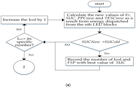
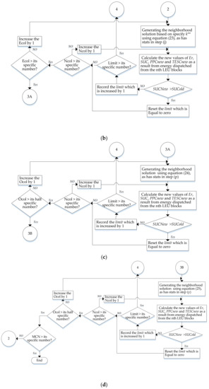
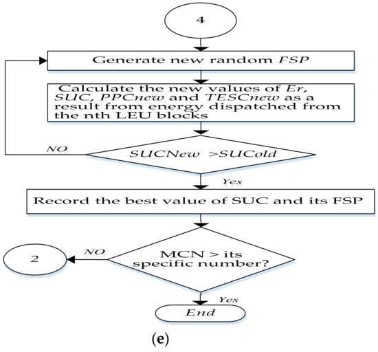 Figure 4. The methodology of the modified artificial bee colony with a new searching mechanism (MABC-NSM) algorithm: (a) Initial bee colony (Icol); (b) NSM-Employed bee colony (Ecol); (c) and (d) NSM-Onlooker bee colony (Ocol) for and respectively; (e) Scout bee colony (Scol).
 - (g)
- Select from the colony with the highest value of SUCIcol.
- (h)
- Apply the NSM for employed bee colony (Ecol), which will provide several Ncols for each particular Ecol derived from obtained from (g). The NSM is implemented in steps (j) until (o) as illustrated in Figure 4b, so that the Ecol can be produced with less probability of being replaced by Scol.
- (i)
- Set the number of Ecol as 1.
- (j)
- Specify k** as the new variables or the locations of the thermal unit using Equation (23) from obtained from step (g) or obtained from step (m).
- (k)
- Determine the SUCNcol, once the two criteria stated earlier and constraints for each dispatched case of in an Ncol are met.
- (l)
- Differentiate between the values of SUCNcol and SUCIcol produced by the and respectively or differentiate between the values of SUCNcol and SUCEcol-1 produced by the and , respectively.
- (m)
- Record the number of Ecol, Ncol, and having the same value as the only when it gives the result of SUCNcol that is higher than the SUCIcol produced by the or SUCNcol is higher than SUCEcol-1 associated with the ; then, the limit is reset to 0 and proceed to step (m(ii)).
- i.
- In contrast to the above matter, when only the SUCNcol is lower than the SUCIcol or SUCEcol-1 , then record the limit which is increased by 1 and perform the subsequent process. Only if the limit has reached the specified number as set in step (e), then stipulate having a similar value as the or obtained from step (g) or (m) and simultaneously proceed to step (aa).
- ii.
- Simultaneously, the subsequent process is performed, which increases the Ncol by 1 and then repeat steps (k)–(m) to produce for a particular Ecol. If Ncol has not reached the total number specified in step (c), otherwise increase the Ecol by 1 and then repeat steps (j)–(m) to produce for a new Ecol. Proceed to step (n) if the Ecol has reached the predetermined threshold given in step (c).
- (n)
- Sort the recorded information of Ecol, , and SUCEcol, which are obtained in step (m).
- (o)
- Choose the final arrangement of the employed bee colony,, including the information of SUCEcol.
- (p)
- Apply the NSM to obtain several onlooker bee colonies (Ocol) originated from an employed bee colony obtained from step (o). The NSM process of the onlooker bee colony encompassed under the steps (r) to (z) is illustrated in Figure 4c.
- (q)
- Increase the Reset by 1.
- (r)
- Specify the number of Ocol as 1.
- (s)
- Define using Equation (24) from the thermal unit of obtained from step (o) or obtained from step (v).
- (t)
- Determine the neighboring colony to calculate the new value of SUC obtained based on the energy dispatched from the LEU to the thermal unit. This implies that the neighboring colony contains the value of yielding the SUCNcol.
- (u)
- Compare the value of SUCNcol and SUCEcol produced by and obtained from step (o), respectively, or the value of SUCNcol and SUCOcol produced by and obtained from step (v), respectively.
- (v)
- Record the number of Ocol, Ncol, and equivalent to once it gives the SUCNcol result that is higher than SUCEcol produced based on the or SUCNcol is higher than SUCOcol-1 associated with simultaneously, the limit is reset to 0 and increase the Reset of the onlooker bee colony by 1. The limit for Reset has been specified in step (d), and then proceed to step (v(ii)).
- i.
- In contrast to the above matter, when only the SUCNcol is lower than the SUCEcol or SUCOcol-1, then record the limit which is increased by 1 and perform the subsequent process. Only if the limit has reached the specified number as set in step (e), then stipulate having a similar value as the or obtained from step (o) or (v) and simultaneously proceed to step (bb).
- ii.
- The subsequent process increases the Ncol by 1 and then repeats steps (t)–(v) to produce for a particular Ocol, if Ncol has not reached the total number specified in step (d); otherwise, increase the Ocol by 1 and then repeat steps (s)–(v) to produce for the new Ocol. If Ncol has reached the total number specified in step (d) then simultaneously proceed to step (w) if Ocol reaches half of the predetermined threshold or limit given in step (d).
- (w)
- Arrange the recorded information of Ocol, , and SUCOcol obtained in steps (v). All the information is obtained based on Ocol in the current Reset.
- (x)
- Select the last row of the onlooker bee colony including the information of Ocol and SUCOcol.
- (y)
- Repeat the NSM for the onlooker bee colony from step (t) until step (w) as shown Figure 4d to produce , and SUCOcol. is obtained using Equation (25) from the thermal unit of obtained from step (x).
- (z)
- Select the last row or arrangement of the onlooker bee colony , including the information of Ocol and SUCOcol.
- (aa)
- Determine a scout bee colony, as shown Figure 4e, if the limit recorded in steps (m)(i) or (v)(i) reaches the limit stated in step (e). This is done by performing step (f) to obtain a scout bee colony and the SUCScol.
- (bb)
- Change the name of to and proceed to step (h) if the limit reaches the limit specified in step (e) and has provided a higher value of SUCscol. This means that has the same value as the . Similarly, SUCIcol has a value equal with SUCScol. If the limit does not reach the predetermined limit given in step (e), then change the name of to and proceed to step (h). This signifies that has the same value as obtained from step (z). Similarly, SUCEcol has the same value with SUCOcol obtained from step (z), respectively.
- (cc)
- Halt the ABC process when the last cycle, the maximum cycle number (MCN), is reached, and then proceed to step (dd). Otherwise, proceed to step (h) to the next iteration process of the ABC technique.
- (dd)
- Report the optimal values of SUC.
4. Results and Discussion
In this section, the test system is first described and then followed by the base case results. The results of SUC are selected based on a detailed comparison of standard ABC and the proposed method of MABC-NSM. Furthermore, the comparison of SUC results using the proposed algorithm MABC-NSM is also detailed through the impartial comparison between the SUC determined directly and the SUC indirectly estimated by referring to the energy reduction of thermal units ERTU.
4.1. Test System Description
A winter week load cycle of modified IEEE RTS-79 having the maximum peak load demand of 2850 MW and 3000 MW is used to validate the proposed method. The test system is modified with an additional 25 MW and 15 MW hydro units as specified in accordance with the standard stated in [56] with start-up cost data from [57] and operating cost data for the generating units [58]. The maximum total energy assigned to the hydro units is assumed to be 18,969 MWh.
4.2. Base Case Results
Table 1 displays results that convey important information, which will be used as a reference for SUC determination expounded in the next subsection. These results are basically obtained based on the framework of the ELDC and FD methods without considering the optimal dispatch of the LEU ODLEU (base case condition) for the peak load demand of 2850 MW and 3000 MW considered in the modified IEEE RTS-79. It is noteworthy that in the base case condition, the thermal units are initially arranged according to the merit order or incremental fuel cost followed by the LEU blocks arranged corresponding to the decreasing operating hours as shown in Table 1. The corresponding final results of PPC are $5,658,196 and $6,343,498 with TESC being $386,426 and $386,387 for peak load demands of 2850 MW and 3000 MW, respectively. In this case study, the ODLEU has no effect on the reliability indices. Thus, it is not included in Table 1.

Table 1.
The results of the base case for all generating units based on peak loads of 2850 and 3000 MW for the modified IEEE RTS-79.
4.3. Comparison of SUC Results Using Proposed Method of MABC-NSM and Standard ABC Method
A comparison is made of the results of SUC obtained from the proposed method of MABC-NSM and the standard ABC method. To ensure an impartial comparison of the performance of both optimization techniques, the determination of SUC and its computation time are used as a reference to obtain the finest parameters setting for the ABC and MABC-NSM techniques. The determination of the finest parameters setting for the ABC and ABC-NSM techniques are performed based on the different peak load demand of 2850 MW and 3000 MW for the modified IEEE RTS-79. In this case study, the parameters settings that are used for this comparison are colony size (Cs), the total number of the limit, and the maximum cycling number (MCN).
4.3.1. Parameter Setting for Cs of ABC and ABC-NSM Techniques
The best value of Cs is determined subsequent to several iterative runs of all the operators embedded in the ABC and MABC-NSM techniques under the Cs = 100, Cs = 200, Cs = 300, and Cs = 400 associated with the total number of limits, which is set as half of the Cs value, as shown in Table 2. Table 2 represents the results of the SUC, and it is a computational time for every optimal solution performed by both techniques with several iterative runs of embedded operators corresponding to different selected values of Cs. For the peak load demand of 2850 MW, it is observed that the optimal maximum SUCs of $268,676 and $288,185 are obtained at Cs = 100 and Cs = 300 with a computational time of 0.25 hour and 1.28 hours for the ABC and MABC-NSM techniques, respectively. Meanwhile, for the peak load demand of 3000 MW, it is observed that the optimal maximum SUC value of $274,171 and $287,865 are obtained at Cs = 100 and Cs = 300 with a computational time of 0.33 hours and 1.37 hours for the ABC and MABC-NSM techniques, respectively. In contrast to the ABC technique, it is obvious that the MABC-NSM technique performed much better in providing the optimal maximum SUC values of $288,185 and $287,865 within 1.28 hours and 1.37 hours at Cs = 300 for the peak load demands of 2850 MW and 3000 MW, respectively. It is important to mention that despite the ABC having a low computation time, it fails to obtain the optimal globe value. Therefore, the MABC-NSM technique is superior to the ABC in providing the optimal maximum results of SUC. The performance of both optimization techniques is improved because the scout bees are deactivated by not transcending the total number of limit that is set as half of the total number of Cs for the purpose of fair comparison. Eventually, it can be observed that Cs = 300 does significantly culminate toward improving the performance of the MABC-NSM technique and hence providing the finest optimal maximum results of SUC for every peak load demand in contrast with the ABC technique. Therefore, the Cs = 300 will be used as a reference for the determination of other parameters settings specified in the MABC-NSM technique.
Table 2.
Results of saving utility cost (SUC) based on different selected values of Cs and its computational time for every optimal solution performed by Artificial Bee Colony (ABC) and MABC-NSM techniques for peak load demands of 2850 MW and 3000 MW.
4.3.2. Parameter Setting of Total Number of Limit for the MABC-NSM Techniques
The suitability of the value prescribed for the total Limit depends on whether it provides a better solution of the SUC considered as the objective function in the MABC-NSM technique at a reasonably low computational time. In relation with the determination of a suitable total Limit, the investigation is performed in such a way that the proposed MABC-NSM optimization process is executed at every value of Limit = 50, Limit = 100, and Limit = 150, taking into account the finest Cs value that is previously determined in Section 4.3.1 as shown in Table 2. The finest total Limit determined by using the MABC-NSM technique is obtained for every peak load demand of 2850 MW and 3000 MW for the modified IEEE RTS-79. By referring to the assessment of all the total Limits determined by using the MABC-NSM technique obtained based on all of the peak load demand, from Table 3, it can be observed that the Limit = 150 can be considered as the best finest total Limit causing the maximum value of SUC= $28,818 per week with a relatively lower computational time of 1.28 hours and SUC = $287,865 per week with a relatively minimum computational time of 1.37 hours, respectively. Furthermore, for all the peak load demands, the Limit = 50 resulted in the worst minimum value of SUC, as shown in Table 3. The main reason is that the number of iterative processes involved in the NSM easily attains or reaches the Limit = 50, which will cause the activation of scout bees for randomly generating the food sources and adversely impact the insufficient searching results of the SUC.
Table 3.
Results of the SUC based on selected values of Cs = 300 and its computation time for every limit specified in MABC-NSM technique for peak load demands of 2850 MW and 3000 MW.
4.4. Results of SUC Obtained Based on Direct Estimation Using the Proposed Method of MABC-NSM
Table 4 represents several results obtained with regard to the objective function of SUC determined by using the MABC-NSM optimization technique, taking into account the PPS technique under the framework of ELDC and the FD approach. In this case study, the best parameters setting embedded with a population size of 300 and Limit = 150 are applied in the MABC-NSM technique to determine the objective function of SUC corresponding to the peak-load demands of 2850 MW and 3000 MW for the modified IEEE RTS-79.
Table 4.
The results of the objective function of the SUC determined by using the proposed method of the MABC-NSM for the peak-load demands of 2850 MW and 3000 MW.
By referring to Table 4, the new values of PPC are $5,377,799 and $6,061,387 with new values of TESC $378,638 and $380,633 for the peak-load demand of 2850 MW and 3000 MW, respectively. Consequently, the maximum SUC values of $288,185 and $287,865 are obtained by the summation of SEC values of $280,397 and $282,111, and SECC values of $7788 and $5754 for 2850 MW and 3000 MW, respectively. From Table 4, it can also be seen that the variations of SEC and SECC arise in such a way that there are changes of En and EFSn that are imminent in the thermal unit affected by the dispatch increments energy of LEU. Moreover, the negative value of SECC and EFSn originated from changes occurs in LFC during the application of ODLEU. Contrary to decreasing the load demand on the selected thermal unit that is shown in column two of Table 4, the number of times that the demand makes a transition from a level below to a level above is increased in comparison with the base LFC condition. The En and EFSn have remained the same for the rest of the thermal unit for the peak-load demands of 2850 and 3000 MW, as shown in Table 1.
4.5. Comparison of SUC Results Obtained Based on Direct Estimation and Indirect by Referring to ERTU
For impartial comparison, the MABC-NSM technique with the finest parameters setting is used to determine SUC directly and indirectly estimated by referring to the ERTU. Section 4.4 has explained in detail the direct estimation of SUC using the MABC-NSM technique with the finest parameters setting. In this section, several results were displayed related to the maximum objective function of ERTU determined by using the proposed method of MABC-NSM. Again, the SUC is reported once all the optimizing LEUs had dispatched based on maximizing ERTU or Er, regardless of the generation operating cost, as shown in Table 5.
Table 5.
Results of SUC estimated indirect by referring the objective function of ERTU based on MABC-NSM for the peak-load demand of 2850 and 3000 MW.
Based on the results shown in Table 4 and Table 5, it is evident that robust performance of the MABC-NSM technique has produced the maximum ERTU of 6248.165 MWh and 5967.510 MWh for the peak load demands of 2850 MW and 3000 MW, respectively. The obtained results of ERTU have achieved 6.27% and 0.97% higher than the ERTU results displayed in Table 4 for the peak load demands of 2850 MW and 3000 MW of the test system, respectively, but the SUC is decreased by 8.49% and 9.16%, respectively. This indicates that dispatched LEUs based on the maximum ERTU is not met with the energy-efficiency concept, nor is it economically feasible. It is important to mention that despite the standard ABC algorithm failing to obtain the optimal globe value of SUC as compared with the MABC-NSM algorithm, it is considered higher than the result obtained based on a maximum of ERTU for all the peak demand. Therefore, the result based on the standard ABC algorithm is used as a reference to measure the efficiency, and it is compared with the MABC-NSM algorithm that is displayed in Table 6.
Table 6.
Comparison of SUC results obtained based on the standard Artificial Bee Colony (ABC) and MABC-NSM algorithm. ERTU: energy reduction of thermal units, PPC: probabilistic production cost, SEC: Saving Energy Cost, SECC: Saving Expected Cycling Cost, TESC: total expected start-up cost.
From Table 6, it can be easily noticed that the proposed MABC-NSM technique is not only limited to directly determine the maximum value of SUC, but also its resilient performance does augment the energy efficiency in terms of the minimum total reduced energy margin for the certain thermal unit peak-shaved by the minimum total Er of the LEU. The proposed MABC-NSM technique has achieved 10.65% and 5.25% of the ERTU higher than the standard ABC technique for 2850 MW and 3000 MW of the test system, respectively. Furthermore, the SUC is increased by 7.26% and 5%, respectively.
5. Conclusions
This paper has expounded in detail on the modified IEEE RTS-79 test systems used as the case study for the comparative analyses on the results of the saving utility cost (SUC) obtained from the ODLEU performed based on different peak load demands. The PPS methodology is assisted with an optimization technique to dispatch a certain amount of increment energy Er from the LEU block to replace several amounts of energy that are supposed to be produced by the thermal unit. This paper has successfully achieved all of the specified objectives, which include developing a new approach of the MABC-NSM optimization technique with robustness to determine the global optimal solution of SUC obtained based on the ODLEU. Herein, the optimal value is selected based on a detailed comparison of standard ABC and the proposed method of MABC-NSM. The achievement of the proposed method is related to composing a new approach of a new searching mechanism that is performed via the process of employed and onlooker bees included under the procedure of the MABC-NSM algorithm. The results have also shown that NSM plays a vital role in increasing the search efficacy by avoiding activating the scout bee. This is because the best food source in the population provided by the employed and onlooker bees often carries better information than the random food source generated by scout bees during the evolution process. The other objective which also has been done successfully is related to obtaining the optimal value of SUC through the impartial comparison between the SUC determined directly by using the MABC-NSM technique and the SUC indirectly estimated by referring to the energy reduction of thermal units determined by using the MABC-NSM. The proposed MABC-NSM technique has achieved ERTU values that are 10.65% and 5.25% higher than the standard ABC technique for the test systems of 2850 MW and 3000 MW, respectively. Furthermore, SUC is increased by 7.26% and 5%, respectively. Nevertheless, the transmission line limit is not taken into account as a constraint in the optimization method, which is used to specify the dispatch of energy from the LEU blocks to several thermal units. Future works certainly will require a transmission line limit that can be considered as one of the constraints in the optimization method used for determining the dispatch of the energy from the LEU blocks to the thermal unit. The proposed optimization method used for determining the dispatch of the energy indeed can be performed based on two case studies that are either referring to a specific area or the entire system. Another recommendation is to develop a new technique based on probabilistic production simulation of the power system for obtaining the accurate saving utility cost assisted with an optimization technique for other renewable energy called non-dispatchable technologies, such as wind turbines and solar.
Author Contributions
Conceptualization, D.S.S.M. and M.M.O.; methodology, D.S.S.M. and M.M.O.; software, D.S.S.M. and M.M.O.; validation, D.S.S.M., M.M.O., and A.E.; formal analysis, D.S.S.M., M.M.O., and A.E.; investigation, D.S.S.M. and M.M.O.; resources, M.M.O.; data curation, M.M.O.; writing—original draft preparation, D.S.S.M. and M.M.O.; writing—review and editing, M.M.O. and A.E.; visualization, D.S.S.M.; supervision, M.M.O.; project administration, M.M.O.; funding acquisition, M.M.O. All authors have read and agreed to the published version of the manuscript.
Funding
The research was funded by the Long-Term Research Grant (LRGS), The Ministry of Education Malaysia for the program titled "Decarbonisation of Grid with an Optimal Controller and Energy Management for Energy Storage System in Microgrid Applications" with the grant numuber 600-IRMI/LRGS 5/3 (001/2019).
Acknowledgments
The authors would like to thank the Research Management Centre (RMC), Universiti Teknologi MARA, Malaysia for the support and facilities provided to conduct this research project.
Conflicts of Interest
The authors declare no conflict of interest.
Abbreviations
The following abbreviations are used in this manuscript
| ABC | Artificial Bee Colony |
| Er | Energy Increment |
| ERTU | Energy Reduction of Thermal Unit |
| ELDC | Equivalent Load Duration Curve |
| En | Expected Energy |
| EFS | Expected Frequency of Start-Up of Thermal Units |
| FD | Frequency and Duration |
| FSP | Food Source Position |
| GA | Genetics Algorithm |
| Icol | Initial Bee Colony |
| LEU | Limited Energy Unit |
| LFC | Load Frequency Curve |
| MCN | Maximum Cycle Number |
| MABC-NSM | Modified Artificial Bee Colony With New Searching Mechanism |
| MINLP | Mixed Integer Nonlinear Programming |
| Ocol | Onlooker Bee Colony |
| O & M | Operation And Maintenance |
| ODLEU | Optimal Dispatch of Limited Energy Unit |
| PPC | Probabilistic Production Cost |
| PPS | Probabilistic Peak Shaving |
| PSO | Particle Swarm Optimization |
| SEC | Saving Energy Cost |
| SECC | Saving Expected Cycle Cost |
| SUC | Saving Utility Cost |
| Scol | Scout Bee Colony |
| TESC | Total Expected Start-Up Cost |
References
- Tang, Y.; Liu, Z.; Li, L. Performance Comparison of a Distributed Energy System under Different Control Strategies with a Conventional Energy System. Energies 2019, 12, 4613. [Google Scholar] [CrossRef]
- Colin, G.; Chamaillard, Y.; Charlet, A.; Nelson-Gruel, D. Towards a friendly energy management strategy for hybrid electric vehicles with respect to pollution, battery and drivability. Energies 2014, 7, 6013–6030. [Google Scholar] [CrossRef]
- Frei, F.; Sinsel, S.R.; Hanafy, A.; Hoppmann, J. Leaders or laggards? The evolution of electric utilities’ business portfolios during the energy transition. Energy Policy 2018, 120, 655–665. [Google Scholar] [CrossRef]
- Barbato, A.; Capone, A. Optimization models and methods for demand-side management of residential users: A survey. Energies 2014, 7, 5787–5824. [Google Scholar] [CrossRef]
- Watson, D.; Rodgers, M. Utility-scale storage providing peak power to displace on-island diesel generation. J. Energy Storage 2019, 22, 80–87. [Google Scholar] [CrossRef]
- Soto, D. Modeling and measurement of specific fuel consumption in diesel microgrids in Papua, Indonesia. Energy Sustain. Dev. 2018, 45, 180–185. [Google Scholar] [CrossRef]
- Kazem, H.A.; Al-Badi, H.A.; Al Busaidi, A.S.; Chaichan, M.T. Optimum design and evaluation of hybrid solar/wind/diesel power system for Masirah Island. Environ. Dev. Sustain. 2017, 19, 1761–1778. [Google Scholar] [CrossRef]
- Clauser, C.; Ewert, M. The renewables cost challenge: Levelized cost of geothermal electric energy compared to other sources of primary energy–Review and case study. Renew. Sustain. Energy Rev. 2018, 82, 3683–3693. [Google Scholar] [CrossRef]
- Okeniyi, J.O.; Atayero, A.A.; Popoola, S.I.; Okeniyi, E.T.; Alalade, G.M. Smart campus: Data on energy generation costs from distributed generation systems of electrical energy in a Nigerian University. Data Brief 2018, 17, 1082–1090. [Google Scholar] [CrossRef]
- Zhu, K.; Li, X.; Campana, P.E.; Li, H.; Yan, J. Techno-economic feasibility of integrating energy storage systems in refrigerated warehouses. Appl. Energy 2018, 216, 348–357. [Google Scholar] [CrossRef]
- Coker, P.; Torriti, J. Energy interactions: The growing interplay between buildings and energy networks. Sustain. Futures Built Environ. 2050 Foresight Approach Constr. Dev. 2018, 2018, 287. [Google Scholar]
- Brouwer, A.S.; van den Broek, M.; Zappa, W.; Turkenburg, W.C.; Faaij, A. Least-cost options for integrating intermittent renewables in low-carbon power systems. Appl. Energy 2016, 161, 48–74. [Google Scholar] [CrossRef]
- Elliston, B.; Macgill, I.; Diesendorf, M. Least cost 100% renewable electricity scenarios in the Australian National Electricity Market. Energy Policy 2013, 59, 270–282. [Google Scholar] [CrossRef]
- Aghahosseini, A.; Bogdanov, D.; Breyer, C. A techno-economic study of an entirely renewable energy-based power supply for North America for 2030 conditions. Energies 2017, 10, 1171. [Google Scholar] [CrossRef]
- Chaianong, A.; Bangviwat, A.; Menke, C.; Darghouth, N.R. Cost–Benefit Analysis of Rooftop PV Systems on Utilities and Ratepayers in Thailand. Energies 2019, 12, 2265. [Google Scholar] [CrossRef]
- EIA U.S. Levelized Cost and Levelized Avoided Cost of New Generation Resources in the Annual Energy Outlook 2016; EIA U.S.: Washington, DC, USA, 2016. Available online: https://www.eia.gov/outlooks/aeo/pdf/electricity_generation (accessed on 22 June 2020).
- Woolf, T.; Malone, E.; Takahashi, K.; Steinhurst, W. Best Practices in Energy Efficiency Program Screening: How to Ensure that the Value of Energy Efficiency is Properly Accounted For. Available online: https://library.cee1.org/content/best-practices-energy-efficiency-program-screening-how-ensure-value-energy-efficiency-proper (accessed on 22 June 2020).
- Kurokawa, K. Energy from the Desert: Feasability of Very Large Scale Power Generation (VLS-PV); Routledge: London, UK, 2014. [Google Scholar]
- Willis, H.L. Power Distribution Planning Reference Book; CRC Press: Boca Raton, FL, USA, 2004. [Google Scholar]
- Aghahosseini, A.; Bogdanov, D.; Barbosa, L.S.; Breyer, C. Analysing the feasibility of powering the Americas with renewable energy and inter-regional grid interconnections by 2030. Renew. Sustain. Energy Rev. 2019, 105, 187–205. [Google Scholar] [CrossRef]
- Osorio-Aravena, J.; Aghahosseini, A.; Bogdanov, D.; Caldera, U.; Muñoz-Cerón, E.; Breyer, C. Transition toward a fully renewablebased energy system in Chile by 2050 across power, heat, transport and desalination sectors. Int. J. Sustain. Energy Plan. Manag. 2020, 25, 77–94. [Google Scholar]
- Nhamo, G.; Nhamo, S.; Nhemachena, C.; Nhemachena, C.R. Africa and the 2030 Sustainable Energy Goal: A Focus on Access to Renewables and Clean Fuels for Cooking. In Scaling up SDGs Implementation; Springer: New York, NY, USA, 2020; pp. 39–57. [Google Scholar]
- Uddin, M.; Romlie, M.F.; Abdullah, M.F.; Halim, S.A.; Kwang, T.C. A review on peak load shaving strategies. Renew. Sustain. Energy Rev. 2018, 82, 3323–3332. [Google Scholar] [CrossRef]
- Olsthoorn, D.; Haghighat, F.; Moreau, A.; Lacroix, G. Abilities and limitations of thermal mass activation for thermal comfort, peak shifting and shaving: A review. Build. Environ. 2017, 118, 113–127. [Google Scholar] [CrossRef]
- Chang, L.; Zhang, W.; Xu, S.; Spence, K. Review on distributed energy storage systems for utility applications. CPSS Trans. Power Electron. Appl. 2017, 2, 267–276. [Google Scholar] [CrossRef]
- Van den Bergh, K.; Delarue, E. Cycling of conventional power plants: Technical limits and actual costs. Energy Convers. Manag. 2015, 97, 70–77. [Google Scholar] [CrossRef]
- Liao, G.-C. A novel evolutionary algorithm for dynamic economic dispatch with energy saving and emission reduction in power system integrated wind power. Energy 2011, 36, 1018–1029. [Google Scholar] [CrossRef]
- Safdarnejad, S.M.; Hedengren, J.D.; Baxter, L.L. Dynamic optimization of a hybrid system of energy-storing cryogenic carbon capture and a baseline power generation unit. Appl. Energy 2016, 172, 66–79. [Google Scholar] [CrossRef]
- Denny, E.; O’Malley, M. The impact of carbon prices on generation-cycling costs. Energy Policy 2009, 37, 1204–1212. [Google Scholar] [CrossRef]
- Mohammed, O.O.; Mustafa, M.W.; Mohammed, D.S.S.; Salisu, S.; Rufa’i, N.A. A systematic approach to evaluating the influence of demand side management resources on the interarea capacity benefit margin. Bull. Electr. Eng. Inform. 2019, 8, 1441–1450. [Google Scholar] [CrossRef]
- Wang, B.; Li, Y.; Watada, J. Supply reliability and generation cost analysis due to load forecast uncertainty in unit commitment problems. IEEE Trans. Power Syst. 2013, 28, 2242–2252. [Google Scholar] [CrossRef]
- Matos, M.; Bessa, R.; Botterud, A.; Zhou, Z. Forecasting and setting power system operating reserves. In Renewable Energy Forecasting; Elsevier: Amsterdam, The Netherlands, 2017; pp. 279–308. [Google Scholar]
- Badami, M.; Fambri, G.; Mancò, S.; Martino, M.; Damousis, I.G.; Agtzidis, D.; Tzovaras, D. A Decision Support System Tool to Manage the Flexibility in Renewable Energy-Based Power Systems. Energies 2020, 13, 153. [Google Scholar] [CrossRef]
- Zhou, B.; Liu, S.; Lu, S.; Cao, X.; Zhao, W. Cost–benefit analysis of pumped hydro storage using improved probabilistic production simulation method. J. Eng. 2017, 2017, 2146–2151. [Google Scholar] [CrossRef]
- Wu, F.F.; Gross, G. In Probabilistic Simulation Of Power System Operation For Production Cost And Reliability Evaluation. In Proceedings of the IEEE International Symposium on Circuits and Systems, Phoenix, AZ, USA, 25–27 April 1977; Institute of Electrical and Electronics Engineers Inc.: New York, NY, USA, 2017; pp. 877–899. [Google Scholar]
- Jin, T.; Zhou, M.; Li, G. Universal generating function based probabilistic production simulation for wind power integrated power systems. J. Mod. Power Syst. Clean Energy 2017, 5, 134–141. [Google Scholar] [CrossRef]
- Malik, A. Simulation of DSM resources as generating units in probabilistic production costing framework. IEEE Trans. Power Syst. 1998, 13, 1528–1533. [Google Scholar] [CrossRef]
- Li, Y.; Zhou, M.; Wang, D.; Huang, Y.; Han, Z. Universal generating function based probabilistic production simulation approach considering wind speed correlation. Energies 2017, 10, 1786. [Google Scholar] [CrossRef]
- Malik, A. Simulating limited energy units within the framework of ELDC and FD methods. Int. J. Electr. Power Energy Syst. 2004, 26, 645–653. [Google Scholar] [CrossRef]
- Jin, L.; Xie, L.; Wang, X.; Shi, W.; Shao, C. In Power system probabilistic production simulation based on equivalent interval frequency distribution including wind farms. In Proceedings of the 2014 International Conference on Power System Technology, Chengdu, China, 20–22 October 2014; pp. 336–342. [Google Scholar]
- Baleriaux, H.; Jamoulle, E.; de Guertechin, F.L. Simulation de l’exploitation d’un parc de machines thermiques de production d’electricite couple a des stations de pompage. Revue E 1967, 5, 225–245. [Google Scholar]
- Manhire, B.; Jenkins, R.T. A new technique for simulating the operation of multiple assigned-energy generating units suitable for use in generation system expansion planning models. IEEE Trans. Power Appar. Syst. 1982, 10, 3861–3869. [Google Scholar] [CrossRef]
- Ding, T.; Bie, Z.; Sun, C.; Wang, X.; Wang, X. In A new framework of probabilistic production simulation of power systems with wind energy resources. In Proceedings of the 2012 3rd IEEE PES Innovative Smart Grid Technologies Europe (ISGT Europe), Berlin, Germany, 14–17 October 2012; pp. 1–7. [Google Scholar]
- Liu, X.; Wang, H.; Zhou, Q.; Hu, B. In Power system probabilistic cost production simulation with wind power penetration based on multi-state system theory. In Proceedings of the 2012 IEEE Power and Energy Society General Meeting, San Diego, CA, USA, 22–26 July 2012; pp. 1–7. [Google Scholar]
- Wang, H.; Liu, X.; Wang, C. Probabilistic production simulation of a power system with wind power penetration based on improved UGF techniques. J. Mod. Power Syst. Clean Energy 2013, 1, 186–194. [Google Scholar] [CrossRef]
- Zhang, H.-y.; Fang, X.; Li, B.-H.; Han, J.-H.; Shen, H.; Yin, Y.-H. Probabilistic production simulation of power systems with large-scale wind and photovoltaic generation. Electr. Power 2012, 45, 73–76. [Google Scholar]
- Zhu, Y.; Jiang, P.; Yang, S. In An optimal capacity allocation scheme for the wind-PV hybrid power system based on probabilistic production simulation. In Proceedings of the 2014 IEEE Conference on Energy Conversion (CENCON), Johor Bahru, Malaysia, 13–14 October 2014; pp. 277–282. [Google Scholar]
- Bai, X.; Wu, H.; Yang, S.; Li, Z. Probabilistic production simulation of a wind/photovoltaic/energy storage hybrid power system based on sequence operation theory. IET Gener. Transm. Distrib. 2018, 12, 2700–2706. [Google Scholar] [CrossRef]
- Karaboga, D.; Basturk, B. A powerful and efficient algorithm for numerical function optimization: Artificial bee colony (ABC) algorithm. J. Glob. Optim. 2007, 39, 459–471. [Google Scholar] [CrossRef]
- Karaboga, D.; Gorkemli, B.; Ozturk, C.; Karaboga, N. A comprehensive survey: Artificial bee colony (ABC) algorithm and applications. Artif. Intell. Rev. 2014, 42, 21–57. [Google Scholar] [CrossRef]
- Brajevic, I.; Tuba, M. An upgraded artificial bee colony (ABC) algorithm for constrained optimization problems. J. Intell. Manuf. 2013, 24, 729–740. [Google Scholar] [CrossRef]
- Malik, A. Determining expected startups of generating units by frequency and duration approach. IEEE Power Eng. Rev. 2002, 22, 57–59. [Google Scholar] [CrossRef]
- He, X.; Wang, W.; Jiang, J.; Xu, L. An improved artificial bee colony algorithm and its application to multi-objective optimal power flow. Energies 2015, 8, 2412–2437. [Google Scholar] [CrossRef]
- Bhullar, S.; Ghosh, S. Optimal integration of multi distributed generation sources in radial distribution networks using a hybrid algorithm. Energies 2018, 11, 628. [Google Scholar] [CrossRef]
- Garcia Nieto, P.J.; Garcia-Gonzalo, E.; Bernardo Sanchez, A.; Menendez Fernandez, M. A new predictive model based on the ABC optimized multivariate adaptive regression splines approach for predicting the remaining useful life in aircraft engines. Energies 2016, 9, 409. [Google Scholar] [CrossRef]
- Subcommittee, P.M. IEEE reliability test system. IEEE Trans. Power Appar. Syst. 1979, 6, 2047–2054. [Google Scholar] [CrossRef]
- Malik, A.S.; Cory, B.J. An application of frequency and duration approach in generation planning. IEEE Trans. Power Syst. 1997, 12, 1076–1084. [Google Scholar] [CrossRef]
- Dam, Q.B.; Meliopoulos, A.S.; Heydt, G.T.; Bose, A. A breaker-oriented, three-phase IEEE 24-substation test system. IEEE Trans. Power Syst. 2009, 25, 59–67. [Google Scholar]


© 2020 by the authors. Licensee MDPI, Basel, Switzerland. This article is an open access article distributed under the terms and conditions of the Creative Commons Attribution (CC BY) license (http://creativecommons.org/licenses/by/4.0/).