Article

Hydrodynamic Effects of Tidal-Stream Power Extraction for Varying Turbine Operating Conditions

by
Lilia Flores Mateos
1,2,3,*,† and
Michael Hartnett
1,2,3,†
1
College of Engineering and Informatics, NUI Galway, H91TK33 Galway, Ireland
2
Ryan Institute, NUI Galway, H91TK33 Galway, Ireland
3
Centre for Marine and Renewable Energy Ireland (MaREI), P43C573 Cork, Ireland
*
Author to whom correspondence should be addressed.
These authors contributed equally to this work.
Energies 2020, 13(12), 3240; https://doi.org/10.3390/en13123240
Submission received: 5 May 2020 / Revised: 15 June 2020 / Accepted: 17 June 2020 / Published: 23 June 2020
(This article belongs to the Special Issue Challenges Towards Sustainable Energy)

Abstract

:
Realistic evaluation of tidal-stream power extraction effects on local hydrodynamics requires the inclusion of the turbine’s operating conditions (TOC). An alternative approach for simulating the turbine’s array energy capture at a regional scale, momentum sink-TOC, is used to assess the impact of power extraction. The method computes a non-constant thrust force calculated based on the turbine’s operating conditions, and it uses the wake induction factor and blockage ratio to characterise the performance of a turbine. Additionally, the momentum sink-TOC relates the changes produced by power extraction, on the velocity and sea surface within the turbine’s near-field extension, to the turbine’s thrust force. The method was implemented in two hydrodynamic models that solved gradually varying flows (GVF) and rapidly varying flows (RVF). The local hydrodynamic effects produced by tidal-stream power extraction for varying the turbine’s operating conditions was investigated in (i) the thrust and power coefficient calculation, (ii) flow rate reduction, and (iii) tidal currents’ velocity and elevation profiles. Finally, for a turbine array that operates at optimal conditions, the potential energy resource was assessed. The maximisation of power extraction for electrical generation requires the use of an optimum turbine wake induction factor and an adequate blockage ratio, so that the power loss due to turbine wake mixing is reduced. On the other hand, the situations where limiting values of these parameters are used should be avoided as they lead to negligible power available. In terms of hydrodynamical models, an RVF solver provided a more accurate evaluation of the turbine’s operating conditions effect on local hydrodynamics. Particularly satisfactory results were obtained for a partial-fence. In the case of a fence configuration, the GVF solver was found to be a computationally economical tool to pre-assess the resource; however, caution should be taken as the solver did not accurately approximate the velocity decrease produced by energy extraction.

Graphical Abstract

1. Introduction

Particularly strong tidal currents are produced by local geographical constrictions such as narrow straits, channels, off headlands, and between islands and landmasses or basins. At these sites, currents are intensified by hydraulic pressure gradients caused by differences in sea-level, and such locations are attractive for exploiting tidal-stream energy. Despite the fact that a tidal-stream turbine implies a less obstructive configuration for local hydrodynamics than tidal barrage structures and tidal lagoons, tidal-stream turbine arrays are deployed to extract high levels of power. Consequently, it is important to investigate the effects of power extraction on local hydrodynamics; furthermore, it is relevant to study the turbine operating conditions and their influence on local hydrodynamics.
The performance of turbines can be investigated analytically with the linear momentum actuator disk theory (LMADT) within open channel flows (LMAD-OCH). This analytical model provides a more realistic insight into tidal-stream turbine performance in coastal areas as the analysis of energy capture includes (i) the constraint effect of the seabed and ocean free-surface on the coastal tidal-stream, (ii) the generation of a mixing region at the turbine scale [1], where energy capture generates a head drop ( h ) over the turbine array, and (iii) the effect of the turbine blockage ratio.
The numerical representation of a turbine is based on the quantification of the momentum extracted. At the regional scale, three main approaches have been implemented to simulate energy extraction from turbine arrays. They are based on: (i) the drag effect of turbines (bed roughness), (ii) the axial component of the thrust force produced by turbines on the flow (momentum sink), and (iii) the numerical implementation of LMAD-OCH. This last approach relates the turbine operating conditions (defined by the blockage ratio and turbine-wake induction factor) to the momentum extracted by the turbine. Additionally, it links the changes produced in velocity and water depth, within the turbine’s near-field extent, due to power extraction (a more detail description is presented in Section 2.2). The blockage ratio, B, is an indicator of the fraction of a channel cross-sectional area occupied by the turbine and the turbine-wake induction factor, α 4 , refers to the velocity rate reduction downstream of the turbine due to wake mixing dissipation at the turbine scale [2,3]. The rate of reduction experienced by the velocity at the turbine with respect to the upstream velocity can be characterised by a turbine’s porosity. A device with low porosity exerts a larger force on the flow, as less fluid passes through the turbine, and consequently, the flow presents a strong magnitude reduction at the turbine and downstream. Meanwhile, a device with high porosity exerts a smaller force on the flow, allowing a larger flow rate that experiences a lower velocity reduction.
The bottom roughness approach accounts for the momentum extracted by the addition of a quadratic bottom friction term at the region where the arrays are located [4,5,6]. Garrett and Cummins [7] identified that in a finite flow, the depth-averaged drag force imparted by the devices on the flow was proportional to the square of the flow rate. This result encouraged the implementation of bottom roughness to represent turbines as a first approximation. However, this method is not able to simulate array configurations such as rows of turbines [8], neither does it account for flow directionality [9]. Furthermore, the total power simulated does not differentiate between the power available to the turbine and the power lost due to wake mixing and frictional forces [2]. This approach has been used to assess the maximum tidal power potential in the Johnstone Strait, BC, Canada [10], and the Minas Passage in Canada [11]. In both situations, the flow reduction and the estimated maximum power extraction are consistent with the analytic theory described by [7]. In the case of the Minas Passage, the work in Karsten, et al. [11] reported that extracting the maximum power produced significant changes to the tidal amplitudes; however, a large percentage of power (35%) can be extracted with a maximum 5% change in the tidal range in the Minas Passage and the Bay of Fundy–Gulf of Maine system. The increase of bed friction to represent marine turbines in small passages was criticised by [8], who indicated that this implementation emulated the effect of constructing a barrage across the Minas Passage.
The momentum sink amends some limitations of the bottom roughness approach by accounting for flow directionality. This is accomplished by adding a sink term to the momentum equations. The sink term has been used to study the hydrodynamical impact of power extraction from turbine arrays in two dimensions for different turbine array layouts [12,13]. The approach was further refined by the incorporation of a turbine area component. The turbine area quantification within the grid enabled the study of hydrodynamical effects of the inter-turbine spacing and far-field hydro-environmental impacts of tidal turbine arrays [14,15,16]. The sink term has also been implemented in nested models to investigate far-field hydrodynamic effects of turbine arrays at higher resolution domains, where turbines were simulated at the turbine diameter scale [17,18,19]. The simulation at this spatial scale provides information on the turbine interactions and, consequently, the hydrodynamic impacts of individual turbines. In terms of three-dimensional simulations, the momentum sink approach has also been adopted in nested models, to investigate the turbine-scale hydrodynamics [20]. The method has also been used in models such as FLUENT, to study energy extraction effects on local flow in two and three dimensions from within the water column in a tidal flow [21]. Additionally, the approach was used to study far-field impacts of tidal power extraction via turbine arrays, such as the effect on the large-scale sediment dynamics, through an idealised headland sand bank formation [22]; the effect on tidal currents in the Tory Channel, New Zealand [23]; and the influence on the hydrodynamics of Ria de Ribadeo (NW Spain) [24]. Finally, the momentum sink has also been implemented in ocean circulation models [25], to investigate the far-field effect of tidal energy extraction on tidal-driven, wind-driven, and density-driven currents, as well as the effects on the temperature and salinity fields in the Bay of Fundy, the adjacent Gulf of Maine, and the western Scotian Shelf. A drawback of the momentum sink is the omission of tidal-streams’ natural boundaries. In coastal areas, tidal-streams are constrained by the seabed and free-surface. The consideration of these boundaries can substantially increase the power extracted from coastal tidal-streams [7,26,27]. This is a consequence of the constraint effect produced by the seabed and free-surface at shallow waters, which enhance the blockage effect, resulting in the increase of the maximum power extractable by the turbine. Additionally, the momentum sink approach calculates the momentum extracted by a device excluding the operating conditions of the turbine.
The operating conditions of the turbine are important for the correct simulation of the force exerted by the turbine on flow. Their inclusion allows a more realistic assessment of the power extracted by the device. The LMAD-OCH theory accounts for the turbine operating conditions in the simulation of momentum extracted by a turbine. This analytical model develops a relationship between upstream and downstream velocities and water depths as a function of turbine operating conditions. This relationship refers to the relative change of water elevation across an array of turbines [28]. A numerical scheme that solves rapidly varying flows is required to solve the velocity and water depth discontinuities produced by power extraction due to the array. The work in Draper [2] and Draper, et al. [27] implemented the LMAD-OCH in a discontinuous Galerkin finite-element scheme. This model is a Godunov type, and sets the relative change of the water elevation as an internal boundary, which is solved as a Riemann problem. This method has been used to assess the tidal-stream potential of turbines configured as a fence in an idealised channel [27]. A similar configuration was implemented in the Pentland Firth, where the extractable power of sub-channels was estimated as a function of the device operating conditions using an optimum wake-induction factor that varied over the neap-spring tidal cycle [29]. The work in Adcock, et al. [29] identified up to a 30% change in tidal currents when using devices with B > 0.4 ; additionally, the power extracted varied between spring and neap tide. Furthermore, the performance of fences deployed in the sub-channels of Pentland Firth was affected by neighboured fences [30]. In this line, the work in Adcock and Draper [31] reported that the limits to the variation in power over the beat period between M 2 and S 2 tidal constituents depended on the relative amplitude of the tides, the natural dynamic balance of the channel, and the relative size of the turbine array. They also investigated the effect of energy extraction on tidal harmonics; for turbines whose properties did not change significantly over a tidal cycle, they identified a magnitude reduction of even harmonics and an effect of odd harmonics, depending on the natural dynamic balance of the channel. On the other hand, the investigation of partial-fence configurations at an idealised coastal headland indicated that the extractable power was reduced by the flow that bypassed the partial-fence when energy was removed. Additionally, the testing of different combinations of blockage ratios and turbine-wake induction factors indicated the existence of different combinations that maximised the power extraction; however, available power was maximised when large values of B and α 4 were used. They also identified an increase in residual shear stress at the seabed and the potential for mixing of suspended material at the coastal headline when energy was extracted. The work in Serhadlıoğlu, et al. [32] investigated the role of turbine operating conditions, array connectivity, and the location of partial-fences at the Anglesey Skerries, off the Welsh coast, in power estimation. They identified that greater power was extracted by the array when it was located close to the Skerries, as the bypass flow was reduced. In terms of the local hydrodynamics disturbance, maximum power extraction did not produce a significant change of M 2 amplitude and phase; however, local changes occurred to the tidal currents close to the turbine arrays. A limitation of this implementation of LMADT-OCH is the use of an expensive computational technique, which constrains the head drop produced by power extraction; this methodology uses a rapidly varying flow solver and shock-fitting technique. Additionally, the pre-specification of the relative change of the water-elevation across an array, required by the numerical scheme, reduces the possibility to represent realistic scenarios.
On the other hand, the work in Flores-Mateos and Hartnett [33] calculated the energy capture by a turbine array combining the sink term approach and the numerical implementation of LMAD-OCH. In this way, the head drop constraint across a turbine array was avoided. Furthermore, the method, referred to as momentum sink-TOC, was implemented in an rapidly varying flow solver using a shock-capturing capability. The shock-capturing model consists of the algebraic combination of a first-order and a second-order upwind schemes. This solution procedure represents a more attractive option in computational terms than the shock-fitting technique because it does not require solving a Riemann problem to compute the discontinuities produced in the flow due to power removal. Solving a Riemann problem represents an expensive procedure in computational terms [34].
A computationally less expensive, as well as less restrictive approach to simulate the energy capture, momentum sink-TOC is used in this research. This approach implements the momentum sink method and the LMAD-OCH theory and enables the characterisation of the turbine performance in terms of the wake induction factor and blockage ratio. The momentum sink-TOC was incorporated in a gradually varying flow (GVF) solver and a rapidly varying flow (RVF) solver; in this way, it was possible to identify the relevance of the model’s solution procedure in the evaluation of the resource. This paper reports on the local hydrodynamic effects produced by tidal-stream power extraction at a regional scale for varying the turbine’s operating conditions by addressing the following points:
  • Influence of the turbine’s wake induction factor in the thrust and power coefficients calculation.
  • Flow rate effect due to power extraction for increasing values of the blockage ratio.
  • Evaluation of plausible ranges of the turbine’s wake induction factor and blockage ratio values and their effect on the local hydrodynamics through the examination of the elevation and velocity profiles.
  • Assessment of the tidal-stream potential energy resource considering optimal conditions of turbine performance.

2. Modelling Approach

2.1. Hydrodynamic Models

The evaluation of the tidal-stream power resource conducted in this paper used the depth integrated velocity and solute transport (DIVAST) model and the shock-capturing version that used a total variation diminishing (TVD) scheme, DIVAST-TVD. The DIVAST model was developed to simulate hydrodynamic, solute, and sediment transport processes in rivers, estuaries, and coastal waters as it incorporated a flooding and drying capability. DIVAST was originally developed by [35], and since then, it has been calibrated extensively, verified against laboratory and field data [36], and extended to investigate hydro-environmental engineering problems [37,38,39,40,41,42]. Meanwhile, the DIVAST-TVD model was introduced by [43], and it was developed to analyse scenarios that require modelling of rapidly varying flow conditions. The extensive verification of the model investigated situations that require the modelling of abrupt changes in the flow regime such as dam-break scenarios, flash floods, and hydraulic jumps [41,42,43,44,45,46]. Finally, the use of DIVAST and DIVAST-TVD was encouraged by the satisfactory performance of the 2D hydraulic simulations documented in the benchmarking of urban flooding simulations [47] and in the evaluation of hydraulic modelling packages [48].

2.1.1. Gradually Varying Flows

In coastal and estuarine flows where vertical accelerations are small in comparison with horizontal accelerations and the flow is well mixed vertically, flows can be described with a two-dimensional depth integrated version of the shallow water Equations (2D-SWEs) [49]. The 2D-SWEs were used to analyse the evolution of tidal-streams through a tidal channel, characterised by small Froude numbers. For simplicity, the Coriolis force and wind stress were omitted in this research. The Coriolis effect could be neglected because the characteristic length of the channel was small enough not to be significantly influenced by the Coriolis force; nevertheless, in larger domains, the consideration of the Coriolis force could lead to a 10% increase of maximum power extraction [50]. An additional consideration was the viscous terms omission in the momentum equation. This enabled the comparison to the analytical solutions of a tidal-fence configuration with a rigid surface [10] and the LMAD-OCH [27]. The governing equations correspond to the continuity equation (Equation (1)) and momentum equations (Equations (2) and (3)):
ζ t + q x x + q y y = 0
q x t + ( β q x 2 H ) x + ( β q x q y H ) y = g H ζ x g q x q x 2 + q y 2 H 2 C e 2 F T x
q y t + ( β q x q y H ) x + ( β q y 2 H ) y = g H ζ y g q y q x 2 + q y 2 H 2 C e 2 F T y
where q x = U H and q y = V H indicate the depth-integrated velocity flux component in the x- and y-direction; t stands for time, and β is the momentum correction factor for a non-uniform vertical velocity profile. The surface elevation change with respect to mean water depth h is represented by ζ , where the total water depth is indicated as H = h + ζ . The bed shear stress is a function of the Chezy roughness coefficient ( C e ) and acceleration due to gravity (g). Finally, F ( F T x , F T y ) indicate the thrust force imparted by the turbine to the tidal-stream.
Regarding the turbulence simulation, the use of the LMAD-OCH theory enabled parametrising the turbine’s wake mixing occurring within the turbines’ near-field extent. Over this length scale, it was assumed that (1) elevation and velocity perturbations due to power extraction occurred and (2) flow passing through the array mixed to and from a smooth vertical profile similar to the upstream profiles [28]. These considerations in addition to the inviscid flow assumption captured the vertical flow variations produced by horizontal mixing effects [51] and enabled the use of the bed shear stress to characterise the turbulence induced by turbine-wake mixing [52]. In this paper, a small bottom drag was used ( C d = 0.0025), and this value was selected because it best approximated the field measurements of velocity and elevation of M 2 tidal currents in the vicinity and far-field of Rathlin Sound [53]. The Chezy coefficient C e is defined as C e = g / C d . The numerical scheme used in this paper to solve gradually varying flows was DIVAST, and this model was validated and extended to investigate the changes in tidal regime and the environmental impact of the turbines’ spacing [13,15,18]. DIVAST was further extended to assess the tidal-stream energy resource with the momentum sink-TOC method [33,54,55]. The model used an alternating direction implicit (ADI) technique to approximate the solution of the governing differential equations. This technique used centred finite differences for time and space derivatives. In addition, the ADI’s semi-implicit scheme implied the splitting of a single time-step solution into two time-steps. As the computation of the solution considered only one dimension for each half time-step, the solution of a two-dimensional matrix was avoided. The final finite difference equations for each half time-step (HFDT) were solved using the method of Gaussian elimination and back substitution [56]. The numerical scheme for the hydrodynamics was second-order and accurate in both time and space, with no stability constraints. This was due to the time-centred implicit character of the ADI scheme [57]. Hereafter, the model used to solve GVS is referred to as ADI.

2.1.2. Rapidly Varying Flows

According to the LMAD-OCH theory, the power extracted by an array of turbines produces rapid changes in the water depth and velocity field across the array, which can be considered as discontinuities. The simulation of sharp gradients within the flow requires a scheme that solves RVF. In turn, the scheme depends on the solution of the conservative form of the 2D-SWEs for the tidal channel. This representation of the equations secures the conservation of mass and momentum after discretisation. This form of the equations is necessary for the numerical method to preserve the correct solution of the strong gradients (shocks) present in the velocity and elevation fields [43,58]. The conservative form of 2D-SWE is obtained by treating H, q x , and q y as independent functions. This requires splitting the pressure gradient term into the flux gradients and source terms [59,60]. Additionally, the local acceleration term of the continuity equation is expressed in the following form because the temporal variation of the mean-water depth (h) is null ζ t = H t . The re-arrangement of the governing equations (Equations (1)–(3)) into the conservative form leads to the following formulation:
D t + E x + G y = S + T
where:
D = H q x q y ,
E = q x β q x 2 H + g H 2 2 β q x q y H ,
G = q y β q x q y H β q y 2 H + g H 2 2 ,
S = 0 g H h x g q x q x 2 + q y 2 H 2 C e 2 F T x 0 ,
T = 0 0 g H h y g q y q x 2 + q y 2 H 2 C e 2 F T y
Using the operator splitting technique, it is possible to solve Equation (4) by finding the solution of the following two one-dimensional hyperbolic equations [43,61]:
D t + E x = S
D t + G y = T
The numerical scheme used in this paper to solve the RVF is DIVAST-TVD; the model uses a shock-capturing technique to solve discontinuities in the flow [43,44] and parallel computing to optimise its performance [62,63]. The model DIVAST-TVD was modified to incorporate the momentum sink-TOC [54,60], and the advantage of using the shock-capturing technique over existent techniques was discussed by [33]. DIVAST-TVD solves the RVF using a combination of the standard MacCormack scheme and the symmetric total variation diminishing (TVD) term [61]. The numerical solution is approximated with the explicit MacCormack scheme, which requires the use of a predictor and corrector step on each of the x-direction and y-direction. The non-physical oscillations are prevented with the TVD term, and this is a symmetric five point added to the corrector step of the MacCormack scheme [43]. The contribution of each scheme changes depending on the flow’s regime, and modelling of sub-critical flows (smooth) requires the TVD second-order scheme. Meanwhile, modelling of a trans- or super-critical flow uses the MacCormack lower order scheme. Hereafter, the model used to solve RVS is referred to as TVD.

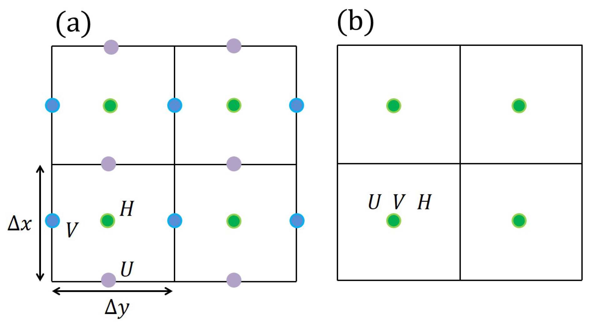
2.1.3. Grid Structures

A finite difference spatial discretisation is used by the ADI and TVD models to approximate the solution of the 2D-SWEs. The equations are discretised onto a square structured grid; however, the models use a different grid structure to compute the solutions (Figure 1). Using the notation introduced by [64], ADI uses a staggered Arakawa C-grid, and TVD uses a non-staggered A-grid. ADI computes and stores the total water depth at the centre of the cell (H); meanwhile, the discharges are discretised on the x- and y-direction as U H and V H , respectively [56,65], as Figure 1a indicates. On the contrary, TVD implements a cell-centred, non-staggered computational grid [43,66]. This procedure indicates that all the variables are stored and computed at the centre of the grid as Figure 1b indicates.
A range of time steps and grid sizes were evaluated to obtain an efficient spatial and temporal resolution, and as a result a spatial discretisation, D X = D Y = 150 m was selected and used in both models. The numerical solution stability of both models was assured by satisfying the Courant–Friedrichs–Lewy condition. Because of the unconditionally stable semi-implicit character of ADI, a constant and larger time step ( t = 12 s) was used. On the other hand, the conditionally stable explicit character of the TVD scheme required a shorter and constant time step ( t = 1.5 s).

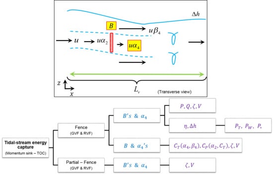
2.2. Turbine-Array Representation

The thrust force applied by arrays of turbines on the tidal-stream was incorporated as an external force F T in the 2D-SWEs momentum equations. The shallow waters model and the convention used to define the water elevation is sketched Figure 2a. The method used to simulate energy capture is called momentum sink-TOC; it is based on the LMAD-OCH theory [2,28] and the momentum sink method [15]. The theory analyses tidal-stream power extraction considering (i) a finite flow constrained by the sea bottom and a free-surface, (ii) a turbine-wake mixing region, and (iii) a length scale where power extraction affects the water depth and velocity, referred to as the turbine’s near-field extent L v (Figure 2b). A more detailed description of L v was given by [33]. LMAD-OCH is also referred to as a turbine-scale model [67] because the quasi-inviscid flow assumption used in the theory allows important turbulent mixing at the array scale to occur at a far downstream region ( L h ) where L v < L h . Consequently, the pressure discontinuity produced by the momentum capture is assumed to be localised, i.e., after momentum extraction, the pressure equalises across the flow. Within the L v region, the quasi-inviscid assumption enables the estimation of the turbine’s thrust force as a function of the changes produced by power extraction in the velocity and water depth. The components of the axial thrust force calculated in the momentum equations and computed by the models per unit grid are:
F T x = 1 x y 1 2 ρ A x C T U 2 F T y = 1 x y 1 2 ρ A y C T V 2
C T is a thrust coefficient, and A indicates the cumulative turbine area per cell-grid computed in the models, where A x is the turbine area projection on the x-direction, and a similar expression is used for the y component. A sketch of F T is presented in Figure 2c.
In the ADI and TVD models, the blockage ratio implemented was the ratio of A over the grid cell cross-section area ( H X ) [54]. The thrust coefficient C T was calculated as a time-varying parameter, which required the selection of a wake-induction factor ( α 4 ) and the estimation of a bypass-induction factor ( β 4 ) as follows: C T = β 4 2 α 4 2 .
Taking as a reference of undisturbed flow the velocity and water depth far upstream the turbine, the power extraction produced an (i) increase in the turbine’s bypass velocity that was characterize by β 4 , (ii) a velocity reduction consequence of energy extraction denoted by the turbine-velocity coefficient α 2 , and (iii) a further velocity reduction consequence of the turbines’ wake mixing dissipation downstream the turbine indicated by α 4 . Factor α 4 is a measure of the turbine’s drag, thereof 0 < α 4 < 1 . Thereof, the parameters that characterised the changes produced in the tidal-stream, within the turbine’s near-field, due to power extraction were: β 4 , α 2 , α 4 , and the water drop h ; where β 4 > 1 and 1 > α 2 > α 4 0 . In particular, the bypass-induction factor is a physical solution of a quartic polynomial [27], which was solved numerically with an Eigenvalue method. According to the LMAD-OCH theory, the turbine-velocity coefficient is solved using the following relation.
α 2 = 2 ( β 4 + α 4 ) ( β 4 1 ) 3 ( B β 4 2 B β 4 α 4 ) 1 4 + ( β 4 2 1 ) ( α 4 β 4 ) 1 .
Identification of α 2 allows the calculation of the power coefficient as C P = α 2 ( β 4 2 α 4 2 ) , and the dependency of C P on these parameters points out the relevance of the turbine operating conditions on the energy extraction process.

2.3. Domain and Array Configuration

The study site was an idealised narrow channel, connecting two large basins (Figure 3); the channel is 12 km long (L) and 3 km wide (W), and the domain presented a constant 40 m depth. From quiescent initial conditions, the domain was forced with a steady M 2 constituent tidal-stream, and the flow conditions were obtained at the eighth tidal cycle. The simulations commenced from quiescent initial conditions and the amplitude of the incident standing wave ramped up over two tidal periods. The domain size was large enough to ensure that the boundary conditions did not influence the power extraction dynamics. Flow conditions reached at the eighth tidal cycle agreed with the conditions at the fourth tidal cycle; consequently, results from the short period are presented. Two turbine configurations were tested and deployed in the middle of the channel. These turbine’s arrays corresponded to a fence and a partial-fence. The fence indicated an array distributed as a single row that fully extended across the cross-section of the channel. The partial-fence covered only 40% of the cross-section; this length was equivalent to 1200 m.

3. Hydrodynamic Effects of Power Extraction

In the absence of turbine deployment, the tidal currents within a channel ( 0 < X < L ) (see Figure 3) experience a velocity increase and a head drop due to the geometrical constraints of the channel. However, tidal-stream energy extraction further affects the channel hydrodynamics. This side-effect is studied in this paper by considering three aspects: wake induction factor ( α 4 ), blockage ratio (B), and turbine array configuration. The six scenarios being discussed in the following sections are presented in Table 1. For a fence configuration, two scenarios were considered: a blockage ratio increasing, for a turbine that operates at optimal power extraction conditions, and a wake induction factor variation, for a specific blockage ratio. In the case of a partial-fence scenario, only the variation of blockage ratio was considered.

3.1. Wake-Induction Factor

The sink term computation required the specification of a turbine wake-induction factor. To determine an optimal α 4 that maximised the power coefficient, the variation effect of 0 < α 4 < 1 was evaluated via Scenarios 2 and 5 (Table 1). These experiments considered a fence configuration and constant blockage ratio B = 0.2 . Figure 4 presents the time-average of the thrust and power coefficients obtained from the wake-induction factor variation for a range of plausible values 0 < α 4 < 1 . These results were obtained with both the ADI and TVD schemes. Figure 4 indicates that the models reported consistent results. This indicated that the solutions obtained from both models for the turbine-velocity coefficient α 2 and the bypass-induction factor β 4 were similar, and therefore, the parametrisation of the tidal-stream velocity changes due to power extraction, at the turbine near-field extent, was consistent in both models. Larger values of C P ¯ fell within the range 0.28 < α 4 < 0.46 , and the maximum value corresponded to α 4 = 0.37 ; consequently, the value selected for the wake induction factor was α 4 = 1 / 3 . The identification of an optimum α 4 enabled the calculation of a thrust and power coefficients that maximised the power extracted for electrical generation. On the contrary, negligible values of C P ¯ were found at the limiting values of the turbine’s wake induction factor. For the condition α 4 0 , the thrust coefficient was high; however, nil power was available for electricity generation, as this limit indicated a turbine with low porosity, which produced a strong velocity reduction linked to a large energy dissipation due to the turbine’s wake mixing. Consequently, the power extracted was being lost. On the other hand, the condition α 4 1 indicated a small thrust coefficient and a negligible available power for electrical generation. This limit corresponded to a high porosity turbine that extracted insignificant power and consequently generated a small velocity reduction and little energy dissipation.

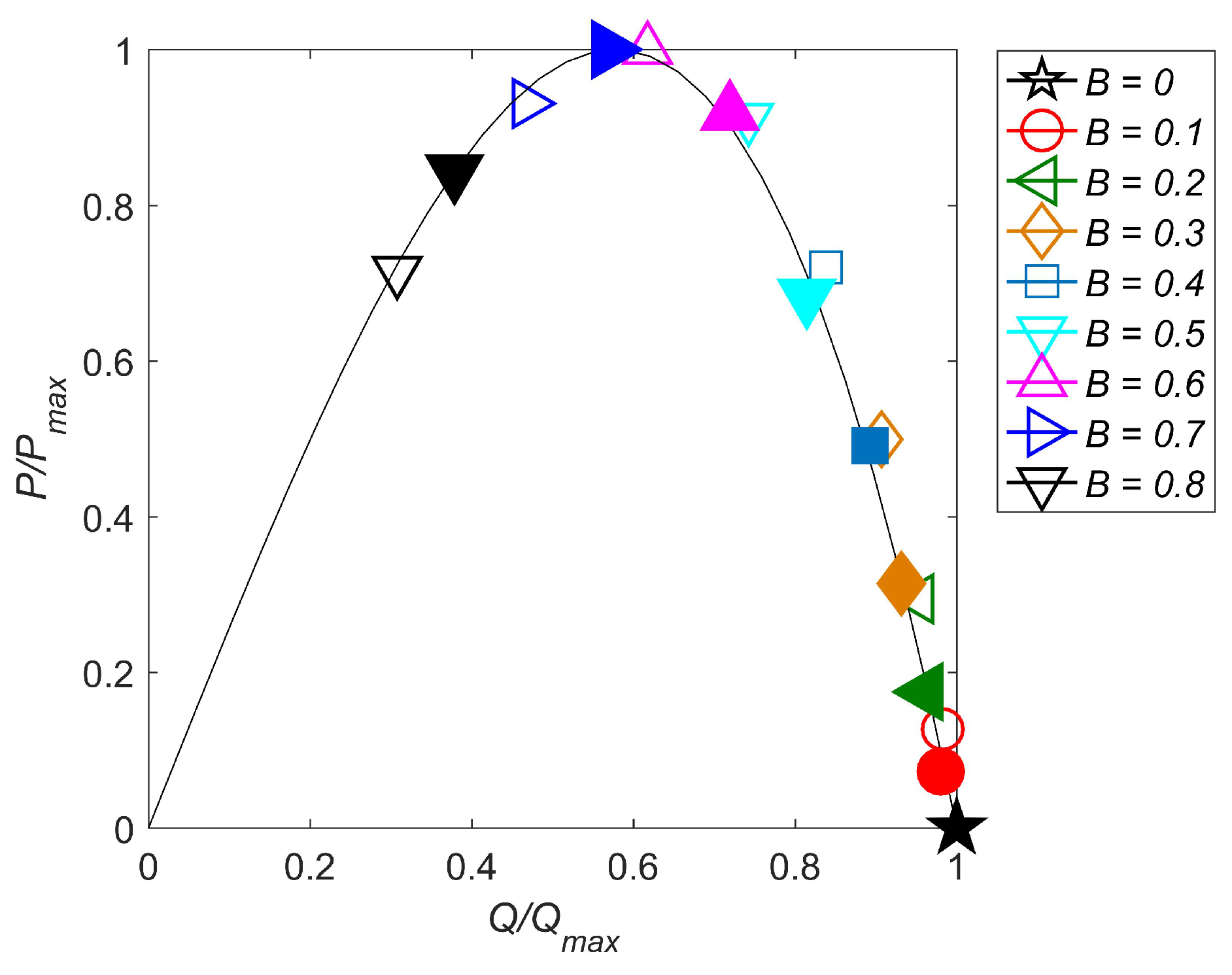
3.2. Power Extraction and Flow Rate Affectation

The maximum power removed by the turbine P was estimated by considering optimum conditions of power extraction and a turbine configuration, which reduced the energy loss. Such a configuration corresponded to a fence, which favoured the simulation of a quasi-steady flow by allowing a constant tidal-stream flux along the channel. Consequently, a fence consideration produced a uniform power extraction across the channel, which avoided losses by wake mixing at the array scale.
On the other hand, energy extraction by the turbines produced a flow reduction throughout the channel as turbines increased the total drag in a channel. To identify the effect of power extraction on the tidal-stream flow rate, Scenarios 1 and 4 (Table 1) were analysed, and they referred to the testing of increasing B values ( 0 < B 0.8 ). Power extracted was calculated as P = 1 2 ρ U 3 A C P , and the results obtained from B variation were normalised to the maximum value of the power extracted P m a x . These results were obtained from both models and compared with an analytical estimation of maximum power extracted reported by [10] (Figure 5). For a uniform power extraction across the channel, the condition satisfied by a tidal fence, the work in Sutherland, et al. [10] derived a normalised power extraction described by the following equation:
P P m a x = 3 3 / 2 2 Q Q m a x 1 Q Q m a x 2
where Q indicates the depth average velocity flow per unit grid obtained for every B tested and Q m a x is the maximum flow rate obtained at the natural state. The testing of increasing values of B indicated a tendency consistent with the analytical solutions documented by [7,10]. The tendency described: (i) a natural state (B = 0) where a maximum flow rate occurred and a null power was extracted, (ii) an optimum blockage ratio that extracted the maximum power P M P , (iii) a power and flow rate reduction for consecutive larger blockage ratios as a consequence of flow choking. High blockage ratios produced a significant flow rate reduction due to the blocking effect produced by the reduction of the turbines lateral spacing. Additionally, large thrust turbines are not practical for realistic designs [51] as they could significantly influence tidal hydrodynamics and the mixing and transport processes of the potential site. These effects would occur at the local scale (turbine scale) and at the regional scale ( 10 1 10 6 m) [51].
The maximum power extracted observed in TVD was obtained with B = 0.6, while ADI reported B = 0.7. The smaller blockage ratio required by TVD to reach P M P was consistent with [27]. Furthermore, lower blockage ratios were required to reach P M P in advection-dominated flows [27]. Such flows experience important flow advection as they are not completely balanced by bed friction drag. The channel investigated in this study was semi-narrow, long, and deep, and it is likely that it presented this kind of flow. Additionally, advection-dominated flows are expected to be more accurately simulated by an RVF solver as sharp gradients present at the channel’s entrance (exit) are better approximated by this scheme [55]. On the other hand, the flow rate reduction modelled by ADI and TVD is an accuracy measure of the solution procedure used by the models. According to the analytical solution of [10], reaching the maximum power extracted requires an optimal B, which is related to an ≈40% flow rate reduction. Therefore, if the blockage ratio required to reach P M P is smaller, the flow reduction occurs at a faster rate [55]. The RVF solver requires a smaller B than the GVF solver to reach P M P (Figure 5), indicating that the ADI model computes a flow rate reduction that takes place at a slower flow rate. As the RVF solver approximates more accurately the flow rate reduction than the GVF solver, the higher blockage ratio reported by the GVF (B = 0.7) suggest that the ADI model underestimates the flow rate decrease caused by energy extraction.

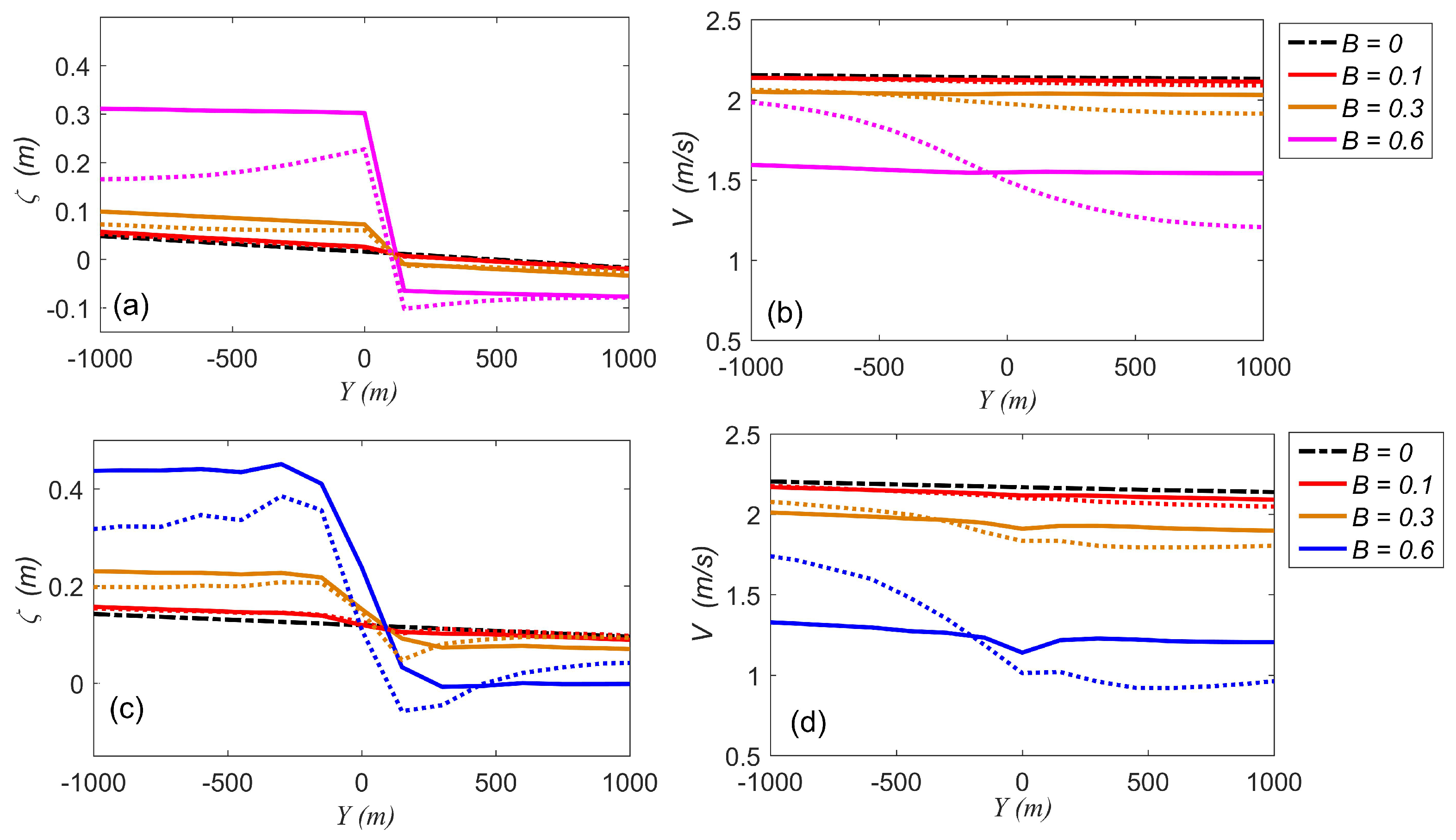
3.3. Wake-Induction Factor Influence on the Tidal-Stream

To better understand the hydrodynamic implications of α 4 , a fence turbine configuration with a local blockage ratio of B = 0.2 was used to evaluate variations of the wake induction factor within a plausible range of 0 < α 4 < 1. The cases analysed corresponded to Scenarios 2 and 5 of Table 1. The flow in the natural state in the middle of the channel was characterised by F r = 0.10 for ADI and F r = 0.11 for TVD. To appreciate the effects of α 4 variations on the tidal-stream, stream-wise profiles of the water elevation ( ζ ) and the Y component of the velocity (V) were analysed. The profiles corresponded to the stream-wise transect that passed along the channel’s centreline, and it is indicated in Figure 6a.
To compare the hydrodynamic effects of α 4 simulated by ADI and TVD, the profiles obtained from both models at flood tide (t = 38.75 h) were normalised to the largest magnitude profile obtained for ζ and V within a 0.3 < Y / L < 1.3 length. In this way, the slightly different flow conditions (defined by F r ) simulated in the natural state by the models were overcome, and a comparison of the results obtained from both models was plausible. In relation to water elevations, the profile with the largest magnitude was obtained as α 4 tended to zero ( α 4 0 ), and the value selected was α 4 = 0.01 . Small values of α 4 indicated a turbine with large drag or low porosity, which produced a strong upstream flow reduction and consequently a high energy dissipation due to turbine-wake mixing. The elevation profiles analysed were normalised to the ζ * profile, which corresponded to the largest magnitude profile for the water elevation and was obtained with α 4 = 0.01 .
Figure 6 shows the elevation profiles normalised by ζ * obtained for two cases: (i) turbine omission and null power extraction and (ii) power extraction with α 4 = 0.01 . The mean water depth corresponded to ζ / ζ * = 0. The results obtained with ADI (Figure 6b,c) and TVD (Figure 6d,e) are reported. The normalised profiles are presented within the 0.3 < Y / L < 1.3 length and a narrow down range of −1000 m < Y < 1000 m. Their extent is indicated in the plan view of the domain in Figure 6a. The 0.3 < Y / L < 1.3 length is represented by a dotted line; meanwhile, the −1000 m < Y < 1000 m length is denoted by a square dashed line, which is also specified by the vertical lines in Figure 6b,d.
Within the 0.3 < Y / L < 1.3 length, the water elevation profiles presented the the following features: (i) high tide on the left basin, (ii) head drop produced by the geometrical constraints of the channel, (iii) water depth drop below the mean water depth near the channel’s exit, and (iv) a water depth discontinuity at the tidal fence location ( Y / L = 0.5 ) when power extraction occurred. These features were observed in the simulations obtained from both models.
Regarding the head drop below mean water ( h e ) , it depended on the channel geometry as the drop was associated with exit separation effects [7], and it was more pronounced in channels with advection-dominated flows [2]. The head loss was of the order of ( | U | ) 2 / 2 g over the region where the cross-section changed from constant to expanded at the channel’s end [7]. The magnitude | U | was the difference in the instantaneous velocity magnitude between the channel’s opening and the uniform section within the channel [2]. Note that in natural state (Nat Sta), the elevation profiles obtained from the models showed a h e that differed in magnitude and location. ADI generated a larger head drop h e located before the channel’s exit, while TVD generated a h e at the exit of the channel. To estimate the dynamical balance of a tidal channel in the natural state accurately, the work in [7,10] suggested the calculation of the phase lag of the current behind the maximum elevation difference in the channel. If the phase lag tended to zero, the pressure gradient forcing was balanced by friction together with separation effects, producing a quasi-steady flow. The phase lags obtained with the models used in this study were 25 (TVD) and 36.5 (ADI), indicating that a quasi-steady flow was better approximated with the TVD modeldue to a better simulation of the balance between the pressure gradient forcing and the channel exit friction effects. Consequently, h e was considered to be better represented by TVD.
The influence of the location of h e in the natural state profiles simulated by the models was illustrated within the −1000 m < Y < 1000 m extent. Here, the fence was situated at Y = 0 . In ADI (Figure 6c), the proximity of h e to the middle of the channel ( Y = 0 ) produced a water depth drop near this location. In the case of TVD (Figure 6e), the closeness of h e to the exit of the channel and, therefore, away from the middle implied a reduced influence of h e on the water elevation at Y = 0 .
Normalised elevation profiles for selected values of α 4 within the −1000 m < Y < 1000 m extent and obtained with ADI and TVD are presented in Figure 7a,c, respectively. Large values of the wake induction factor ( α 4 1.0 ) presented a profile similar to the natural condition state. This small change in elevations was consistent with a turbine with low drag or high porosity, which allows a larger flow rate through the turbine that experiences little losses by turbine wake mixing. Conversely, small values of the parameter ( α 4 0 ) indicated a more pronounced water drop visible as an elevation discontinuity at the location of the fence. These results were consistent with a turbine with large drag or low porosity, which tends to block flow.
In the case of the velocity, the profiles obtained for increasing values of the wake induction factor were normalised to the maximum value of the natural state velocity profile within the −1000 m < Y < 1000 m length, and this value is denoted by V 0 . The solutions obtained with ADI and TVD, along the channel centre, are presented in Figure 7b,d, respectively. The profiles with stronger velocity reduction corresponded to the α 4 0 scenario, and this velocity decrease was associated with a larger dissipation by turbine-wake mixing. The profiles for α 4 1.0 resembled the conditions of a natural state scenario.
The situation that led to optimum power extraction, α 4 1/3, is represented by a thick-blue line in Figure 7. This value of α 4 produced a moderate change on the velocity and elevation profiles, suggesting that the maximisation of power extraction was linked to the reduction of power dissipation by turbine wake mixing.
A comparison of the water depth profiles obtained with both numerical schemes (Figure 7a,c) showed that ADI simulated a smaller head drop across the tidal fence than TVD. The comparison of the velocity profiles (Figure 7b,d) indicated that the simulation of the velocity reduction associated with turbine wake mixing (via the simulation of α 4 1.0 ) was smaller in ADI than TVD. Additionally, the rapidly varying flow scheme generated a more pronounced velocity discontinuity at the array location. In terms of velocity reduction, ADI’s performance was consistent with previous findings, which indicated that the model under-represented velocity reduction. In the case of head drop across the fence, the accuracy of the models to simulate this feature will be discussed in Section 4.1.

3.4. Array Configuration and Blockage Ratio Influence on the Tidal-Stream

A turbine configuration determines the effects power extraction has on tidal-streams. However, the degree of impact depends on the blockage ratio of the turbines within the array. In the case of a fence, as the array completely covers the cross-section of the channel and the flow is bounded by the walls of the channel, the impact of power extraction occurs uniformly across the channel. Conversely, the deployment of a partial-fence implies the existence of an unbounded flow, which only experiences energy extraction in a limited section of the channel cross-section. To account for the hydrodynamic changes produced by the turbine configuration, the blockage ratio range 0 B 0.8 was evaluated for both a fence and a partial-fence. The cases evaluated corresponded to Scenarios 1, 3, 4, and 6 of Table 1. These scenarios considered a flow characterised by F r = 0.11 in the middle of the channel in the natural state.
The impact of increasing B on the tidal-stream was assessed with stream-wise profiles of the Y component of the velocity (V) and the water elevation ζ at t = 38.75 h. These profiles corresponded to a transect that passed along the channel’s centre (Figure 6a). The results obtained from ADI correspond to Figure 8a,b, and the results from TVD are presented in Figure 8c,d. The profiles obtained using a fence are denoted by a continuous line, while profiles obtained from a partial-fence are indicated with a dashed line.
The velocity stream-wise profile obtained with the fence configuration for B = 0.6 showed an almost uniform decrease within the −1000 m < Y < 1000 m length. This uniform velocity effect was also found in smaller blockage ratios such as B = 0.1 , this profile being close to the natural state conditions. In terms of the elevation, ADI (Figure 8a) and TVD (Figure 8c) showed profiles that indicated an increase of the head drop across the fence when larger blockage ratios were implemented. The comparison of the profiles obtained between the models, using a fence configuration, indicated that the elevation profile in the natural state simulated by ADI was lower than TVD. For the power extraction scenario, velocity profiles simulated by TVD presented a stronger reduction than ADI. Additionally, TVD simulated a larger h .
In the case of a partial-fence configuration, power extraction favours the existence of two regions at the array scale: array-bypass flow and array-wake flow. These regions describe the velocity intensification when bypassing the array and the significant velocity diminution downstream of the array due to individual turbines’ wake mixing. Therefore, the array-wake requires a longer distance to recover than an individual turbine’s wake [9]. Research has been carried out to identify the distance required for a turbine-scale wake to merge; however, the authors are not aware of an array-scale wake extension estimation. The strong velocity reduction reported downstream of a partial-fence is evident in the stream-wise velocity profile presented in Figure 8b,d for both ADI and TVD. Note that the partial-fence produced a velocity reduction in the upstream flow, just before passing through the array. This feature illustrated the influence of a partial-fence on the free-flow as reported by [68,69]. In the particular case of TVD, the effect of the upstream velocity by the power extraction was also evident with the fence configuration. Both models reported a profile with a larger magnitude upstream of the array than downstream. This velocity change between upstream and downstream conditions became more abrupt as a larger B was used. In terms of elevations, ADI (Figure 8a) and TVD (Figure 8c) showed that the partial-fence presented a larger downstream water depth reduction than the fence. The more pronounced water-drop was related to the stronger velocity reduction produced by the array-wake generation. A more detail analysis of the head drop is presented in Section 4.1.

4. Energy Resource Assessment

To assesses the upper limits for tidal-stream energy extraction in a semi-narrow tidal channel, considering an M 2 tidal constituent, a scenario with the optimal performance was selected. This corresponded to fence configuration that operated with a wake-induction factor that balanced a large power extraction with a small loss by energy dissipation: α 4 = 1 / 3 . Additionally, the blockage ratio range evaluated was restricted to 0 < B 0.4 to avoid conditions of small lateral spacing associated with large blockage ratios that favour turbine’s wake merging and bypass flow acceleration [9]. In this way, the generation of significant turbulence downstream the fence, which affects tidal hydrodynamics [51], was reduced.
The energy resource evaluation consisted of calculating and comparing power metrics: total power extracted, power removed in terms of the efficiency, and power dissipated by turbine-wake mixing. These metrics required the estimation of a water depth drop, across the fence produced by energy extraction, and the turbine-efficiency.

4.1. Relative Head Drop and Turbine Efficiency

An additional result of the LMAD-OCH theory is the analysis of the turbine-wake mixing region, which leads to the relative head drop h / h and the turbine efficiency η determination. The analysis of shallow water flows with a free-surface indicated that the momentum lost by the stream generated a head drop. The use of the head drop factor in the power extraction showed that the turbine removed potential energy from the tidal-stream instead of kinetic energy [1].
Head drops over the array were calculated as water depth differences between upstream and downstream locations of the fence. Moreover, head drop analytical solutions obtained from the LMADT-OCH theory were estimated by resolving a cubic polynomial, and this expression was derived by [1] and tested by [33]. The polynomial coefficients are a function of F r , B, and C T , and these parameters were obtained from the TVD model as it approximated more accurately the power extraction and flow rate decrease. In Figure 9a, the time-averaged maximum head drop h m a x calculated from the ADI and TVD models are contrasted with the time-averaged h m a x analytical solution. It shows that larger h m a x were obtained with increasing B. Additionally, ADI solutions were more similar to the analytical solutions. This tendency indicated that if energy was extracted using a fence configuration, the head drop was better estimated with a GVF solver. Such a configuration extracted power uniformly along the cross-section of the channel and restricted the energy dissipated to the one generated only by turbine-wake mixing.
The calculation of the turbine’s efficiency η requires the head drop estimation; η indicates the ratio of the power available for electrical generation to the total power extracted by the turbine; it is an indicator of the turbine’s performance. The turbine’s efficiency can be approximated as η α 2 ( 1 h / 2 h ) for flows with small Froude numbers as F r 2 1 h / h 1 , and a detailed derivation of this metric was provided by [60]. Figure 9b shows the time-averaged turbine efficiencies η ¯ and time-averaged thrust coefficient C T ¯ for increasing B calculated them from the ADI and TVD numerical solutions. Increasing values of both B and C T ¯ were related to a gradual reduction of η ¯ , and this trend suggested that larger blockage ratios led to a greater loss of energy due to the turbine’s wake mixing. Both models presented similar turbine’s efficiencies, but TVD reported slightly larger magnitudes possibly due to the larger h m a x simulated by the model.

4.2. Power Metrics

The identification of the head drop change enabled the estimation of the power lost by turbine-wake mixing P W , which was obtained from the evaluation of the changes in kinetic and potential energy between a turbine’s upstream and a far-downstream location [1]. Combining the power lost in the turbine’s wake P W with the power removed by the turbine P, it was possible to identify the total power extracted by the turbine P T (Equation (15)). By taking into account the measure of the effectiveness of the turbine performance η , it was possible to obtain another expression for the power extracted as a function of the turbine’s efficiency and accessible for electrical generation P * power removed in terms of turbine efficiency and available for electrical generation P * (Equation (16)); a detailed derivation was provided by [60]. Finally, a representation of power loss by turbine-wake mixing is obtained in terms of total power extracted and turbine efficiency P W (Equation (17)):
P T = ρ g U A B h 1 F r 2 1 h / 2 h ( 1 h / h ) 2
P * = η P T
P W = P T ( 1 η )
To compare the analytical solutions derived from the LMAD-OCH theory with the numerical solutions obtained from TVD and ADI, the power metrics were calculated following two approaches. The first approach solved the power metrics using the analytical solution of the head drop across an array (Section 4.1); meanwhile, the second approach solved the metrics using the head drop obtained from the models. Figure 10(a.1) shows the time-averaged P T calculated using the analytical and numerical solutions of h Both analytical and numerical solutions of P T showed a larger amount of power extracted with increasing B. In terms of hydrodynamical models, the P T solution presented by ADI agreed better with the analytical solution of P T because this metric was a function of the head drop, and ADI better solved h m a x over the fence. On the other hand, TVD presented larger magnitudes of P T because this solver overestimated h m a x . Regarding the metrics P * and P W , which are a function of the head drop and the turbine’s efficiency, similar solutions obtained for η from both models suggested that the head drop over the array explained the solutions reported by P * and P W . Figure 10(b.1) and Figure 10(c.1) show the time-averaged analytical and numerical solutions of P * and P W , respectively. They indicated that P * and P W obtained with ADI agreed with the analytical solution because of the better resolution of h m a x by the GVF solver.

5. Discussion and Conclusions

At a regional scale, coastal tidal-streams can be approximated as two-dimensional flows with low Froude numbers, whose potential energy resource can be assessed with depth-averaged shallow water equations. The momentum loss associated with tidal-stream power extraction was simulated with the momentum sink-TOC method, which enabled the calculation of a non-constant thrust force that related the turbine operating conditions to the momentum extracted. This method was based on the LMAD-OCH theory, which incorporated the natural constraints of tidal-streams in coastal areas in the analysis of power extraction. The momentum sink-TOC method was implemented in GVF and RVF solvers, which solved the changes produced in the tidal-stream due to power extraction at the turbine’s near-field extent (bypass flow, core flow, and elevation) satisfactorily [54]. Contrary to GVF, the RVF solver used a shock-capturing scheme to solve the rapid changes produced in the tidal-stream. To examine and quantify the disturbance caused by the turbine arrays’ operation to local hydrodynamics, this paper considered the changes produced in the M 2 tidal constituent by power extraction.
The effect of the turbine’s wake dissipation on the tidal stream was tested with increasing values of the wake induction factor. The limiting values of α 4 indicated adverse scenarios where negligible power was extracted for electrical generation. In the case of scenarios where α 4 0 , a maximum thrust force coefficient was found, and a significant power was potentially extracted; however, most of it was loss due to turbine-wake mixing. These scenarios presented a strong velocity reduction and a significant head drop within the turbine’s near-field extent. Similarly, a poor power extraction for electrical generation was obtained when α 4 1 because this scenario corresponded to a minimum thrust coefficient, which indicated nil power extracted. These scenarios did not present head drops and allowed an undisturbed flow rate. Opposite results were obtained for α 4 = 1 / 3 , which corresponded to the optimal wake-induction factor, and it maximised the power available for electrical generation. However, the optimum value of α 4 is a function of the blockage ratio [32] and changes over a tidal period [29]. To the best of the authors’ knowledge, the effect of the turbine-wake induction factor on the tidal currents’ velocity and elevation profiles has not been reported in the literature; however, the effect of α 4 on the power coefficient and turbine-efficiency reported by [54] suggest that the flow behaviour reported here is reasonable.
On the other hand, the blockage ratio had a stronger effect on the tidal currents’ velocity and elevation profiles than the turbine’s wake induction factor variation for a given blockage ratio. The increase of the blockage ratio led to a maximum power extraction, after which, a further increase in B resulted in smaller power extraction due to the flow choking. This free-stream flow reduction throughout the channel due to the power extraction by an array of turbines is referred to as the turbines’ back effect [70,71]. This is a side-effect of turbines’ operation, and it indicates the increase of the total drag in a channel, resulting in a flow rate reduction. The analysis of the back effect simulated by both models indicated that the GVF solver underestimated the flow rate reduction, pointing out its limitations to approximate the velocity reduction due to power extraction accurately.
In terms of turbine configuration, the impact of a fence and partial-fence configuration on local hydrodynamics was intensified with the augmentation of B. By introducing a uniform thrust force on the flow, the fence configuration produced uniform effects of power extraction on the core- and bypass-flow at the turbine scale, i.e., at the near-field region extent, a result consistent with [27,28]. Conversely, in the case of a partial-fence configuration, new features were generated: an array-bypass flow and and array-wake mixing, indicating the existence of another scale (larger and slower than the turbine scale), referred to as the array scale [72]. The subsequent augmentation of B produced a stronger impact on the turbine’s downstream flow due to array-wake mixing generation.
In terms of resource assessment, a realistic range of the blockage ratio was tested ( 0 < B 0.4 ). Otherwise, the implementation of high blockage ratios within the regional scale could produce substantial changes in current velocities, sediment transport, flushing times, and other geochemical processes [9,51,73]. In the case of a large turbine’s array implementation, the reduction of tidal range and a delay in high and low tides were reported to be more significant for small lateral turbine spacing [15]. A scenario with optimal performance conditions, which maximised the power extractable for electrical generation, was used to assess the upper limit of tidal-stream power potential. The evaluation of power metrics required the estimation of the head drops over the array and the turbine’s efficiencies, which in turn were calculated as functions of the parameters that captured the rapid changes produced by energy extraction on the tidal stream within a near-field extent. The implementation of a fence configuration led to the analysis of a bounded flow situation, where both GVF and RVF solvers produced similar turbine efficiencies for increasing B. A consistent result was obtained by [33] for a long partial-fence. The power metrics P T , P * , and P W were evaluated, and their calculation provided a further description of the resource at a regional scale; conventional methodologies were based on a pre-defined constant thrust coefficient [13,15], which did not provide any information about the power loss by the turbine’s wake mixing dissipation. For a fence configuration, the energy resource assessment was better performed with an GVF solver, because the ADI model solved more accurately the head drops over the fence. Additionally, the computational performance testing of ADI and TVD done by [54] indicated a lower computation cost for ADI, suggesting that this model represented a computationally economical tool to assess bounded flows. However, GVF solvers must be used with caution as they seem to underestimate the velocity reductions produced by energy capture.
The method momentum sink-TOC and the analysis presented could be used to assess potential coastal sites such as (i) tidal channels, for example Shannon estuary in Ireland and Cape Cod Canal in Massachusetts USA, (ii) coastal headlands, (iii) bays surrounded by the continental shelf, (iv) tidal channels formed by an island, and (v) sub-channels.
The conclusions of this work are as follows:
  • The turbine’s operating conditions played an important role in determining the available power for electrical energy generation.
  • The maximisation of power extraction for electrical generation required the use of the optimum turbine-wake induction factor and an adequate blockage ratio, so that the power loss due to the turbine’s wake mixing was reduced.
  • Situations where limiting values of the turbine’s operating conditions are used should be avoided, as they led to negligible power available.
    A low wake induction factor was related to high thrust forces, characterised by low porosity turbines. These conditions produced (i) high downstream turbine-wake mixing and, consequently, a high power loss, (ii) strong velocity reduction, and (iii) significant head drop.
    A high wake induction factor indicated low thrust forces, produced by high porosity turbines. This limit indicated (i) less flow disturbance, (ii) small velocity reduction, and (iii) negligible head drop.
    Large blockage ratios also produced high thrust forces, which reduced the flow rate, intensified the magnitudes of flow bypassing the turbines, and enhanced turbine-wake mixing dissipation, reducing the amount of power extracted by the turbines.
  • An accurate evaluation of the turbine’s operating conditions’ effect on local hydrodynamics was provided by an RVF solver. Particularly satisfactory results were obtained for a partial-fence.
  • For scenarios where power was extracted uniformly across a channel (fence configuration), the GVF solver was a computationally economical tool to assess the resource; however, prudence should be taken as the solver underestimated the velocity reduction produced by power extraction.

Author Contributions

Conceptualization, L.F.M. and M.H.; methodology, L.F.M.; validation, L.F.M.; formal analysis, L.F.M.; resources, M.H.; writing, original draft preparation, L.F.M.; writing, review and editing, M.H.; visualization, L.F.M.; funding acquisition, M.H. All authors have read and agreed to the published version of the manuscript.

Funding

This material is based on works supported by the Science Foundation Ireland under Grant No. 436 12/RC/2302 through MaREI, the National Centre for Marine Renewable Energy Ireland.

Acknowledgments

The authors would like to thank the Science Foundation Ireland, the MaREI Centre, and the Irish Centre for High-End Computing (ICHEC) for the provision of computational facilities and support. This is an extension of the work presented at the International Conference on Energy and Environment Research (ICEER) 2019 and published in Energy Reports.

Conflicts of Interest

The authors declare no conflict of interest.

References

  1. Houlsby, G.; Vogel, C. The power available to tidal turbines in an open channel flow. Proc. Inst. Civ. Eng. Energy 2017, 170, 12–21. [Google Scholar] [CrossRef]
  2. Draper, S. Tidal Stream Energy Extraction in Coastal Basins. Ph.D. Thesis, St Catherine’s College, University of Oxford, Oxford, UK, 2011. [Google Scholar]
  3. Johnson, B.; Francis, J.; Howe, J.; Whitty, J. Computational Actuator Disc Models for Wind and Tidal Applications. J. Renew. Energy 2014, 2014, 172461. [Google Scholar] [CrossRef]
  4. Bryden, I.G.; Grinsted, T.; Melville, G.T. Assessing the potential of a simple tidal channel to deliver useful energy. Appl. Ocean Res. 2004, 26, 198–204. [Google Scholar] [CrossRef]
  5. Bryden, I.G.; Couch, S.J. How much energy can be extracted from moving water with a free surface: A question of importance in the field of tidal current energy? Renew. Energy 2007, 32, 1961–1966. [Google Scholar] [CrossRef]
  6. Blanchfield, J.; Garrett, C.; Wild, P.; Rowe, A. The extractable power from a channel linking a bay to the open ocean. Proc. Inst. Mech. Eng. Part A J. Power Energy 2008, 222, 289–297. [Google Scholar] [CrossRef]
  7. Garrett, C.; Cummins, P. The power potential of tidal currents in channels. Proc. R. Soc. A Math. Phys. Eng. Sci. 2005, 461, 2563–2572. [Google Scholar] [CrossRef]
  8. Serhadlioglu, S. Tidal Stream Resource Assessment of the Anglesey Skerries and the Bristol Channel. Ph.D. Thesis, University of Oxford, Oxford, UK, 2014. [Google Scholar]
  9. Nash, S.; Phoenix, A. A review of the current understanding of the hydro-environmental impacts of energy removal by tidal turbines. Renew. Sustain. Energy Rev. 2017, 80, 648–662. [Google Scholar] [CrossRef]
  10. Sutherland, G.; Foreman, M.; Garrett, C. Tidal current energy assessment for Johnstone Strait, Vancouver Island. Proc. Inst. Mech. Eng. Part A J. Power Energy 2007, 221, 147–157. [Google Scholar] [CrossRef]
  11. Karsten, R.H.; McMillan, J.M.; Lickley, M.J.; Haynes, R.D. Assessment of tidal current energy in the Minas Passage, Bay of Fundy. Proc. Inst. Mech. Eng. Part A J. Power Energy 2008, 222, 493–507. [Google Scholar] [CrossRef]
  12. Ahmadian, R.; Falconer, R.; Bockelmann-Evans, B. Far-field modelling of the hydro-environmental impact of tidal stream turbines. Renew. Energy 2012, 38, 107–116. [Google Scholar] [CrossRef]
  13. Ahmadian, R.; Falconer, R.A. Assessment of array shape of tidal stream turbines on hydro-environmental impacts and power output. Renew. Energy 2012, 44, 318–327. [Google Scholar] [CrossRef]
  14. Hartnett, M.; Nash, S.; Olbert, A.; O’Brien, N. Modelling of Hydro-Environmental Impacts from the Installation of Tidal Stream Devices in the Shannon Estuary; Technical Report; Department of Civil Engineering, National University of Ireland: Galway, Ireland, 2012. [Google Scholar]
  15. Fallon, D.; Hartnett, M.; Olbert, A.; Nash, S. The effects of array configuration on the hydro-environmental impacts of tidal turbines. Renew. Energy 2014, 64, 10–25. [Google Scholar] [CrossRef] [Green Version]
  16. Nash, S.; O’Brien, N.; Olbert, A.; Hartnett, M. Modelling the far field hydro-environmental impacts of tidal farms—A focus on tidal regime, inter-tidal zones and flushing. Comput. Geosci. 2014, 71, 20–27. [Google Scholar] [CrossRef]
  17. O’Brien, N. Development of Computationally Efficient Nested Hydrodynamic Models. Ph.D. Thesis, National University of Ireland, Galway, Ireland, 2013. [Google Scholar]
  18. Nash, S.; Olbert, A.; Hartnett, M. Towards a Low-Cost Modelling System for Optimising the Layout of Tidal Turbine Arrays. Energies 2015, 8, 13521–13539. [Google Scholar] [CrossRef] [Green Version]
  19. Phoenix, A. Development of a Tidal Flow Model for Optimisation of Tidal Turbine Arrays. Ph.D. Thesis, National University of Ireland, Galway, Ireland, 2017. [Google Scholar]
  20. Coppinger, D. Development of a Nested 3D Hydrodynamic Model for Tidal Turbine Impact Assessment. Ph.D. Thesis, National University of Ireland, Galway, Ireland, 2016. [Google Scholar]
  21. Sun, X.; Chick, J.P.; Bryden, I.G. Laboratory-scale simulation of energy extraction from tidal currents. Renew. Energy 2008, 33, 1267–1274. [Google Scholar] [CrossRef]
  22. Neill, S.; Jordan, J.R.; Couch, S.J. Impact of tidal energy converter (TEC) arrays on the dynamics of headland sand banks. Renew. Energy 2012, 37, 387–397. [Google Scholar] [CrossRef]
  23. Plew, D.; Stevens, C. Numerical modelling of the effect of turbines on currents in a tidal channel—Tory Channel, New Zealand. Renew. Energy 2013, 57, 269–282. [Google Scholar] [CrossRef]
  24. Ramos, V.; Carballo, R.; Álvarez, M.; Sánchez, M.; Iglesias, G. Assessment of the impacts of tidal stream energy through high-resolution numerical modeling. Energy 2013, 61, 541–554. [Google Scholar] [CrossRef]
  25. Sheng, J.; Thompson, K.; Greenberg, D.; Hill, P. Assessing the Far Field Effects of Tidal Power Extraction on the Bay of Fundy, Gulf of Maine and Scotian Shelf—Final Report; Department of Oceanography, Dalhousie University: Halifax, NS, Canada, 2012. [Google Scholar]
  26. Whelan, J.I.; Graham, J.M.R.; Peiró, J. A free-surface and blockage correction for tidal turbines. J. Fluid Mech. 2009, 624, 281. [Google Scholar] [CrossRef]
  27. Draper, S.; Houlsby, G.T.; Oldfield, M.L.G.; Borthwick, A.G.L. Modelling tidal energy extraction in a depth-averaged coastal domain. IET Renew. Power Gener. 2010, 4, 545. [Google Scholar] [CrossRef] [Green Version]
  28. Houlsby, G.T.; Draper, S.; Oldfield, M.L.G. Application of Linear Momentum Actuator Disc Theory to Open Channel Flow; Technical Report OUEL2296/08; Oxford University Engineering Laboratory UK: Oxford, UK, 2008. [Google Scholar]
  29. Adcock, T.A.A.; Draper, S.; Houlsby, G.T.; Borthwick, A.G.L.; Serhadlioglu, S. The available power from tidal stream turbines in the Pentland Firth. Proc. R. Soc. A Math. Phys. Eng. Sci. 2013, 469, 20130072. [Google Scholar] [CrossRef] [Green Version]
  30. Draper, S.; Adcock, T.A.A.; Borthwick, A.G.L.; Houlsby, G.T. Estimate of the tidal stream power resource of the Pentland Firth. Renew. Energy 2014, 63, 650–657. [Google Scholar] [CrossRef]
  31. Adcock, T.A.A.; Draper, S. Power extraction from tidal channels—Multiple tidal constituents, compound tides and overtides. Renew. Energy 2014, 63, 797–806. [Google Scholar] [CrossRef]
  32. Serhadlıoğlu, S.; Adcock, T.A.A.; Houlsby, G.T.; Draper, S.; Borthwick, A.G.L. Tidal stream energy resource assessment of the Anglesey Skerries. Int. J. Mar. Energy 2013, 3–4, e98–e111. [Google Scholar] [CrossRef] [Green Version]
  33. Flores Mateos, L.; Hartnett, M. Incorporation of a Non-constant Thrust Force Coefficient to Assess Tidal-stream Energy. Energies 2019, 12, 4151. [Google Scholar] [CrossRef] [Green Version]
  34. Shyue, K.M. An Efficient Shock-Capturing Algorithm for Compressible Multicomponent Problems. J. Comput. Phys. 1998, 142, 208–242. [Google Scholar] [CrossRef] [Green Version]
  35. Falconer, R. Temperature distributions in tidal flow field. J. Environ. Eng. 1984, 110, 1099–1116. [Google Scholar] [CrossRef]
  36. Sparks, T.D.; Bockelmann-Evans, B.N.; Falconer, R.A. Laboratory Validation of an Integrated Surface Water–Groundwater Model. J. Water Resour. Prot. 2013, 05, 377–394. [Google Scholar] [CrossRef]
  37. Gao, G.; Falconer, R.; Lin, B. Numerical modelling of sedimente-bacteria interaction processes in surface waters. Water Res. 2011, 45, 10. [Google Scholar] [CrossRef] [Green Version]
  38. Kadiri, M.; Ahmadian, R.; Bockelmann-Evans, B.; Rauen, W.; Falconer, R. A review of the potential water quality impacts of tidal renewable energy systems. Renew. Sustain. Energy Rev. 2012, 16, 329–341. [Google Scholar] [CrossRef]
  39. Kadiri, M.; Ahmadian, R.; Bockelmann-Evans, B.; Kay, D.; Falconer, R. Impact of Different Marine Renewable Energy Scheme Operating Modes on the Eutrophication Potential of the Severn Estuary. In Proceedings of the 35th IAHR World Congress, Chengdu, China, 8–13 September 2013; pp. 1554–1559. [Google Scholar]
  40. Sparks, T.D.; Bockelmann-Evans, B.N.; Falconer, R.A. Development and Analytical Verification of an Integrated 2-D Surface Water–Groundwater Model. Water Resour. Manag. 2013, 27, 2989–3004. [Google Scholar] [CrossRef]
  41. Ahmadian, R.; Falconer, R.; Wicks, J. Benchmarking of flood inundation extent using various dynamically linked one- and two-dimensional approaches. Flood Risk Manag. 2015, 11, S314–S328. [Google Scholar] [CrossRef]
  42. Kvočka, D.; Falconer, R.A.; Bray, M. Appropriate model use for predicting elevations and inundation extent for extreme flood events. Nat. Hazards 2015, 79, 1791–1808. [Google Scholar] [CrossRef] [Green Version]
  43. Liang, D.; Falconer, R.A.; Lin, B. Comparison between TVD-MacCormack and ADI-type solvers of the shallow water equations. Adv. Water Resour. 2006, 29, 1833–1845. [Google Scholar] [CrossRef]
  44. Liang, D.; Lin, B.; Falconer, R.A. Simulation of rapidly varying flow using an efficient TVD–MacCormack scheme. Int. J. Numer. Methods Fluids 2007, 53, 811–826. [Google Scholar] [CrossRef]
  45. Liang, D.; Lin, B.; Falconer, R.A. A boundary-fitted numerical model for flood routing with shock-capturing capability. J. Hydrol. 2007, 332, 477–486. [Google Scholar] [CrossRef]
  46. Liang, D.; Wang, X.; Falconer, R.A.; Bockelmann-Evans, B.N. Solving the depth-integrated solute transport equation with a TVD-MacCormack scheme. Environ. Model. Softw. 2010, 25, 1619–1629. [Google Scholar] [CrossRef]
  47. Hunter, N.M.; Villanueva, I.; Pender, G.; Lin, B.; Mason, D.C.; Falconer, R.A.; Neelz, S.; Crossley, A.J.; Bates, P.D.; Liang, D.; et al. Benchmarking 2D hydraulic models for urban flooding. Proc. ICE Water Manag. 2008, 161, 13–30. [Google Scholar] [CrossRef] [Green Version]
  48. Neelz, S.; Pender, G. Desktop Review of 2D Hydraulic Modelling Packages; Technical Report SC080035; Department for Environment Food and Rural Affairs: Bristol, UK, 2006.
  49. Falconer, R.A. An Introduction to Nearly-horizontal flows. In Coastal, Estuarial and Harbour Engineers’ Reference Book; Abbott, M.B., Price, W.A., Eds.; Chapman and Hall: London, UK, 1993; Chapter 2. [Google Scholar]
  50. Draper, S.; Borthwick, A.G.; Houlsby, G.T. Energy potential of a tidal fence deployed near a coastal headland. Philos. Trans. A Math. Phys. Eng. Sci. 2013, 371, 20120176. [Google Scholar] [CrossRef] [Green Version]
  51. Adcock, T.A.; Draper, S.; Nishino, T. Tidal power generation—A review of hydrodynamic modelling. Proc. Inst. Mech. Eng. Part A J. Power Energy 2015, 229, 755–771. [Google Scholar] [CrossRef]
  52. Nishino, T.; Willden, R.H.J. Effects of 3-D channel blockage and turbulent wake mixing on the limit of power extraction by tidal turbines. Int. J. Heat Fluid Flow 2012, 37, 123–135. [Google Scholar] [CrossRef]
  53. Perez-Ortiz, A.; Borthwick, A.; McNaughton, J.; Avdis, A. Characterization of the Tidal Resource in Rathlin Sound. Renew. Energy 2017. [Google Scholar] [CrossRef]
  54. Flores Mateos, L.; Hartnett, M. Depth average tidal resource assessment considering an open channel flow. In Advances in Renewable Energies Offshore: Proceedings of the 3rd International Conference on Renewable Energies Offshore (RENEW); Soares Guedes, C., Ed.; Taylor & Francis Group: Abingdon, UK, 2018; p. 10. [Google Scholar]
  55. Flores Mateos, L.M.; Hartnett, M. Tidal-stream power assessment—A novel modelling approach. Energy Rep. 2020, 6, 108–113. [Google Scholar] [CrossRef]
  56. Falconer, R.; Lin, B. DIVAST Model Reference Manual; Report; Cardiff University: Cardiff, UK, 2001. [Google Scholar]
  57. Stelling, G.S.; Wiersman, A.K.; Willemse, J.B.T.M. Practical aspects of accurate tidal computations. J. Hydraul. Eng. 1986, 112, 802–816. [Google Scholar] [CrossRef]
  58. Ming, H.T.; Chu, C.R. Two-dimensional shallow water flows simulation using TVD-MacCormack Scheme. J. Hydraul. Res. 2000, 38, 123–131. [Google Scholar] [CrossRef]
  59. Rogers, B.D.; Borthwick, A.G.L.; Taylor, P.H. Mathematical balancing of flux gradient and source terms prior to using Roe’s approximate Riemann solver. J. Comput. Phys. 2003, 192, 422–451. [Google Scholar] [CrossRef]
  60. Flores Mateos, L. Tidal Stream Energy Assessment with and without a Shock Capture Scheme—Incorporating a Non-Constant Thrust Force Coefficient. Ph.D. Thesis, NUI Galway, Galway, Ireland, 2019. [Google Scholar]
  61. Kvocka, D. DIVAST-TVD User Manual; Technical Report; Hydro-Environmental Research Centre School of Engineering Cardiff University: Cardiff, UK, 2015. [Google Scholar]
  62. Whittaker, P. Modelling the Hydrodynamic Drag Force of Flexible RiparianWoodland. Ph.D. Thesis, Cardiff University, Cardiff, UK, 2014. [Google Scholar]
  63. Kvočka, D. Modelling Elevations, Inundation Extent and Hazard Risk for Extreme Flood Events. Ph.D. Thesis, Cardiff University, Cardiff, UK, 2017. [Google Scholar]
  64. Arakawa, A.; Lamb, V. Computational design of the basic dynamical processes of the UCLA general circulation model. Methods Comput. Phys. 1977, 17, 173–265. [Google Scholar]
  65. Nash, S. Development of an Efficient Dynamically-Nested Model for Tidal Hydraulics and Solute Transport. Ph.D. Thesis, National University of Ireland, Galway, Ireland, 2010. [Google Scholar]
  66. Bellos, V.; Tsakiris, G. Grid coarsening and uncertainty in 2D hydrodynamic modelling. In Sustainable Hydraulics in the Era of Global Change; Erpicum, S., Dewals, B., Archambeau, P., Pirotton, M., Eds.; Taylor & Francis Group: London, UK, 2016; pp. 714–720. [Google Scholar] [CrossRef]
  67. Takafumi, N.; Willden, R.H. The Efficiency Of Tidal Fences: A Brief Review And Further Discussion On the Effect of Wake Mixing. In Proceedings of the ASME 2013 32nd International Conference on Ocean, Offshore and Arctic Engineering, Nantes, France, 9–14 June 2013; p. 10. [Google Scholar]
  68. Vogel, C.; Willden, R.; Houlsby, G. A correction for depth-averaged simulations of tidal turbine arrays. In Proceedings of the 10th European Wave and Tidal Energy Conference, Aalborg, Denmark, 2–5 September 2013. [Google Scholar]
  69. Perez-Campos, E.; Nishino, T. Numerical Validation of the Two-Scale Actuator Disc Theory for Marine Turbine Arrays. In Proceedings of the 11th European Wave and Tidal Energy Conference, Nantes, France, 6–11 September 2015; p. 8. [Google Scholar]
  70. Blunden, L.S.; Bahaj, A.S. Tidal energy resource assessment for tidal stream generators. Proc. Inst. Mech. Eng. Part A J. Power Energy 2006, 221, 137–146. [Google Scholar] [CrossRef]
  71. Garrett, C.; Cummins, P. Limits to tidal current power. Renew. Energy 2008, 33, 2485–2490. [Google Scholar] [CrossRef]
  72. Nishino, T.; Willden, R.H.J. The efficiency of an array of tidal turbines partially blocking a wide channel. J. Fluid Mech. 2012, 708, 596–606. [Google Scholar] [CrossRef]
  73. Bonar, P.A.J.; Bryden, I.G.; Borthwick, A.G.L. Social and ecological impacts of marine energy development. Renew. Sustain. Energy Rev. 2015, 47, 486–495. [Google Scholar] [CrossRef]
Figure 1. Sketches of the horizontal grid structure, alternating direction implicit (ADI) model: staggered grid (a), total variation diminishing (TVD) model: non-staggered grid (b).
Energies 13 03240 g001
Figure 2. Sketches of the 2D shallow waters model (a), the tidal-stream power extraction with an actuator disc in open channel flows model (b), and turbine’s thrust force F T exerted on the incident tidal-stream (c).
Energies 13 03240 g002
Figure 3. Tidal channel with a constant cross-section, which connected two large basins. An array of turbines was deployed in the middle of the channel.
Energies 13 03240 g003
Figure 4. Time-averaged thrust and power coefficients obtained from a plausible range of the wake-induction factor, ADI (x marker), and TVD (square marker).
Energies 13 03240 g004
Figure 5. Normalised maximum power removed by the turbines against the normalised maximum flow rate for increasing values of B. TVD (unfilled markers), ADI (filled markers), and the analytical solution (continuous line). Reproduced from [55] with permission from Elsevier.
Energies 13 03240 g005
Figure 6. Plan view of the channel and stream-wise transect indicator (a). Transverse view of normalised water elevation profiles along the stream-wise transect obtained with ADI (b,c) and TVD (d,e). Nat Sta, natural state.
Energies 13 03240 g006
Figure 7. Selected values of normalised water elevation profiles and the Y component of the velocity along the channel centreline obtained with ADI (a,b) and TVD (c,d).
Energies 13 03240 g007
Figure 8. Stream-wise profile of the water elevation ζ and Y component of the velocity, along the channel centreline, for a fence (continuous line) and partial-fence (dashed line) configuration obtained with ADI (a,b) and TVD (c,d).
Energies 13 03240 g008
Figure 9. Effect of the blockage ratio on the maximum head drop (a) and the turbine’s efficiencies (b); results obtained for a fence configuration. Reproduced from [55] with permission from Elsevier.
Energies 13 03240 g009
Figure 10. Effect of the blockage ratio on P T (a.*), P * (b.*), and P W (c.*). Solutions from the analytical model (filled markers), TVD (dashed line), and ADI (continuous line). Reproduced from [55] with permission from Elsevier.
Energies 13 03240 g010
Table 1. Scenarios simulated and initial parameters’ specification.
ModelConfigurationScenarioB α 4 Δ t (s)
ADIFence1 0 B 0.8 α 4 = 1 / 3 12
2B = 0.20 < α 4 < 112
Partial-Fence3 0 B 0.8 α 4 = 1 / 3 12
TVDFence4 0 B 0.8 α 4 = 1 / 3 1.5
5B = 0.20 < α 4 < 11.5
Partial-Fence6 0 B 0.8 α 4 = 1 / 3 1.5

