Abstract
Knowledge about the driving forces behind greenhouse gasses (GHG) emissions is crucial for informed and evidence-based policy towards mitigation of GHG emission and changing production and consumption patterns. Both national and regional-level authorities are capable of addressing their actions more effectively if they have information about the spatial distribution of phenomena related to the policies they conduct. In this context, the main aim of this paper is to explain the regional differences in carbon intensity in Poland. The differences in carbon intensity between regions and the national average were analysed using index decomposition analysis (IDA). Aggregate carbon intensity for regional economies as well as the carbon intensity of households was investigated. For both levels of analysis: total emissions and emission from households economic development is the key factor responsible for the inter-regional differences in carbon emission per capita. In the case of total emissions, the second important factor influencing these differences is the structure of the national power system, i.e., its concentration and the production of energy from fossil fuels. For households, disposable income per capita is a key factor of differences in CO2 emission per capita between regions. Higher households’ incomes contribute to higher emission per capita, mostly due to the shift in consumption towards more energy- and material-intensive goods. The contribution of energy emissivity is quite low and not as varied as in the case of income. This suggests that policy instruments targeted at the consumption of fuels can be rather uniform across regions, while more developed regions should also be subject to measures supporting less energy-intensive consumption. On the other hand, policy in less developed regions should prevent them from following the path of per capita emissions growth.
1. Introduction
The growing need for policies related to climate change results in demand for adequate knowledge on a variety of aspects related to this problem. One of them is the spatial distribution of phenomena and the driving forces of these differences. Energy production and related emissions, as well as consumption of energy, are diverse in space like all other aspects of socio-economic activity. In Poland, where energy production is heavily dependent on coal as a primary energy source, power plants and energy-intensive sectors tend to concentrate in regions with coal deposits. However, while the diversity of energy intensity of regional economies is a fairly recognized issue, the issue of greenhouse gas emissions at the regional level has emerged as an object of increasing interest for both researchers and politicians for about a decade.
Regional perspective (in terms of regions of a country) is strongly addressed in the European Union’s policy. EU, in line with the Paris Agreement, recognises the role of different stakeholders, including regional authorities in addressing climate change. The European transition to a low-carbon economy, according to the Energy Union strategy [1] is intensively supported within the cohesion and regional policy: In the programming period of 2014–2020, a minimum share of each region’s European Regional Development Fund (ERDF) allocation (20% in more developed regions, 15% in transition regions and 12% in less-developed regions) should be “invested in measures supporting the shift to a low-carbon economy” [2]. In the 2021–2028 funding period, the proposed rules on the ERDF require regions (except for developed regions with the Gross National Income per capita above 100% of the EU average) to allocate a mandatory minimum 30% of the available funds to the greener and low-carbon economy [3]. Moreover, a new instrument—The Just Transition Fund—is proposed as part of the European Green Deal [4]. The new fund is to support EU regions relying on fossil fuels and carbon-intensive industries and, therefore, most affected by the EU’s decarbonization policy. The carbon intensity at the regional level is planned to be a key criterion of the funds’ distribution.
Although important, this issue is not addressed consistently by the Polish central government’s policy. Recent updates of the State Energy Policy [5] and the State Environmental Policy [6] published by the Polish government in 2019 address specific situations and needs of mining regions and less developed regions but refer neither to carbon nor energy intensity of regions. On the other hand, the National Strategy for Regional Development recognizes the need for regional policies to reduce energy use and emission, according to the specific regional characteristics [7].
In Poland, like in many other countries, regional authorities conduct their own development policy, which includes their own development strategies. Regional programmes are the main financial mechanism of these strategies and the main channel for spending ERDF funds. The abovementioned requirements related to the proportion of the funds allocated to the greener and low-carbon economy have to be addressed at the regional level. Therefore, reduction in carbon and energy intensity of the regional economy are often referred to as targets of regional strategies, but information concerning this phenomenon at the regional level is very limited.
A more detailed knowledge on the carbon intensity of regional economies is, therefore, useful to both national and regional authorities, but it is only now, when the relevant data has been made available for Poland: Estimates of total regional GHG emissions were calculated first time for the years 2016–2017 by the National Centre for Emissions Management. This makes it possible to analyse the regional differences in carbon intensity.
In this context, the following research question arises: What are the differences in carbon intensities of regional economies? How different are the variations in the carbon intensity of the whole regional economies and in the group of households? It is suspected that the differences in the carbon intensity of households compared to the national average are lower than in the case of the whole regional economies.
To answer these questions, in this study carbon intensity of Polish regions is investigated and the contribution of the factors according to the Kaya identity is analysed.
2. Literature Review
2.1. Logarithmic Mean Divisia Index Methodology
Identification of the influence of driving forces on a particular variable can be made using various methods, both deterministic and probabilistic. In the field of energy and emissions, decomposition analysis is a widely applied and useful tool (see Pearl for a comprehensive review of causality inference methods [8]).
Decomposition analysis has been widely applied in different fields to explore the contribution of driving forces to the changes of an aggregate indicator: In economics, energy, emissions, and other socio-economic issues. The method was first applied in analyses of energy use and energy intensity, and then, because of its convenient formal properties, it was adopted for emission analyses, especially GHG emissions and other problems. This group of methods comprises a range of variants and different types of analyses: Based on absolute or relative numbers (quantities or intensity indicators); temporal, structural or spatial dimension, decomposition form (additive or multiplicative).
Most of these methods are perfect decomposition techniques, i.e., they do not give rise to residuals. Decomposition techniques with and without residuals are discussed by Ang and Liu [9], and other authors. Temporal analyses are either ex-post analyses but are also used to analyse future emissions reduction in national economies and in individual sectors. They are referred to as retrospective and prospective index decomposition analyses [10]. Considering the type of data under analysis, two main decomposition techniques can be distinguished: Index decomposition analysis (IDA) and structural decomposition analysis (SDA). IDA is based on indexes concerning different objects and at different levels and, therefore, is more flexible in terms of data and adjustability while SDA is built upon input-output models, which limits its applications (see Su and Ang [11]).
As repeated surveys by Ang and co-authors show, the predominant approach to decomposition within the IDA method is based on the Logarithmic Mean Divisia Index (LMDI). This is mainly due to its good formal properties and relatively easy interpretation. A comparison of properties of different index decomposition methods done by Hoekstra and van den Bergh [12] confirms that LMDI, as well as Shapley-Sun decomposition [13], is the only index decomposition methods that have three important formal properties:
- Completeness—a residual equals zero; while most of techniques using arithmetic mean weights leave a residual in the calculations, the LMDI uses a logarithmic mean weight and allows perfect decomposition;
- Factor-reversal and time-reversal—the order of factors and direction of comparison over time do not affect the results;
- Zero value robustness—in case of LMDI, zeroes in the data set are replaced with a small positive number.
An overview of IDA using LMDI, its variations and indications to their use are presented, e.g., by Ang [14]. IDA approaches differ in three dimensions: By type of indicator (quantity or intensity indicator), by decomposition procedure (additive or multiplicative decomposition) and by weighting formula (LMDI-I and LMDI-II). As a result, eight types of IDA are distinguished [14] (Figure 1).
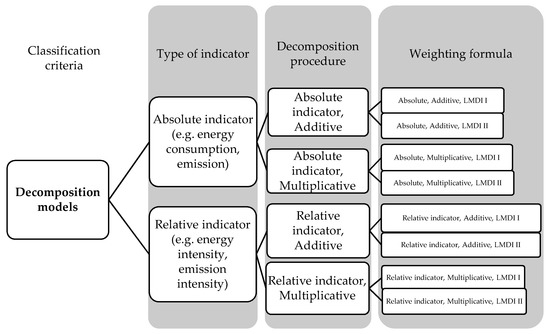
Figure 1.
Eight types of Logarithmic Mean Divisia Index decomposition models. Source: Adapted from reference [14].
In his analysis of desirable attributes of a decomposition method Ang [15], having considered four criteria: theoretical foundation, adaptability, ease of use and ease of result interpretation, suggested LMDI I decomposition as a recommended technique in most applications for energy-related analyses. His considerations also apply to emission analyses.
The choice between LMDI-I and LMDI-II depends on the type of analysis. LMDI-II, apart from its more complicated weighting formula, is not consistent in aggregation and does not allow perfect decomposition at the subcategory level [16]. Therefore, LMDI-I is recommended in the case of subcategory (subsectoral) decomposition and aggregation to the category (sectoral) level. The additive decomposition procedure is recommended for indicators expressed in absolute terms (quantitative indicators), while the multiplicative decomposition procedure is more appropriate for relative indicators (intensity indicators) [14].
Other methodological problems are related to the spatial dimension of analysis. Generally, spatial analyses using IDA methods take two forms. The first one are analyses of differences between regions (in a certain period of time or over time) explaining how different factors influence these differences. This type of analysis is aimed at interregional comparisons of carbon intensity, and, therefore, belongs to the first category. The second form is the decomposition of an aggregate indicator across regions and attribution of changes in an aggregate indicator to individual regions. For this purpose, the attribution analysis method for IDA was proposed by Choi and Ang [17].
Given the question posed in this study, an important issue is how to make spatial comparisons. Generally, cross-regional comparisons can be done in three ways as described by Su and Ang [18]—bilateral-regional (between two regions), radial-regional (between each region in a group of regions) and multi-regional (between regions and a reference object). The choice of comparison method depends on the number of compared units, their type and purpose of analysis. The first type of comparison is by definition possible only if the analysis concerns two objects. If the comparison concerns a larger group of regions, the comparison is more complicated not only because of the number of pairs to be compared. Multi-regional comparisons using LMDI involve a very important methodological problem, i.e., circularity. It is not usually considered an important property in the context of temporal–spatial decomposition [19], but in the case of comparisons between many regions, this property largely determines the method’s optimality and robustness. Since none of the existing IDA methods passes the circularity test (although satisfy the factor-reversal test and leave no residual), multi-regional comparisons should be made using a reference object, as presented e.g., by Ang [19]. To avoid the arbitrariness of choosing a reference object using a group average is suggested [19]. If regions of the world are compared, it is sometimes difficult whereas in the case of comparing regions within one country, it is possible to do so. It is also worth noting that multi-regional comparisons usually deal with relative indicators, as in most cases the objects are of different scale and analysis of absolute numbers would be difficult to interpret [20,21,22]. An important aspect of the analysis of spatial diversity of socio-economic phenomena is also spatial correlation and spillover effects. It is usually assumed that technological progress, foreign direct investments and trade contribute to the gradual decrease in energy and emission intensity, which was confirmed e.g., by Huang et al. [23] and Zhang et al. [24]. This kind of relationship was also revealed for urbanisation [25]. Similar analyses were conducted e.g., for green innovations [26]. However, this type of analysis requires a sufficiently long data series (panel data) to reveal the nature of processes.
2.2. Research Outcomes
Historically, first decomposition analyses dealt with changes in aggregate indicators and quantifying the driving forces behind these changes across a long period of time, like the first study concerning energy consumption in the UK by Bossanyi [27] and many further studies examined by, for example, Ang and his co-authors in a number of review papers [9,28,29]. Spatial decomposition analyses appeared only after 1999, when Ang and Zhang presented their study on comparative analysis of CO2 emissions in North America, Europe and Asia [30]. In their study, like in many others, it was shown that in developed countries the income effect contributes to the higher emission levels, while in less developed countries (in this case the Former Soviet Union and Central and Eastern Europe) much of the positive effect (in terms of CO2 emissions) of the lower-income level is offset by higher aggregate energy intensity. Similar conclusions were drawn e.g., by Kim and Kim [31] or Fernandez-Gonzales et al. [32].
Spatial decomposition analyses concern mainly countries or regions of the world and less attention is paid to the regions within a single country, as confirmed by, e.g., Liu et al. in 2017 [33]. The situation in this respect has not changed much since then. Application of the decomposition analysis method towards regions of a country is limited by data availability and specific regional structure of national economies and energy systems. The largest number of spatial index decomposition analyses on a regional level were conducted on China. Most studies concerning Chinese economy employed the spatial-temporal IDA approach to regional emissions; for example, Liu et al. [33] analysed carbon intensity in Chinese regions from 2000 to 2015, Zhang et al. [21] studied energy-related carbon intensity in Chinese provinces between 1995 and 2012, Song et al. [20] investigated China’s regional carbon intensity from 2000 to 2015, Hang et al. [34] studied SO2 emissions between 2005 and 2015. These studies confirmed in particular that the rapid economic growth in the period 2003–2008 and the resulting growth in energy consumption contributed to higher energy consumption intensity in China. Technological level and energy efficiency of the industry in most provinces of China increased too slow to compensate for growing GDP.
A similar spatial-temporal IDA method was applied not only for energy intensity and emissions, but also for other issues, especially water intensity [22,35,36]. The studies on water intensity in Chinese regions also showed that significant difference in water intensity is accompanied by the difference in the influencing mechanisms of these differences [22,35].
A large part of GHG emission-related studies on households also concerned China [37,38]. Some studies included households as one of the sectors in the decomposition analysis of changes in national emissions e.g., Zhang et al. [39] and Lin et al. [40]. Their studies showed that households had a positive effect on the decrease in the carbon intensity of the economy. In a number of studies, total households emissions were analysed, like Wang et al. who applied an extended STRIPAT model to analyse the scale, structure and driving forces of total carbon emissions from households in 30 provinces of China [38] or Xu et al. who estimated household carbon emissions in one region of China and then examined the influence of a set of demographic, economic, behavioural and spatial factors [41].
Spatial differences in household carbon emissions were mostly analysed using methodologies based on microdata—surveys or household budgets data. For example, Ahmad et al. used household microdata from India’s 60 largest cities and mapped GHG emissions patterns and determinants. They concluded that emissions from direct energy use correlate strongly with income and household size, population density and basic urban services [42]. This also was confirmed within the study of the distribution of household carbon footprint in Great Britain [43], where it was shown that the richest 10 per cent of households emit some three times that of the poorest 10 per cent. These results cannot be directly compared with analyses of the region-level data, but suggest some general trends.
In Europe, IDA has been applied on the country level only, and for cross-country analyses. Index decomposition analyses for European countries regarded: Energy intensity in road freight transport in Spain [44], the energy intensity of European economies [45,46], carbonization index [47] and environmental indicators in general [48]. Structural decomposition analyses were presented, e.g., for the UK by Minx et al. [49] who analysed total emission and by Hammond and Norman who studied energy-related carbon emissions from UK manufacturing [50]. Trends in total CO2 emission were analysed for Germany [51] and air emissions—for Denmark [52].
The very limited number of studies on European countries with a regional dimension concerned decomposition of trends at a regional level. Regional aspects were discussed in a study on electricity consumption in Geneva and Switzerland [53] and in a study by Ivanova et al. [54] on household carbon footprints per capita for 177 regions of the EU-27 (NUTS-1 or NUTS-2 according to the Nomenclature of Territorial Units for Statistics) estimated using multi-regional input-output analysis. The authors of this study conducted regression analysis for a number of variables at household level (income, household size, number of rooms, level of education, urbanisation level).
For Poland, decomposition analysis was very rarely applied in studies concerning emissions. All of them were sectoral-temporal: e.g., a study by Gozdek and Szaruga concerned GHG emission from transport for Poland and Romania [55], study by Iskrzycki et al. [56]—reduction in emission of sulphur dioxide in Polish power plants and study by Suwala [57]—reduction in CO2 emission in Polish energy sector. Regional variability of emissions and emission intensity was not analysed, as it is only now when relevant data has been made available. To the best of my knowledge, this paper is the first one to address the issue of regional carbon intensity in Poland and, therefore, fills an existing knowledge gap.
3. Materials and Methods
3.1. Socio-Economic Characteristics of Regions
The territory of Poland is divided into 16 regions (voivodships), which are NUTS-2 units according to the European Union’s Nomenclature of Territorial Units for Statistics. The pattern of variations in socio-economic development between regions is, to a large extent, typical:
- Difference between the central region and the remaining regions (Mazowieckie with Warsaw, the capital of Poland evidently dominates in terms of GDP per capita, as shown in Figure 2);
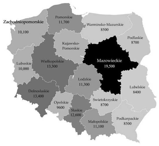 Figure 2. Regional GDP per capita (EUR, current prices, 2017), extracted from Eurostat.
 - Geographical axis: North East–South West (less developed regions except for Mazowieckie are in the north-east and most developed regions are in the west and south-west),
- Concentration of industry, including energy industry in some regions (Table 1).
 Table 1. Selected indicators for regions of Poland in 2017. Source: Data from [58].
The set of selected indicators of socio-economic development for 2017 is presented in Table 1. The data was extracted from the Local Data Bank run by Statistics Poland [58].
The central region generates almost 20% of the sold production of industry, and there are two other regions with more than 10% share. Electricity production is even more concentrated: The Dolnoslaskie region produces over 38% of the total production of electricity and two other regions have more than 15% share. These two characteristics—concentration of industry and of electricity production very significantly influence the variations in energy and emission intensity of regional economies. Official statistical data on regional GHG emissions were made available only in 2019 and covered the years 2016 and 2017. Such dataset does not allow valid temporal analysis, therefore, spatial variation in 2017 was analysed.
Key indicators related to carbon intensity and influencing factors are shown in Table 2. All indicators were own calculations except for GDP per capita. Source data on population and GDP was extracted from databases kept by the Statistics Poland [58]. Data on total regional GHG emissions were estimates by the National Centre for Emissions Management. Greenhouse gasses emission covers carbon dioxide, methane and nitrous oxide emission, excluding land use, land-use change and forestry (LULUCF). Emission was expressed in CO2 equivalent (CO2 eq).
Table 2.
Indicators related to greenhouse gases (GHG) emission intensity across Polish regions in 2017. Source: Data from [58] and own calculation.
The concentration of industry, including power industry was manifested by the fact there were 4 regions where emission per capita was higher than the national mean by more than 40% (Lodzkie—+108%, Opolskie +82%, Slaskie +45% and Swietokrzyskie +41%). However, the above-mentioned data was estimated using a production-based approach and since some industries are concentrated, they do not fully reflect the differences in emission intensity of regional economies. Additionally, the available data on regional fuels and energy consumption was not consistent with the estimates of GHG emission discussed earlier. There was also a lack of regional break-down of CO2 emissions into sectors.
Due to these constraints, detailed analysis was done for households only, using own estimates of regional energy use and CO2 emissions based on statistical data on regional fuels consumption, excluding fuels for vehicles. Calorific values and emissivity factors for CO2 were adopted according to the estimates by the National Centre for Emissions Management [59]. These estimates were used for reporting from systems covered by the Emission Trading Scheme. For electricity, CO2 emission intensity factor for the national power system was applied [60]. A similar approach was used for heat [61]. The values of respective indicators used for calculations are shown in Table 3.
Table 3.
Indicators used for estimation of energy use and CO2 emissions. Source: Data from [59,60,61].
Emission from households covered direct consumption of fuels in households (excluding fuels for vehicles), consumption of electricity and heat. Compared to total GHG emission, CO2 emission from households accounts for about 18% of domestic emission. Emission-related indicators for households based on own estimates of GHG emission for this sector are shown in Table 4.
Table 4.
Indicators related to CO2 emission intensity in households in 2017. Source: Own calculation.
Average carbon emission per capita from households decreased in Poland by 4.5% in 2017 compared to 2006. However, there were 3 regions (Dolnoslaskie, Malopolskie and Mazowieckie), where emission per capita increased. On average, the period 2006–2017 witnessed a substantial increase in disposable income of households—by almost 73%, a slight decrease in energy emissivity by 0.14% and decrease in energy intensity of consumption by 30%. Again, contrary to the general trend of improving energy efficiency and decreasing emission intensity, some regions showed deteriorating indicators. The emission factor (energy emissivity) increased in Podkarpackie, Swietokrzyskie, Wielkopolskie and Zachodniopomorskie regions. Energy intensity of consumption (measured by the relation between energy consumption and gross disposable income) decreased in all regions, ranging from 27% to almost 35%. Emissions per capita from households across regions were far less varied than the total emission per capita, although differences still exist. Total differences in CO2 emission per capita from households between regions and national average were also less varied in 2017 than in 2006 (Figure 3).
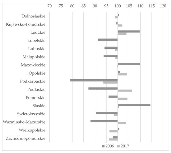
Figure 3.
Total difference in CO2 emission per capita in regions of Poland compared to the average (Poland = 100). Source: Own calculation.
The situation of the less developed regions changed substantially. In 2006, carbon emissions per capita in Podkarpackie, Podlaskie and Warminsko-Mazurskie were more than 10% below the national average. In 2017 two of them—Podlaskie and Warminsko-Mazurskie—had carbon emission per capita from households 6.2% and 3.5% above the national average, accordingly.
The differences in emission per capita were a direct result of energy use per capita and its structure by type of fuel (Figure 4).
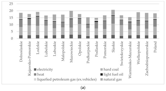
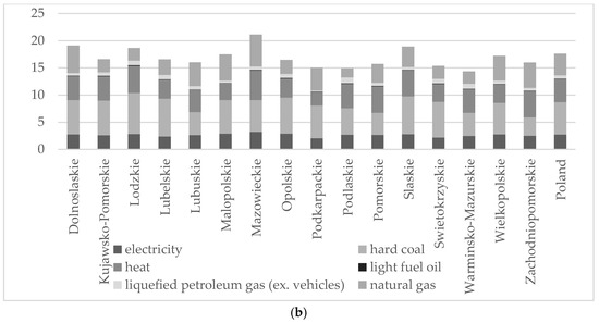
Figure 4.
Energy use in households per capita by fuels in 2006 (a) and 2017 (b) [GJ/person]. Source: Own calculation.
Energy use per capita was significantly higher in 4 regions—Mazowieckie, Dolnoslaskie, Slaskie and Lodzkie, which were also the regions with the highest GDI per capita. Differences in the level and structure of energy use per capita should be analysed in the context of diverse climate conditions and diverse needs for heating and cooling in residential buildings. Surprisingly, there was no visible increase in energy use in regions with a cooler climate (Podlaskie, Warminsko-Mazurskie). Regions of Poland were also significantly diversified in terms of urbanization and availability of district heating: Mountain regions have a smaller share of heat because heating networks are less developed there. In the next part of the paper, these differences will be investigated using decomposition analysis.
3.2. Index Decomposition Analysis Methodology
For the purpose of decomposition analysis, variables were defined according to the Kaya identity approach [62]: C—emission of greenhouse gases (carbon dioxide), E—energy consumption, Y—income, P—population. Considering the goal of this study, i.e., inter-regional comparisons, carbon emission per capita was analysed. The basic equation expresses emission per capita C’ as follows:
where C/E is aggregate emissivity of energy production, E/Y—aggregate energy intensity of GDP, Y/P—GDP per capita. This general formula was modified according to the level of analysis and limitations concerning available data.
For a general comparison between regions a simplified formula (2) was used to decompose difference in GHG emission per capita between a region i (C’Ri) and the average emission per capita:
where Ci is total greenhouse gases emission in a region i, Ci/Yi—the GHG intensity of a region’s i Gross Domestic Product and Yi/Pi—regional GDP per capita. This formula was applied because of the lack of regional energy balances that would be consistent with available GHG emission estimates.
Decomposition for households was performed using the basic formula (1) adjusted for an income indicator. Carbon intensity for households (C’H) in a region i was defined as carbon emission in households per capita. Disposable Income (DI) per capita was applied as a measure of income (Equation (3)):
Carbon emission per capita in households (C’H) was then analysed in terms of spatial differences. A detailed decomposition was done using the method of multiplicative decomposition analysis presented by Ang and Choi [63], discussed further by Ang et al. [14] and applied by Liu et al. [33], among others. Comparisons were done using a multi-regional approach, as discussed by Su and Ang [18]. In this case, with 16 regions of the same country under analysis, it was justified to take the country average (which is a group average here) as a reference value.
The differences between a region i and the respective national average (DRi) in carbon intensity and contributing indicators (denoted here generally as V) for each region were calculated as Vi/VA (total and for households). For the multiplicative decomposition, the following is true (for total carbon intensity and for households):
where Dvj represents the difference in the factor Vj between the region i and the national average and m denotes the number of factors.
Next, the decomposition was performed to calculate the contributions of each factor to the differences between the regional and national carbon intensity for each level of analysis (total and households). For weighting, the LMDI-I technique was applied (first proposed by Choi and Ang [64], Equation (6) according to the instructions by Ang [14]). This technique was recommended for intensity indicators and changes (differences) expressed in a multiplicative form. After logarithmisation, the equation takes the form (5):
making it possible to calculate the contribution Z of the factor Vj in the region i as follows (6):
4. Results
4.1. Decomposition of Differences in Total GHG Emission per Capita
Results of decomposition of the difference in GHG total emission per capita in regions of Poland compared to the average are shown in Table 5.
Table 5.
Contribution of factors to the total difference in GHG emission per capita [percentage points]. Source: Own calculation.
Based on the results, four types of regions can be distinguished according to the direction of impact of the two contributing factors. Regions where higher GDP per capita caused a rise in GHG emission per capita and GDP emission intensity contributes to lowering of this indicator (H-L), were those with the relatively high level of economic activity and resulting high GDP per capita. However, this economic activity was relatively energy-efficient and, therefore, relatively low-emission-intensive. In all regions belonging to this cluster (Dolnoslaskie, Mazowieckie, Wielkopolskie), the total emission per capita was lower than the average.
The second type (one region only) are regions with both factors contributing positively to the emission per capita higher than the average (H-H). In the Slaskie region, GHG emission per capita was higher than the average by 45.6%, of which 19.0% was the contribution of GDP per capita and 26.6% was the contribution of emission intensity of GDP. In this case, the relatively intensive economic activity was, at the same time, relatively carbon-intensive. It means that policy should be, to a large extent, targeted at lowering emission intensity and improving energy efficiency.
The third group were regions with a negative contribution of GDP per capita and positive contribution of emission intensity of GDP (L-H). Within this group, the regions where the total emission per capita was substantially higher than the national average face the biggest challenges. This means that the concentration of carbon-intensive sectors was not compensated by the adequate economic effect in terms of GDP. There were three regions of this type (L-H with emission per capita higher than the average)—Lodzkie, Opolskie and Swietokrzyskie. In these regions, the policy is more challenging as it should be directed at both economic and carbon dimensions of efficiency of the regional economy. The second sub-group was formed by regions with the total emission per capita lower than the average. In those regions (Kujawsko-Pomorskie, Lubelskie, Podlaskie, Zachodniopomorskie), the negative impact of higher carbon intensity was quite small, mainly due to the low share of carbon-intensive sectors. Development policy in these regions should promote economic activity without increasing carbon intensity, meaning that it should be selective and cautious.
The fourth group were regions with a negative contribution of GDP per capita and the negative contribution of emission intensity of GDP (L-L). These regions have less carbon-intensive economies but are also underdeveloped. The main challenge for development policy is therefore to promote a more efficient economic structure in terms of GDP rather than emission intensity itself. It can be assumed that current technological trends will act independently and contribute to the improvement of carbon efficiency.
4.2. Decomposition of Differences in CO2 Emission per Capita in Households
Results of decomposition of the difference in CO2 emission per capita in regions of Poland compared to the average are shown in Table 6 and Table 7.
Table 6.
Contribution of factors to the difference in CO2 emission per capita in households in 2006 capita [percentage points]. Source: Own calculation.
Table 7.
Contribution of factors to the difference in CO2 emission per capita in households in 2017 [percentage points]. Source: Own calculation.
The analysis shows that the main factor influencing regional differences in carbon emission per capita from households was the disposable income per capita and the resulting consumption level. In all regions except for Zachodniopomorskie, the contribution of this factor had the same direction in 2017 as in 2006, and the variation of this contribution was the largest among all three factors under analysis. This was related to the continuing pattern of regional diversification of economic development and increasing income gap between more and less developed regions (Figure 5).
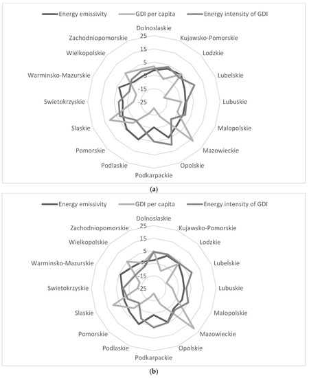
Figure 5.
Contribution of factors to the difference in regional CO2 emission per capita in 2006 (a) and 2017 (b) [percentage points]. Source: Own calculation.
Moreover, changes in the structure of energy supply, as well as the resulting changes in emission factor (energy emissivity), were far less dynamic than economic development. This was the main difference between the sector of households and the regional economies as a whole. Unlike the variation in overall emission per capita, the emissivity of energy and energy intensity of consumption in the household’s sector had a much smaller impact, and this impact was significantly less diverse.
5. Discussion
The analysis shows that the regional variation of greenhouse gas emissions per capita has a significantly different pattern in the case of total emissions than in the household sector. The regional variation of total emissions is mainly influenced by the concentration of industry, including the energy sector as well as the level of economic activity measured by GDP per capita. In the case of spatial studies at the regional level, total emissions allocated using the production approach can be misleading and should be extended by sectoral analysis and consumption-based approach, like studies on household carbon footprint [65,66]. In most countries, there is a concentration of energy-intensive and high-emission sectors in some regions. As a result, GHG emission per capita is higher than in regions with a lower share of such sectors. Such regions generate emissions “on behalf of” other regions and their emissions should be in fact allocated to other regions according to the consumption approach. In the case of total emission in regions, temporal analysis would be a more appropriate approach, and such approach was used in the majority of studies concerning regional dimensions of GHG emissions [20,33,39]. However, for Poland, such analyses are impossible because of the lack of data across sufficiently long time periods. Despite this obstacle, decomposition analysis of even one-year data can provide valuable insights concerning emission reduction policies, adjusting them in accordance to the factors dominating in particular region.
There is no problem with the concentration of industry in the case of households. The study showed that in this sector disposable income per capita is a key factor of differences in CO2 emission per capita between regions. Higher households’ incomes contribute to higher emission per capita, mostly due to the shift in consumption towards more energy- and material-intensive goods, although this impact is stronger in fast developing countries, such as China [67]. This impact is also highly differentiated across regions. Similar results were obtained in a number of other studies using different methods for different countries [66,68]. This is in line with the conclusions presented by e.g., Ottelin et al., whose analysis of consumption-based carbon footprints in 25 EU countries showed that there is a significant difference between the less developed Eastern European countries and the rest of Europe [65]. In Eastern Europe, including Poland, carbon intensities increase clearly with the increasing degree of urbanisation. In some Western European countries, such as France and Belgium, carbon footprints visibly decrease with the increasing degree of urbanisation, even after income is controlled. Interesting conclusions are drawn from the study of Jones and Kammen who, based on a broad microdata panel for the United States showed that, unlike some previous research, a negative correlation between population density (i.e., urbanization) and emissions is limited: High population density contributes to relatively low household carbon footprint in the central cities of large metropolitan areas, but extensive suburbanization in these regions contributes to an overall net increase in carbon footprint compared to smaller urban areas [69].
In this context, it is interesting how the patterns of spatial differences in Poland will change in future and whether further economic growth will affect them. This is also one of the most important recommendations for further research on household GHG emissions, especially in Poland: Research should concern different levels of spatial aggregation, including microdata.
The impact of energy emissivity is quite low and not as varied as in the case of income. This means, for example, that policies oriented around consumption of fuels can be rather uniform across regions, while more developed regions should also be subject to measures supporting less energy-intensive consumption.
It should be noted, that due to the type and scope of household emissions data used in this study only general comparisons are possible. This study is based on aggregate data and covers direct emissions related to fuels consumed by households, as well as indirect emissions related to electricity and heat consumption in households. Therefore, it is not possible to directly refer to the results of studies based on micro-data. Analyses of regional diversity of household carbon intensity should be in case of Poland complemented by sub-regional and local data, to facilitate decision making and tailoring actions at different management levels.
Systematic studies on regional carbon emissions are in Poland difficult due to data availability. Statistical data on regional GHG emission for Poland (using production approach) are presented for two years only (2016–2017), which makes it impossible to analyse long-term emission trends. Therefore, spatial-temporal analysis was not possible within this study. In particular, trajectories of changes in carbon intensity of regional economies and their causes should be investigated in future.
Despite existing gaps and limitations, this study shows that decomposition analysis is a useful tool for explaining spatial differences in greenhouse gases emissions. More in-depth knowledge about spatial dimension has also important policy-making implications: With substantial inter-regional differences, policies cannot be uniform.
Funding
This research was funded by the Ministry of Science and Higher Education of the Republic of Poland: Funds awarded to the University of Bialystok, Faculty of Economics and Finance.
Conflicts of Interest
The author declares no conflict of interest.
References
- A Policy Framework for Climate and Energy in the Period from 2020 to 2030. Communication from the Commission to the European Parliament, the Council, the European Economic and Social Committee and the Committee of Regions, COM/2014/015 Final. Available online: https://eur-lex.europa.eu/legal-content/EN/TXT/?uri=CELEX:52014DC0015 (accessed on 24 May 2020).
- EU Cohesion Policy 2014–2020, Targeting Investments on Key Growth Priorities. Available online: https://ec.europa.eu/regional_policy/sources/docgener/informat/2014/fiche_low_carbon_en.pdf (accessed on 30 August 2019).
- Proposal for a Regulation of the European Parliament and of the Council on the European Regional Development Fund and on the Cohesion Fund, COM/2018/372 Final. Available online: https://eur-lex.europa.eu/legal-content/EN/TXT/?uri=COM%3A2018%3A372%3AFIN (accessed on 24 May 2020).
- Proposal for a Regulation of the European Parliament and of the Council establishing the Just Transition Fund, COM/2020/22 Final. Available online: https://eur-lex.europa.eu/legal-content/EN/TXT/?uri=CELEX%3A52020PC0022 (accessed on 24 May 2020).
- Updated Draft Energy Policy of Poland until 2040. Available online: https://www.gov.pl/web/aktywa-panstwowe/zaktualizowany-projekt-polityki-energetycznej-polski-do-2040-r (accessed on 24 May 2020).
- Resolution of the Council of Ministers of 16 July 2019 on the State Environmental Policy 2030 (Uchwała nr 67 Rady Ministrów z dnia 16 lipca 2019 r. w Sprawie Przyjęcia “Polityki Ekologicznej Państwa 2030—Strategii Rozwoju w Obszarze środowiska i Gospodarki Wodnej). Available online: http://prawo.sejm.gov.pl/isap.nsf/DocDetails.xsp?id=WMP20190000794 (accessed on 24 May 2020).
- National Strategy for Regional Development (Krajowa Strategia Rozwoju Regionalnego). 2019. Available online: https://www.gov.pl/attachment/38c54257-5b35-4b2d-b379-c897a31c85e7 (accessed on 25 May 2020).
- Pearl, J. Causality; Cambridge University Press: Cambridge, UK, 2009; ISBN 978-0-521-89560-6. [Google Scholar]
- Ang, B.W.; Liu, N. Energy decomposition analysis: IEA model versus other methods. Energy Policy 2007, 35, 1426–1432. [Google Scholar] [CrossRef]
- Ang, B.W.; Goh, T. Index decomposition analysis for comparing emission scenarios: Applications and challenges. Energy Econ. 2019, 83, 74–87. [Google Scholar] [CrossRef]
- Su, B.; Ang, B.W. Structural decomposition analysis applied to energy and emissions: Some methodological developments. Energy Econ. 2012, 34, 177–188. [Google Scholar] [CrossRef]
- Hoekstra, R.; van den Bergh, J.C.J.M. Comparing structural decomposition analysis and index. Energy Econ. 2003, 25, 39–64. [Google Scholar] [CrossRef]
- Sun, J.W. Changes in energy consumption and energy intensity: A complete decomposition model. Energy Econ. 1998, 20, 85–100. [Google Scholar] [CrossRef]
- Ang, B.W. LMDI decomposition approach: A guide for implementation. Energy Policy 2015, 86, 233–238. [Google Scholar] [CrossRef]
- Ang, B.W. Decomposition analysis for policymaking in energy: Which is the preferred method? Energy Policy 2004, 32, 1131–1139. [Google Scholar] [CrossRef]
- Soytaş, U.; Sarı, R. Routledge Handbook of Energy Economics; Routledge: Abington, UK, 2019; ISBN 978-1-315-45963-9. [Google Scholar]
- Choi, K.-H.; Ang, B.W. Attribution of changes in Divisia real energy intensity index—An extension to index decomposition analysis. Energy Econ. 2012, 34, 171–176. [Google Scholar] [CrossRef]
- Su, B.; Ang, B.W. Multi-region comparisons of emission performance: The structural decomposition analysis approach. Ecol. Indic. 2016, 67, 78–87. [Google Scholar] [CrossRef]
- Ang, B.W.; Xu, X.Y.; Su, B. Multi-country comparisons of energy performance: The index decomposition analysis approach. Energy Econ. 2015, 47, 68–76. [Google Scholar] [CrossRef]
- Song, C.; Zhao, T.; Wang, J. Spatial-temporal analysis of China’s regional carbon intensity based on ST-IDA from 2000 to 2015. J. Clean. Prod. 2019, 238, 117874. [Google Scholar] [CrossRef]
- Zhang, W.; Li, K.; Zhou, D.; Zhang, W.; Gao, H. Decomposition of intensity of energy-related CO2 emission in Chinese provinces using the LMDI method. Energy Policy 2016, 92, 369–381. [Google Scholar] [CrossRef]
- Zhang, C.; Wu, Y.; Yu, Y. Spatial decomposition analysis of water intensity in China. Socioecon. Plann. Sci. 2020, 69, 100680. [Google Scholar] [CrossRef]
- Huang, J.; Du, D.; Tao, Q. An analysis of technological factors and energy intensity in China. Energy Policy 2017, 109, 1–9. [Google Scholar] [CrossRef]
- Zhao, X.; Zhang, Y.; Li, Y. The spillovers of foreign direct investment and the convergence of energy intensity. J. Clean. Prod. 2019, 206, 611–621. [Google Scholar] [CrossRef]
- Yan, H. Provincial energy intensity in China: The role of urbanization. Energy Policy 2015, 86, 635–650. [Google Scholar] [CrossRef]
- Aldieri, L.; Kotsemir, M.; Paolo Vinci, C. Environmental innovations and productivity: Empirical evidence from Russian regions. Resour. Policy 2019, in press. [Google Scholar] [CrossRef]
- Bossanyi, E. UK primary energy consumption and the changing structure of final demand. Energy Policy 1979, 7, 253–258. [Google Scholar] [CrossRef]
- Ang, B.W.; Zhang, F.Q. A survey of index decomposition analysis in energy and environmental studies. Energy 2000, 25, 1149–1176. [Google Scholar] [CrossRef]
- Xu, X.Y.; Ang, B.W. Index decomposition analysis applied to CO2 emission studies. Ecol. Econ. 2013, 93, 313–329. [Google Scholar] [CrossRef]
- Ang, B.W.; Zhang, F.Q. Inter-regional comparisons of energy-related CO2 emissions using the decomposition technique. Energy 1999, 24, 297–305. [Google Scholar] [CrossRef]
- Kim, K.; Kim, Y. International comparison of industrial CO2 emission trends and the energy efficiency paradox utilizing production-based decomposition. Energy Econ. 2012, 34, 1724–1741. [Google Scholar] [CrossRef]
- Fernández González, P.; Landajo, M.; Presno, M.J. Multilevel LMDI decomposition of changes in aggregate energy consumption. A cross country analysis in the EU-27. Energy Policy 2014, 68, 576–584. [Google Scholar] [CrossRef]
- Liu, N.; Ma, Z.; Kang, J. A regional analysis of carbon intensities of electricity generation in China. Energy Econ. 2017, 67, 268–277. [Google Scholar] [CrossRef]
- Hang, Y.; Wang, Q.; Wang, Y.; Su, B.; Zhou, D. Industrial SO2 emissions treatment in China: A temporal-spatial whole process decomposition analysis. J. Environ. Manag. 2019, 243, 419–434. [Google Scholar] [CrossRef]
- Shi, Z.; Huang, H.; Wu, F.; Chiu, Y.; Zhang, C. The Driving Effect of Spatial Differences of Water Intensity in China. Nat. Resour. Res. 2019, 1–14. [Google Scholar] [CrossRef]
- Yao, L.; Zhang, H.; Zhang, C.; Zhang, W. Driving effects of spatial differences of water consumption based on LMDI model construction and data description. Clust. Comput. 2019, 22, 6315–6334. [Google Scholar] [CrossRef]
- Wang, Y.; Yang, G.; Dong, Y.; Cheng, Y.; Shang, P. The Scale, Structure and Influencing Factors of Total Carbon Emissions from Households in 30 Provinces of China—Based on the Extended STIRPAT Model. Energies 2018, 11, 1125. [Google Scholar] [CrossRef]
- Shi, Y.; Han, B.; Han, L.; Wei, Z. Uncovering the national and regional household carbon emissions in China using temporal and spatial decomposition analysis models. J. Clean. Prod. 2019, 232, 966–979. [Google Scholar] [CrossRef]
- Zhang, P.; Duan, M.; Yin, G. The Periodic Characteristics of China’s Economic Carbon Intensity Change and the Impacts of Economic Transformation. Energies 2018, 11, 961. [Google Scholar] [CrossRef]
- Lin, J.; Liu, Y.; Hu, Y.; Cui, S.; Zhao, S. Factor decomposition of Chinese GHG emission intensity based on the Logarithmic Mean Divisia Index method. Carbon Manag. 2014, 5, 579–586. [Google Scholar] [CrossRef]
- Xu, X.; Tan, Y.; Chen, S.; Yang, G.; Su, W. Urban Household Carbon Emission and Contributing Factors in the Yangtze River Delta, China. PLoS ONE 2015, 10, e0121604. [Google Scholar] [CrossRef] [PubMed]
- Ahmad, S.; Baiocchi, G.; Creutzig, F. CO2 Emissions from Direct Energy Use of Urban Households in India. Environ. Sci. Technol. 2015, 49, 11312–11320. [Google Scholar] [CrossRef] [PubMed]
- Hargreaves, K.; Preston, I.; White, V.; Thumim, J. The distribution of household CO2 emissions in Great Britain. JRF Programme Pap. Clim. Chang. Soc. Justice Updat. Version Suppl. Proj. Pap. 2013, 1, 1998–2004. [Google Scholar]
- Andrés, L.; Padilla, E. Energy intensity in road freight transport of heavy goods vehicles in Spain. Energy Policy 2015, 85, 309–321. [Google Scholar] [CrossRef]
- Fernández González, P.; Landajo, M.; Presno, M.J. The Divisia real energy intensity indices: Evolution and attribution of percent changes in 20 European countries from 1995 to 2010. Energy 2013, 58, 340–349. [Google Scholar] [CrossRef]
- Fernández González, P. Exploring energy efficiency in several European countries. An attribution analysis of the Divisia structural change index. Appl. Energy 2015, 137, 364–374. [Google Scholar] [CrossRef]
- Fernández González, P.; Presno, M.J.; Landajo, M. Regional and sectoral attribution to percentage changes in the European Divisia carbonization index. Renew. Sustain. Energy Rev. 2015, 52, 1437–1452. [Google Scholar] [CrossRef]
- Fernández González, P.; Landajo, M.; Presno, M.J. The Driving Forces of Change in Environmental Indicators; Lecture Notes in Energy; Springer International Publishing: Cham, Switzerland, 2014; Volume 25, ISBN 978-3-319-07505-1. [Google Scholar]
- Barrett, J.; Wiedmann, T.; Minx, J. Understanding Changes in UK CO2 Emissions 1992–2004: A Structural Decomposition Analysis; Report to the UK Department for Environment, Food and Rural Affairs; Stockholm Environment Institute and Durham Business School, 2009; Available online: https://www.sei.org/mediamanager/documents/Publications/SEI-ResearchReport-Minx-UnderstandingChangesInUKCO2Emissions-1992-2004-AStructuralDecompositionApproach-2009.pdf (accessed on 25 February 2020).
- Hammond, G.P.; Norman, J.B. Decomposition analysis of energy-related carbon emissions from UK manufacturing. Energy 2012, 41, 220–227. [Google Scholar] [CrossRef]
- Seibel, S. Decomposition Analysis of Carbon Dioxide-Emission Changes in Germany—Conceptual Framework and Empirical Results (PDF); Office for Official Publications of the European Communities: Luxembourg, 2003. [Google Scholar]
- Jensen, P.R.; Olsen, T. Analysis of Changes in Air Emissions in Denmark; Statistics Denmark: Copenhagen, Denmark, 2003. [Google Scholar]
- van Megen, B.; Bürer, M.; Patel, M.K. Comparing electricity consumption trends: A multilevel index decomposition analysis of the Genevan and Swiss economy. Energy Econ. 2019, 83, 1–25. [Google Scholar] [CrossRef]
- Ivanova, D.; Vita, G.; Steen-Olsen, K.; Stadler, K.; Melo, P.C.; Wood, R.; Hertwich, E.G. Mapping the carbon footprint of EU regions. Environ. Res. Lett. 2017, 12, 54013. [Google Scholar] [CrossRef]
- Gozdek, A.; Szaruga, E. Analiza dekompozycyjna wzrostu emisji gazów cieplarnianych z transportu samochodowego na przykładzie Polski i Rumunii. Zesz. Naukowe. Probl. Transp. Logist. Uniw. Szczec. 2015, 29, 371–383. [Google Scholar] [CrossRef]
- Iskrzycki, K.; Suwała, W.; Kaszyński, P. Dekompozycja redukcji emisji dwutlenku siarki w polskich elektrowniach, 1995–2008. Polityka Energ. 2011, 14, 107–125. [Google Scholar]
- Suwała, W. Perspektywy technologii węglowych w energetyce w warunkach ograniczenia emisji dwutlenku węgla/Prospects of coal based power in the carbon emissions limiting system. Polityka Energ. 2008, 11, 489–497. [Google Scholar]
- Statistics Poland—Local Data Bank. Available online: https://bdl.stat.gov.pl/BDL/dane/podgrup/temat (accessed on 7 March 2020).
- Wartości Opałowe (WO) i Wskaźniki Emisji CO2 (WE) w roku 2017 do Raportowania w Ramach Systemu Handlu Uprawnieniami do Emisji za rok 2020 (Calorific Values and Emission Factors in 2017 for Reporting within the Emissions Trading Scheme in 2020); Krajowy Ośrodek Bilansowania i Zarządzania Emisjami/The National Centre for Emissions Management: Warsaw, Poland, 2019; Available online: https://www.kobize.pl/uploads/materialy/download/WO_i_WE_do_monitorowania-ETS-2020.pdf (accessed on 10 February 2020).
- Wskaźniki Emisyjności CO2, SO2, NOx, CO i pyłu Całkowitego dla Energii Elektrycznej na Podstawie Informacji Zawartych w Krajowej bazie o Emisjach Gazów Cieplarnianych i Innych Substancji za 2017 rok (Emission Factors for CO2, SO2, NOx, CO and Dust for Electricity, According to National Base on Emissions of Greenhouse Gases, 2017); Krajowy Ośrodek Bilansowania i Zarządzania Emisjami/The National Centre for Emissions Management: Warsaw, Poland, 2018; Available online: https://www.kobize.pl/uploads/materialy/materialy_do_pobrania/wskazniki_emisyjnosci/Wskazniki_emisyjnosci_grudzien_2019.pdf (accessed on 10 February 2020).
- Energetyka Cieplna w Liczbach 2018 (Heat Sector in Numbers 2018, Document in Polish); Urząd Regulacji Energetyki/Energy Regulatory Office: Warsaw, Poland, 2018. Available online: https://www.ure.gov.pl/download/9/10380/Energetykacieplnawliczbach-2018.pdf (accessed on 11 February 2020).
- Environment, Energy, and Economy: Strategies for Sustainability; Kaya, Y., Yokobori, K., Eds.; United Nations University Press: Tokyo, Japan, 1997. [Google Scholar]
- Ang, B.W.; Choi, K.-H. Decomposition of Aggregate Energy and Gas Emission Intensities for Industry: A Refined Divisia Index Method. Energy J. 1997, 18, 59–73. [Google Scholar] [CrossRef]
- Choi, K.-H.; Ang, B.W. Decomposition of aggregate energy intensity changes in two measures: Ratio and difference. Energy Econ. 2003, 25, 615–624. [Google Scholar] [CrossRef]
- Ottelin, J.; Heinonen, J.; Nässén, J.; Junnila, S. Household carbon footprint patterns by the degree of urbanisation in Europe. Environ. Res. Lett. 2019, 14, 114016. [Google Scholar] [CrossRef]
- Druckman, A.; Jackson, T. The carbon footprint of UK households 1990–2004: A socio-economically disaggregated, quasi-multi-regional input–output model. Ecol. Econ. 2009, 68, 2066–2077. [Google Scholar] [CrossRef]
- Zhang, H.; Lahr, M.L.; Bi, J. Challenges of green consumption in China: A household energy use perspective. Econ. Syst. Res. 2016, 28, 183–201. [Google Scholar] [CrossRef]
- Wang, C.; Guo, Y.; Shao, S.; Fan, M.; Chen, S. Regional carbon imbalance within China: An application of the Kaya-Zenga index. J. Environ. Manag. 2020, 262, 110378. [Google Scholar] [CrossRef]
- Jones, C.; Kammen, D.M. Spatial Distribution of U.S. Household Carbon Footprints Reveals Suburbanization Undermines Greenhouse Gas Benefits of Urban Population Density. Environ. Sci. Technol. 2014, 48, 895–902. [Google Scholar] [CrossRef] [PubMed]


© 2020 by the author. Licensee MDPI, Basel, Switzerland. This article is an open access article distributed under the terms and conditions of the Creative Commons Attribution (CC BY) license (http://creativecommons.org/licenses/by/4.0/).