1. Introduction
Smart meters make it possible to capture building power consumption at fine-grained temporal resolutions. Combined with analytics algorithms to extract knowledge from the raw data, many details about operative electrical appliances can be extracted. The employed algorithms, commonly referred to as Non-Intrusive Load Monitoring (NILM) methods [
1], essentially work as follows. They monitor a building’s aggregate power demand for characteristic consumption patterns to ultimately determine what appliances were operated, and when. Collecting data from a single sensing location (the smart meter) provides a cost-effective method to attribute energy consumption to individual devices [
2,
3]. The accuracy of the load identification process is, however, tightly coupled to the information content of the data available for analysis. In fact, NILM algorithms often yield mediocre results when the input data resolution is too low [
4].
A distinction between two fundamental types of electrical load signatures, differentiated by their sampling frequencies, has thus been proposed in [
5].
Microscopic load signatures are sampled at frequencies much greater than the frequency of the AC mains, and thus inherently reflect the characteristics of the (largely recurrent) voltage and current waveforms. They enable the identification of appliances and their modes of operation at a high level of accuracy, and even create the foundation for more extensive data analysis. However, such high sampling rates pose challenges to data transmission and storage, particularly when the communication channel only features a limited bandwidth [
6,
7]. In turn,
macroscopic load signatures are reported at rates lower than the nominal mains frequency, such as once per second. As waveform detail of voltage and current signals can no longer be retained at this temporal resolution, macroscopic load signatures generally only contain Root Mean Square (RMS) values of the signals, computed across one or multiple mains periods. This greatly reduces the requirements for data storage and transmission, while still permitting some NILM techniques to be applied, e.g., to infer the operating status and nature of the devices [
8,
9,
10]. Several research works, such as [
11,
12,
13,
14], have studied the analysis of microscopic load signatures in the context of NILM. They have unambiguously arrived at the fundamental insight that there is a relationship between the information content of the load the signatures and the sampling frequency at which these signatures have been gathered. Simply put, greater sampling rates have been determined to lead to a greater information content in load signature data [
15,
16,
17]. Microscopic data thus bear a great promise for the realization of accurate NILM solutions.
The ensuing high data rates of microscopic data necessitate powerful computer systems for their processing. Current NILM algorithms are thus mostly executed on powerful hosts or even in cloud computing environments in order to cope with the prevailing data rates. The option to pre-process microscopic data locally on the smart meter, in order to extract features of relevance to NILM algorithms, has in contrast not been widely explored, apart from the compression of data [
18,
19]. However, virtually all power grids worldwide are based on AC power, and microscopic waveforms of electrical voltages and currents often bear a high resemblance across successive mains periods. We demonstrate that microscopic signal trajectories can often be closely approximated by parametric waveform shapes in this work. This reduces the corresponding communication overhead, as only a small number of parameters are transmitted in place of the raw data. Furthermore, dissecting appliance current data into its constituents also facilitates the identification of certain electrical appliances based on the characteristic model parameters of the waveform signatures they exhibit. Through a set of practical studies, we prove that only a few distinct waveform patterns are required to accurately approximate the current consumption data from two widely used real-world data sets.
Our manuscript is organized as follows. In
Section 2, we introduce work related to NILM and the identification of fundamental waveform shapes in microscopic load signature data. In
Section 3, we present insights from a preliminary study, which was performed to make informed decisions on the parameter choices for our system. Subsequently, the system design used to conduct our study is introduced in
Section 4. We evaluate to what extent real-world waveform data can be represented using our parameterizable models in
Section 5 and discuss the results of the experiments conducted. Lastly,
Section 6 summarizes the insights gained in our study and presents possible future work.
2. Background and Related Work
NILM is the process of determining the power consumption of individual appliances from the aggregate consumption of an entire building or building complex. By discovering the types of present appliances as well as their operational modes, many services can be realized, including the prediction of future electricity demand and the recognition of anomalous consumption patterns. The attribution of energy demand to individual appliances even makes it possible to emit recommendations for replacing energy-hungry devices by more efficient models [
20,
21]. In order to foster wide acceptance among its users, devices to facilitate load analysis must be unobtrusive (hence the name
non-intrusive load monitoring). NILM thus relies on single measurement device (generally a smart meter [
8,
22]), which satisfies this requirement. With NILM being an active field of research, a variety of approaches to accomplish good disaggregation levels have been presented. While early proposals like [
1] were predominantly based on the detection of step changes in a household’s power consumption, a trend towards the usage of more complex algorithms can be observed in practice today [
3,
21]. Most remarkably, artificial neural networks are widely being adopted to discover patterns in load signature data [
23,
24,
25]. These not only require large amounts of training data to yield good levels of disaggregation accuracy, but often also have high demands for system memory to store and update their internal representations. Embedded metering devices are rarely equipped with plentiful resources, and as a consequence virtually all current NILM algorithms are executed on computationally powerful systems. This becomes particularly important when using microscopic load signatures (like in [
11,
12,
13]) due to the much greater rate at which data are being collected: 100
[
26], 250
[
27], and even beyond [
28].
The inclusion of a data compression step for raw voltage and current samples has been shown to lead to a significantly reduced communication overhead [
18,
19,
29,
30,
31]. Eliminating redundancies from the data while leaving the characteristic features intact can even be considered as a pre-processing step for NILM applications. Both lossless and lossy data compression algorithms have been demonstrated to be applicable to load signature data [
18,
32]. The inherent noise floor introduced by voltage and current transducers, however, leads to a degraded compressibility of microscopic load signature data when using lossless algorithms. Consequently, the lossy compression of microscopic load signature data is generally accepted, as long as the errors introduced by the compression step are sufficiently small [
19,
32]. As a side effect of applying data compression, the training of NILM algorithms that leverage artificial intelligence can often be accelerated when they are provided with meaningful features instead of requiring them to autonomously identify the relevant characteristics from raw and possibly redundant input data. Pre-processing thus appears as a viable supplement to NILM, even though only a single technique,
event detection, is widely used and implemented in NILM systems today [
33,
34,
35]. The need for data compression is less pronounced when operating on macroscopic time scales (i.e., when considering the use of electrical appliances during the course of a day), given the moderate amount of data (generally less than 1 MB per day) generated. Still, extracting Partial Usage Pattern (PUPs) [
31] from raw data has emerged as a viable means to reduce their size even further, and simultaneously pre-process the data for their usage in NILM settings in which waveform data is not required for analysis.
As our main contribution of this work is the assessment to what extent microscopic waveform data can be approximated by parametric models, it shares similarities with the concept of transform coding. However, in contrast to the general-purpose waveform decomposition mechanisms like the Fast Fourier [
36] and Wavelet [
37] transforms, we follow a data-driven approach to derive the fundamental model shapes from real-world data. A similar concept is only presented in [
38], in which typical waveform components are modeled as so-called
atoms, i.e., sinusoidal waveform components which can be parameterized and superimposed to reconstruct the input data. Confining atoms to sinusoidal components, however, limits the range of waveform characteristics they can capture, given its similarity to the Fourier transform. Still, this coding technique has been determined to yield the highest compression gains when compared to other methods in [
29]. Finally, the concept of Symbolic Aggregate approXimations (SAX) [
39] has been proposed to transform input data into
symbolic approximations by reducing both their temporal and amplitude resolutions. The non-linearity of the transformation and its inherently very lossy nature, however, render it inapplicable in the scenario of load signature analysis.
Our approach to reduce microscopic load signatures to a linear combination of parameterizable waveform shapes also allows for the modeling of non-sinusoidal components. Even though this complicates their representation as a continuous function, it reduces the computational burden on the sensing systems to a simple time-series matching, instead of requiring the computation of the full atom’s trajectory for the time frame under consideration. It can thus be considered as a lossy compression scheme, which at the same time facilitates the execution of NILM algorithms by separating actual consumption waveforms into their constituents.
3. Preliminary Feasibility Study
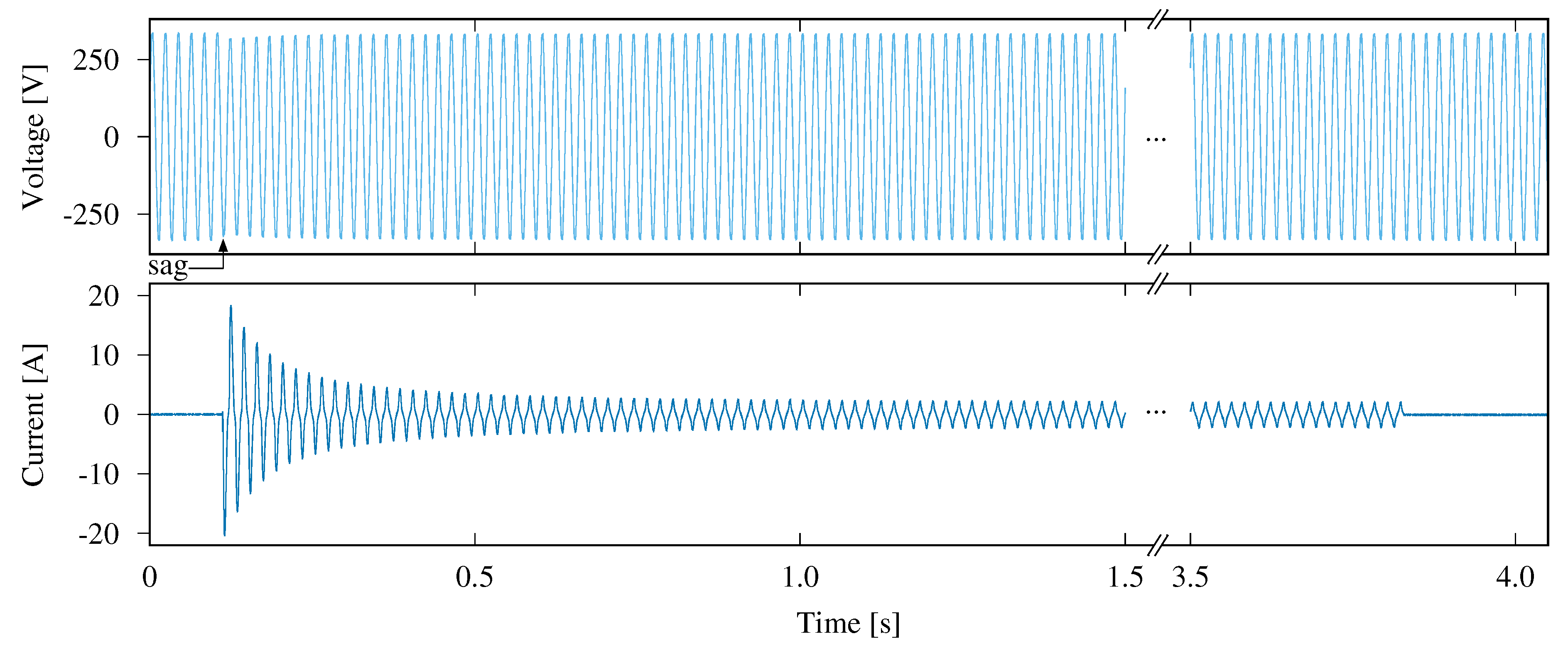
In order to establish the foundation for the contribution of this paper, let us look at the voltage and current waveforms of an electric saw appliance during the moments of its activation and deactivation, as shown in
Figure 1. The input data for this trace has been taken from the COOLL data set [
26] and was collected in Orléans, France, where the nominal mains frequency is 50
. The voltage signal, shown in the upper diagram, exhibits minimal load-dependent fluctuations: In fact, the resistance of the wiring within the building only leads to a small (but discernible) sag of the voltage signal for a few mains periods, before it returns to its nominal level. The current intake of the appliance in the lower figure, however, clearly shows a large inrush transient, followed by an exponentially declining current envelope for about
, until it converges to a steady operating current. When the electric saw is being turned off (at
in the plot), its operating current drops to zero.
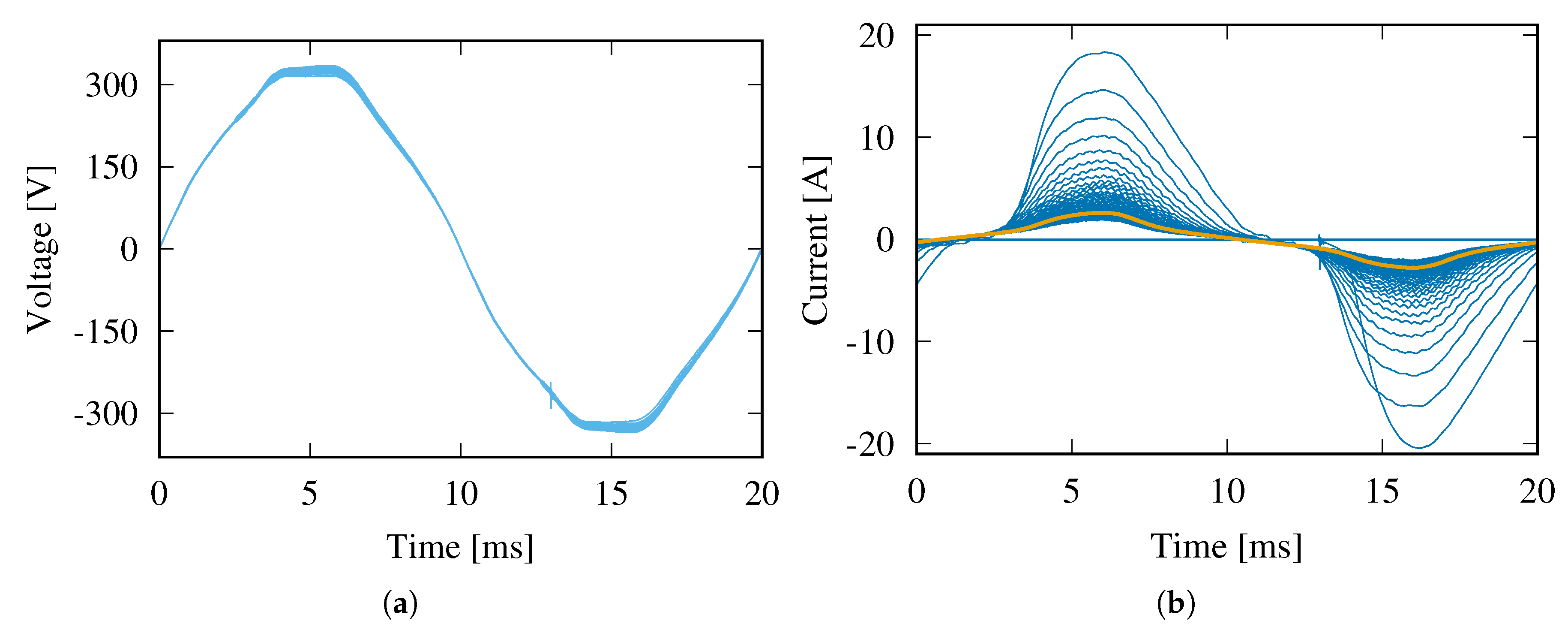
A superposition of all voltage and current waveforms experienced during the appliance operation is shown in
Figure 2. The diagram confirms that the voltage has a largely coherent waveform trajectory, revealing little if any information about the operation of the appliance. In contrast to this, the overlaid visualization of the current waveforms in
Figure 2b exhibits two major consumption levels: One at
(while the appliance was turned off), the other one at
during steady-state operation. A small number of cycles with greater current intake are only observed shortly after the activation of the device. Combined with the insights gained from
Figure 1, this motivates our choice to disregard the amplitude of the voltage channel from further analysis, and solely focus on current consumption data instead. Note that we could have equally well considered appliance power demands (with power
for voltage
V and current
I), as our proposed mechanism is applicable to any kind of input data, as long as they can be separated into cycles of equal duration.
For the electric saw appliance under consideration, let us analyze next how well a single parametric waveform shape (referred to as a
template from here on) can be used to reconstruct the complete current signal. Note that an in-depth analysis for the choice of the number of templates is presented in
Section 4.2. For our preliminary analysis, we apply the following processing steps to the waveform data:
We determine the zero-crossings of the voltage channel in order to delineate the mains periods from each other. By separating the current signal at all temporal offsets where voltage zero-crossings with a positive slope are encountered, we ensure that the resulting current waveform fragments are exactly one mains period long and their phase shift (if any) is retained.
We remove all periods with RMS currents just above the transducer noise level ( 1 ) from the data, in order to exclude data solely composed of transducer noise rather than an actual appliance operating current.
We determine the single most representative waveform from the data by using a
k-means clustering algorithm with
. This step yields the template shown as a highlighted line in
Figure 2b.
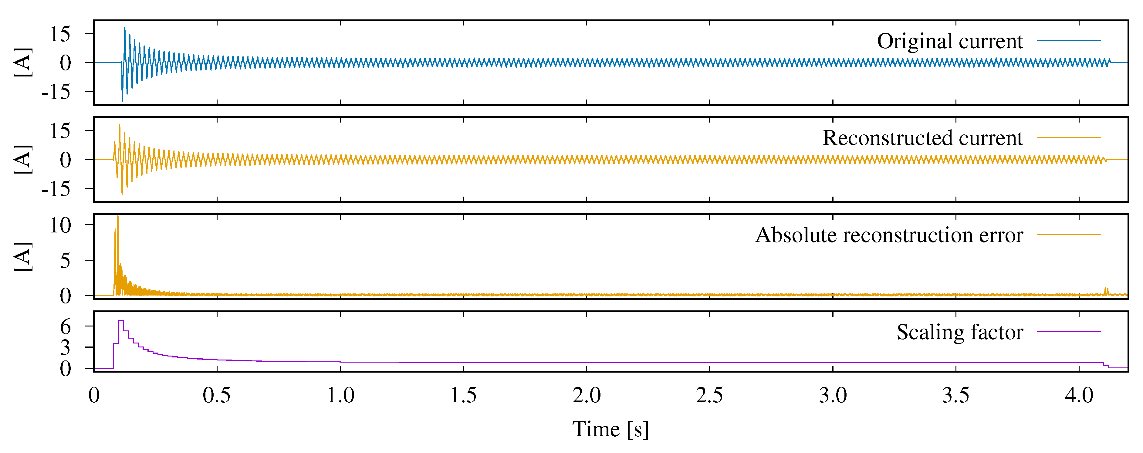
The extracted template can be parameterized in two dimensions: Amplitude (through its multiplication by a non-negative factor) and phase shift (by circular value shifting). We confine this preliminary study to the effect of amplitude scaling, and visualize the corresponding effects in
Figure 3. First, the input current waveform is analyzed in order to derive the scaling factors for each mains period, using which the difference between original data (top diagram) and the scaled template (second from the top) is minimal. The resulting scaling factors, leading to the closest approximation of the input data by the parameterized template, are given in the bottom diagram of
Figure 3; they remain fixed across each mains period. It becomes apparent that a noticeable absolute reconstruction error (third plot) can mainly be observed during the initial transient as well as when the appliance is being deactivated. The reasons therefore are twofold and explicable as follows: First, given that we have not applied any temporal shifting in our fitting step, the changing phase shift during the appliance’s activation phase (cf.
Figure 2b) cannot be correctly captured. Second, the fitting step always reconstructs full waveforms, even though the appliance activation and deactivation are not aligned with the voltage zero-crossing. The larger errors thus follow from the attempt of scaling a full template to match a partial waveform. Still, this preliminary study has shown that the discrepancies between actual and reconstructed current draw are mostly small, and that the use of parametric templates is not only viable to reduce the data resolution, but also to detect state changes. We thus continue with an in-depth investigation of the methodology to create a template library that allows for the decomposition of waveforms (collected from either a single or multiple appliances) into the underlying set of templates and their optimal parameter values.
4. Data Processing Steps and System Design
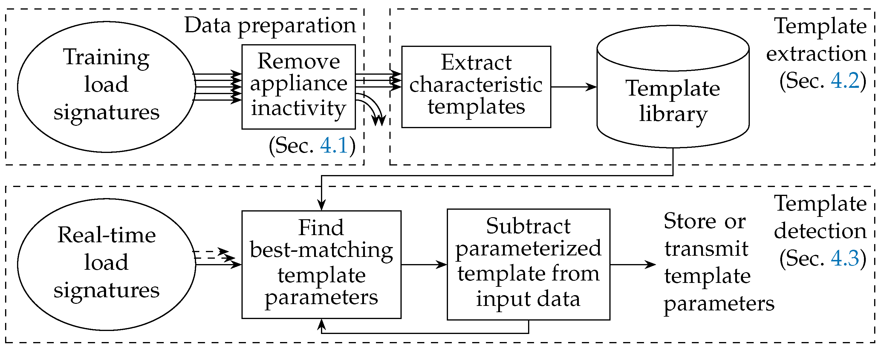
In order to study how well a set of templates is suited to approximate electrical current consumption data, we implement a system design for the processing of microscopic load signatures, according to the processing flow depicted in
Figure 4. In the upper part of the diagram, the
data preparation and
template extraction steps are shown, targeting to identify the most representative waveforms from the available input data. Once the input time series data has been separated into cycle-by-cycle data (aligned by the periods of the AC mains voltage), all mains cycles captured during appliance inactivity are removed. Next, representative templates are extracted from the remaining data, and finally stored in the
template library. We discuss the data preparation and template extraction steps in more detail in
Section 4.1 and
Section 4.2, respectively. Ideally, a large number of training load signatures is used for the template extraction step, in order to capture representative templates that model all operating modes of the appliances under consideration well.
The template library is subsequently used in the
template detection step, where real-time load signature data is approximated by the previously extracted set of parametric models. The primary objective of this step is to identify the template library entry as well as its parameter values (amplitude scaling and phase shift) to match the input data best. The fitting step is repeatedly performed until the residual difference is either very small or can no longer be modeled by any of the templates in the library. Once parameter values for all contained templates have been identified, our system condenses each mains period into one or more tuples indicating the respective template identifier as well as its amplitude scaling factor and phase shift. We discuss how template parameters are determined and how a linear combination of parameterized templates can be used to approximate appliance current consumption in
Section 4.3.
4.1. Preparing Data for the Template Extraction
Current consumption data are generally available as a sequence of values over time. In order to identify fundamental parametric waveforms, these time series data must be separated into the underlying mains voltage cycles. We proceed in the same way as described in
Section 3 and use the zero-crossings of the voltage channel in order to delineate the mains periods from each other. In the rare event when two zero-crossings are observed quick succession, we select the one that delineates the two mains cycles such that their lengths are closest to the average number of samples per mains period. As only measurements collected during an appliance’s activity can be considered for the extraction of representative templates, we disregard samples in which the RMS current ranges below 1
; a value that has been empirically determined to work across all data sets we have used. Given the importance of the template extraction step, however, an adaptation of this value to the specifics of the transducer is imperative to eliminate any readings from mains periods during which no appliances are operative.
Next, the waveform data is denoised by applying a Wavelet filter, as proposed in [
40]. This step eliminates the noise induced by the current transducer. Furthermore, we eliminate a range of errors sporadically present in existing data sets, such as singular outlier values or incorrect algebraic signs. This filtering step is important to increase the similarity of waveform data before running the template extraction step, as it facilitates the clustering process and reduces the risks of adapting to the noise characteristics too well. It is important to note, however, that denoising is only applied during the template extraction step, whereas unfiltered data are being used during the subsequent template identification (cf.
Section 4.3).
At last, the waveform data undergo a two-stage normalization stage in order to ensure their comparability. First, we normalize the amplitudes of the waveform data to the range. This ensures the comparability of waveforms, irrespective of their original amplitude. Second, we eliminate any phase shift information by applying a cyclic rotation until the waveform’s zero-crossings are aligned to the beginning, mid-point, and end of the mains period under consideration as closely as possible. This phase normalization step is required to make sure that phase-shifted, but otherwise identical, sequences can be identified as such during the template identification.
4.2. Template Identification by Clustering
Clustering is the process of finding groups of similar elements or hidden patterns in a set of input data. As our objective is to identify the fundamental waveform trajectories in electrical current consumption data, we apply a clustering step to identify the fundamental waveform templates from the large number of input waveforms that result from the data preparation described in
Section 4.1. The application of clustering generally requires three parameters to be determined:
The clustering method used to combine similar waveforms into the same cluster,
the required dis-similarity between clusters (i.e., their distance), and
the metric to compute the similarity of two elements.
While we had manually fixed the number of clusters to one in
Section 3, the number of distinct templates is much greater in practice, and generally correlated with the number and types of appliances under consideration. This number is not generally known in advance, given that new electrical appliances are being developed and brought to market constantly. As a result, only a small subset of the existing clustering algorithms is applicable for the task at hand, namely
non-parametric algorithms. We rely on the Hierarchical Agglomerative Clustering (HAC) method because it determines the number of clusters autonomously, based a configurable minimum
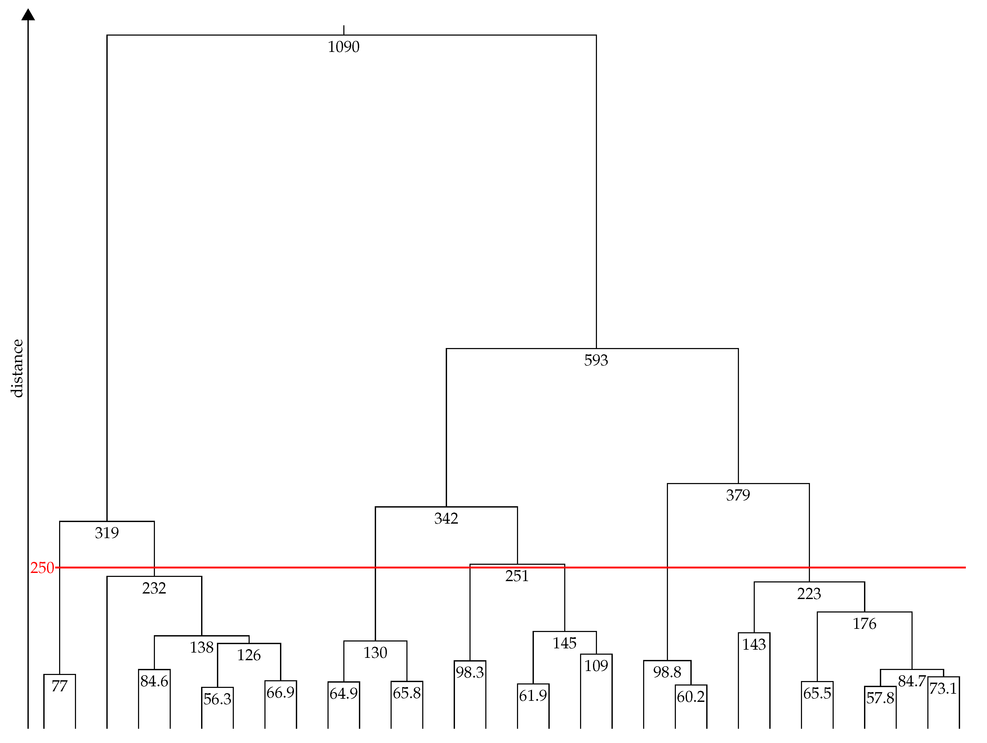
distance requirement. The greater the allowed distance of templates from each other, the smaller the number of templates. As a positive side effect that facilitates the data analysis, HAC creates a hierarchical tree of the detected clusters, which allows for a simple translation of required minimal distance to the corresponding number of output clusters, and vice versa. An example for such a tree, known as a
dendrogram, is given in Figure 6 below.
Having selected a clustering method, and thus fulfilling Item 1 of the listed requirements above, it still remains open to choose a suitable metric to quantify the similarity of two waveforms as well as a dis-similarity measurement for determined clusters. Given that multiple choices are possible for either item, we have run a comparative study for a range of candidate solutions. In our analysis, we consider five different cluster distance metrics: Weighted average linkage (WA), simple-linkage clustering (SL), complete-linkage clustering (CL), Centroid linkage clustering (CE), and Ward’s method [
41] (WM) as options for Item 2. In a similar fashion, we assess the impact of two similarity metrics for waveform data, namely their Euclidean distance (ED) and their cross-correlation (CC). As only the Euclidean distance can be used in conjunction with the Centroid linkage clustering and Ward’s method, we confine our analysis to the valid combinations. For our investigation of how the distance and similarity metrics influence the identification of the fundamental waveform trajectories, we have run a study based on the COOLL data set [
26] (see
Section 5.1 for more details). For this experiment, all current waveforms during the activities of all appliances were extracted, preprocessed as described in
Section 4.1, and clustered by means of the HAC method. Subsequently, we have assessed the achievable minimal reconstruction error by reconstructing the input data by means of the available templates (through amplitude scaling and phase shifting; cf.
Section 4.3). By calculating the Root Mean Square Error (RMSE) as a measure of the difference between the original data and their closest reconstruction, we quantify how closely the parametric templates can approximate the raw data.
The results are shown in
Figure 5, where the corresponding RMSE values are plotted against the maximum permitted number of clusters. It becomes apparent that Ward’s method consistently yields the lowest RMSE values when more than three templates are being extracted. Therefore, the combination of Ward’s method and the Euclidean distance are used throughout the remainder of this manuscript. The resulting hierarchical cluster layout when applying HAC with these metrics is shown in the dendrogram in
Figure 6. Note that the distance on the y-axis shows the Euclidean distance between two waveform trajectories, not the RMSE.
We use the dendrogram as a tool to determine the relation between the applicable distance threshold and the resulting number of clusters. By way of example, let us look at the characteristic templates in more detail when limiting their maximum number to the seven. This point is also marked by the horizontal line in
Figure 6, where the allowed Euclidean distance was fixed to 250. The resulting cluster centers (i.e., the
templates) are visualized in
Figure 7, which not only shows the template trajectories (highlighted), but also the shapes of the traces that contributed to their definition. While the waveforms of templates 4–6 might appear to be similar, their subtle differences are still essential to fit the occurring waveforms in the data best, and yield the lowest RMSE values (down to
, as visible in
Figure 5 when seven templates are being used). Note that the dendrogram can also be leveraged to determine the required threshold to reach a targeted number of clusters, i.e., the size of the template library.
4.3. Dissecting Aggregated Data into Parametric Templates
Once the library of parametric templates has been populated, it can be used to approximate the actual current waveforms exhibited by electrical appliances. More specifically, we represent an appliance’s current draw by a summation of parameterized templates. Each contributing template (with for n templates in total) can be adapted in two possible ways, namely by scaling its amplitude through the multiplication with factor A, as well as shifting its phase by , in order to reconstruct the current I observed during a mains voltage cycle: . Note that each template can occur multiple times with different amplitude or phase shift parameters, thus the total aggregate current demand is given by .
This effectively turns the waveform template detection step into a combinatorial optimization problem, which can be solved using standard tools. For the sake of simplicity, we proceed using a greedy heuristic, which works as follows: We iteratively identify the best-matching parametric template and its parameter values. By “best-matching”, we refer to the parameterized template that yields the minimal RMSE when compared to the raw waveform data. After each fitting iteration, we subtract the resulting trajectory from the data and repeat this step until no further improvement can be found. An example for this process is shown in
Figure 8 for an electrical planer appliance from the COOLL data set. The current intake of the device over the course of one mains period was tested against all elements in the template library (see
Figure 7) to find the best approximation. The closest overlap was found to existing with template #6, using an amplitude scaling factor of
and a phase shift of
to achieve the best fit. After subtracting the template parameterized with these values from the input data, the remainder (shown as a light blue line) is again considered for fitting. In the given example, using further templates does not lead to a reduction of the residual error, such that our system’s approximation of the current waveform remains at
. Supplementally,
Figure 8b shows the RMSE distribution across the 225 mains periods available for the planer under consideration, confirming an average RMSE of just below
, i.e.,
% of the planer’s
of
.
5. Evaluation
In order to determine the efficacy of the proposed use of parametric templates for waveform approximation, we describe the results of our evaluation study next. All experiments were performed on a desktop computer with Intel -6600 CPU, clocked at and equipped with 16 GB of RAM.
5.1. Selecting the Input Data
Different microscopic data sets have been collected for NILM purposes, such as COOLL [
26], REDD [
42], BLUED [
43], UK-DALE [
44], PLAID [
45], or WHITED [
46]. However, the extraction of waveform templates requires the availability of data that are known to only contain a single appliance’s data at microscopic resolution. As a result of the largely varying collection methodologies [
47], the suitable range of data sets is limited to PLAID, WHITED, and COOLL. As the former two were collected in Europe, at a mains voltage of 230
and a frequency of 50
, there is an inherent comparability between them. We have thus selected WHITED and COOLL for our further analysis, but wish to point out that the proposed use of a template library can be equally well applied to PLAID or any other data set featuring appliance-level data at microscopic resolution.
Both feature traces of only a short recorded duration ( 5 on average) captured during the the activity of various appliances. A total of 54 residential and industrial appliances are contained in WHITED at 44 sampling rate (i.e., 880 samples per mains cycle), 44 of which contained sufficient data to allow for further processing. COOLL only contains data of 12 device types from a laboratory study, sampled at 100 , i.e., providing 2000 values per mains period. Through the choice of more than a single data set, we ensure a greater potential to generalize our results.
5.2. Determining the Minimum Required Number of Templates
In the previous sections, we have limited the number of output templates for the sake of getting a clear visualization of their waveform signatures. In practical settings, a trade-off needs to be found between using too many templates (requiring a lot of space and resources to run the template detection step) and using too few of them (leading to large approximation errors). We have thus conducted a study on the relation between those two parameters, by varying the number of templates from 1 to 50 and examining how well all of the input cycles can be approximated on average (again, by computing the RMSE between the model and the actual data). The experiment was run on the COOLL and the WHITED data sets separately, using a 5-fold cross-validation technique each, i.e., employing 80 % of the data for training and 20 % for testing, repeated five times for the different possible combinations.
Results are shown in
Figure 9, and indicate a dependency between the template library size and the number of appliances in the data set (12 in COOLL, 44 in WHITED, as mentioned in
Section 5.1). Still, beyond a number of 23 templates, only marginal overall improvements can be observed for WHITED, such that this number represents a reasonable limit for the data set. In case of COOLL, the most noticeable improvements are observed until a total number of 7 templates is reached. We thus use these values for the size of the template library in the following experiments. The practical operation of the proposed template fitting method, e.g., when used to facilitate the detection of appliances in a household, should thus always be preceded by an assessment of the required size of the template library, analogous to
Figure 9.
5.3. Single Appliance Approximation Accuracy
The first practical test of the template library is to verify its applicability to approximate the current consumption of individual appliances. The experiment was run on both the COOLL and WHITED data sets separately, again applying a 5-fold cross-validation. As identified in
Section 5.2, the template library was populated with the 7 most characteristic entries from the COOLL training data (cf.
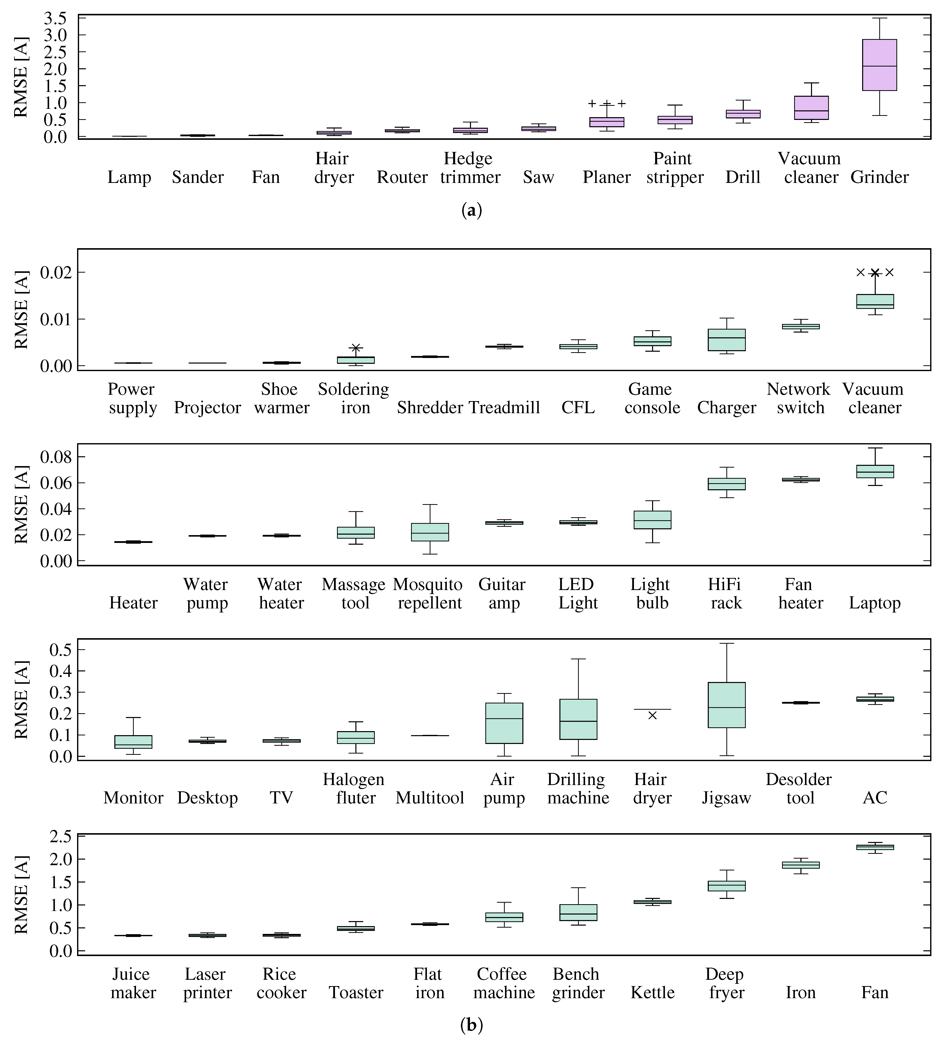
Figure 7). Similarly, the template library was fitted with the 23 most representative entries from the WHITED data set. Subsequently, all current consumption waveforms from the testing data set were processed individually, finding the parametric templates that allow for their closest reconstruction. The resulting approximation errors were logged and subsequently visualized in the box plots in
Figure 10 for absolute RMSE values and
Figure 11 where the observed RMS errors were normalized to the individual appliances’ average RMS current demands.
The diagrams confirm that our template library returns small RMSE values in comparison to the typical amplitude of the tested input cycles for many appliances. Particularly, as visible in
Figure 11, encountered errors never exceed the nominal input current of the appliance. On average, they range at
% for COOLL and
% for WHITED (i.e.,
for COOLL,
for WHITED). The large majority of the observed outliers could be traced back to the transient inrush currents observed during the first activation of the appliances (similar to the observations made in
Figure 3). It also needs to be noted, however, that the current demand of certain appliances could only be approximated with large relative errors (e.g., the monitor, air pump, or jigsaw). In these cases, the size of the template library (which only had approximately half as many entries as the number of appliances from which it was established) proved insufficient to reconstruct the appliances’ current demands accurately. Even though this reconstruction error can be slightly reduced by increasing the number of templates in the library, closely fitting templates did rarely become part of the template library due to the small number of operational cycles available for these appliances. The use of more training data is expected to improve the clustering step and lead to the extraction of even more representative templates.
5.4. Aggregated Appliance Approximation Accuracy
Our template matching approach implicitly facilitates the detection if multiple appliances are operating simultaneously, given that multiple templates are usually present in aggregated current consumption data. A second possible use case for the template library is thus to disaggregate current waveforms resulting from the concurrent operation of two of more devices. However, as the considered data sets only provide data that were measured for single appliances, it was necessary to synthetically create aggregate data through the addition of waveforms from multiple appliances. In order to avoid an unintentional bias towards certain appliance types, we have considered all possible combinations of two appliances as well as all possible combinations of three appliances, for each of the data sets. All input data sets were aligned by the zero-crossings of their voltage channels to ensure that phase shift information is correctly respected.
Figure 12 shows an excerpt of the current demand of a drill and a fan appliance over the course of a single mains period, as well as the sum of the input cycles which is subsequently used as the input data for the template matching step. The figure shows that after the identification and subtraction of the best-fitting template,
), a further contributing template could be matched to the data,
). The box plot in
Figure 12b still shows an RMSE greater than in the single-appliance case (cf.
Figure 8b). This observation can be attributed to the use of the greedy heuristic: It over-estimates the amplitude scaling factor of
, such that the difference after subtracting parameterized
from the input data is erroneously modeled by
, which does not line up with the fan’s current intake at all.
Achievable RMSE results for the complete input data (i.e., the aggregation of waveforms from two and three simultaneously operated appliances, respectively) are shown in
Figure 13. Again, we have varied the number of templates available in the library for both the COOLL and the WHITED data sets, respectively. The figure confirms our choice of the template library sizes (see
Section 5.2), as library sizes greater than our chosen values do not reduce the average RMSE much further (see also
Figure 9).
5.5. Choice of the Heuristic
In our last experiment, we investigate to what extent the choice of the greedy heuristic (cf.
Section 4.3) impacts the RMSE of the fitting step, as compared to using a solver for the optimization problem. For this test, we synthetically aggregate the current demand of all combinations of two appliances for each of the data sets. We, however, replace the greedy solver used in prior experiments by an implementation that evaluates all combinations of all templates across the full range of their parameters (discretized to amplitude steps of
and phase shift increments of
). In order to keep the computational time within reasonable bounds, we impose the constraint that at most two templates should be detected in the aggregate data; a valid assumption, given the fact that all input data is a superposition of the current waveforms of exactly two appliances. The resulting disaggregation performance for the combination of fan and drill is shown in
Figure 14. But not only in this case are the results comparable to
Figure 12, where up to three appliances were operated simultaneously; in fact, no noticeable reduction over the values shown in
Figure 13 could be observed when applying the full optimization to the whole data set. To conclude, based on the data from the COOLL and WHITED data sets, the greedy approach is sufficient to approximate the current waveforms as closely as possible, while it is inherently much less resource- and time-demanding.
