Abstract
The reflectors of a linear solar concentrator investigated in this work consisted of two plane mirrors (2MCC), and they were designed in such a way that made all radiation within the acceptance angle (θa) arrive on flat-plate absorber, after less than two reflections. To investigate the performance of an east–west aligned 2MCC-based photovoltaic (PV) system (2MCPV), a mathematical procedure was suggested based on the three-dimensional radiation transfer and was validated by the ray-tracing analysis. Analysis indicated that the performance of 2MCPV was dependent on the geometry of 2MCC, the reflectivity of mirrors (ρ), and solar resources in a site, thus, given θa, an optimal geometry of 2MCC for maximizing the annual collectible radiation (ACR) and annual electricity generation (AEG) of 2MCPV in a site could be respectively found through iterative calculations. Calculation results showed that when the ρ was high, the optimal design of 2MCC for maximizing its geometric concentration (Cg) could be utilized for maximizing the ACR and AEG of 2MCPV. As compared to similar compound parabolic concentrator (CPC)-based PV systems, the 2MCPV with the tilt-angle of the aperture yearly fixed (1T-2MCPV), annually generated more electricity when the ρ was high; and the one with the tilt-angle adjusted yearly four times at three tilts (3T-2MCPV), performed better when θa < 25° and ρ > 0.7, even in sites with poor solar resources.
1. Introduction
In recent decades, the energy consumption over the world has increased continuously due to the increase in standard of living and comfort level of peoples, which led to the increase of emission of carbon dioxide and environmental issues. The use of renewable energy resources, such as solar, wind, biomass, and geothermal can minimize the utilization of fossils fuels and environmental issues. Among all renewable sources, solar energy has gained tremendous interest due to their abundant availability in most parts of the world and because they are free from pollution [1,2]. However, compared to conventional techniques for electricity generation, the cost of the electricity from a PV system is higher and this limits its application [3]. Apart from further finding cheap materials and advance techniques for the production of solar cells, sun-tracking, and radiation concentrating techniques are widely used to reduce the cost of electricity generated by PV systems. Sun-tracking increases electricity generation from PV panels by maximizing radiation collection [4,5,6], but sophisticated devices in sun-tracking and control are required. In recent years, compound parabolic concentrators (CPCs) and V-trough concentrators were widely tested for increasing the electricity from solar cells. Compared to non-concentrating PV systems, a low concentrating PV system can reduce the cost of electricity by up to 40% [7]. Tests by Mallick et al. showed that the use of an asymmetric CPC (2.01×) increased the maximum power point of solar cells by 62% [8,9]. The experimental study by Brogren et al. indicated that the use of a CPC (3×) increased the maximum power output of solar cells by 90% [10]. A comparative study by Yousef et al. showed that, compared to similar solar panels, the electricity from a CPC (2.4×)-based PV system (CPV) was 52% and 33% higher, with and without cooling of solar cells, respectively [11]. These research studies showed that the use of CPCs can increase electricity generation of solar cells but the increments were much less than the geometric concentration ratio (Cg) of CPCs, a result mainly caused by the optical loss of CPCs due to multi-reflections of solar rays on the way to solar cells [12,13]. To simplify the fabrication of CPCs and make solar flux on solar cells more uniform, Tang proposed a concentrator (CPC-A) as the alternative to CPC where the parabolic reflectors are replaced with multi-mirrors [14].
Compared to CPCs, V-trough concentrators are easier in fabrication, and solar flux on the base is more uniform. Measurements by Sangani and Solanki indicated that the use of a V-trough concentrator (2×) increased the electricity generation of solar cells by 44% [15,16]. Theoretical and experimental studies showed that a properly designed V-trough PV system (VPV) was particularly suitable for water pumping [17,18]. A study by Vilela et al. showed that, the single axis sun-tracking VPV (2.2×) increased the ACR by a factor of 1.74 but increased the pumped water by a factor of 2.49, as compared to similar fixed solar panels [19]. Recent work of the authors showed that, as compared to fixed PV panels, the increase of AEG from inclined north–south axis multi-position sun-tracking VPV is even larger than the Cg [20]. However, V-trough is not an ideal solar concentrator, the Cg is restricted, and the optical efficiency is low [20,21,22]. To reduce the optical loss due to reflections, the reflection number of solar rays within V-trough should be restricted, but the Cg of such V-tough is restricted [20]. To increase the Cg of V-trough concentrators, Mannan and Bannerot proposed a two-mirror composite concentrator (2MCC) [23], but its optical performance was not investigated in this work. As an alternative to CPC, composite multi-mirror concentrators (n-MCC) was designed by Mullick et al. [24] based on the edge-ray principle. It is found that the maximum Cg of n-MCC increases with an increase of mirror number (n) and approaches to that of CPC as n is close to infinite. However, with an increase of n, the optical efficiency decreases, and solar flux on the absorber becomes more uneven [14].
To investigate the optical performance of a concentrator, the ray-tracing analysis is commonly employed [25,26], but it is time-consuming, even impossible when one investigates effects of geometry of a static solar concentrator on the long-term performance [14]. Similar to CPCs and V-trough concentrator, the optical performance of a linear n-MCC is uniquely determined by the projected incident angle (PIA, termed as θp) of solar rays on the cross-section [12,27,28], thus, two-dimensional radiation transfer can reasonably predict the optical performance [12]. However, the 2-D model cannot reasonably predict photovoltaic performance as the photovoltaic efficiency of solar cells is sensitive to the incident angle (IA) of solar rays on solar cells [6,12]. In this work, a 3-D radiation transfer model was developed based on the vector algebra and imaging principle of mirrors. The objective of this work was to find the optimal design of 2MCC based PV system (2MCPV) for maximizing ACR and AEG and compare its performance with a similar CPC based PV system (CPV), which was identical in Cg and θa to 2MCC.
2. Geometric Characteristics of n-MCC
Reflectors of a solar concentrator are commonly designed based on the edge-ray principle, namely, edge rays reflecting from reflectors are required to hit at the ends of a plat absorber or to be tangent to a curved absorber [29]. As shown in Figure 1, each of the two reflectors of the linear concentrator investigated here consisted of two plane mirrors, and they were designed in such a way that it made the solar ray incident on the upper end of two mirrors at θp = θa arrive on the left end of the flat-plate absorber. Obviously, for such solar concentrator (2MCC), all radiation irradiating on the mirrors at θp ≤ θa would arrive on the absorber, after less than two reflections. According to the reflection law of light, the geometry of 2MCC should be subjected to (the width of the absorber was set to be 1 for simplifying the analysis):
where h = h1 + h2 is the height of 2MCC, h1 and h2 are the vertical height of lower and upper mirrors, respectively, and they are given by:
Cg = 2(h1 + h2)tanα2 − 1 = 2htanα2 − 1
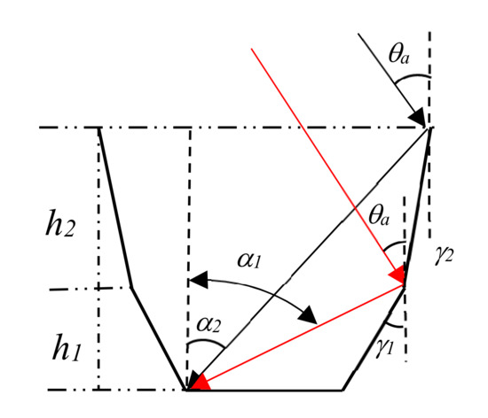
Figure 1.
Scheme of 2MCC.
Cg = 2hntanαn − 1
The vertical height (h1) of the bottom mirror is given by Equation (2), and that of the jth mirror counting from the bottom is given by:
αj = θa + 2γj (j = 1, 2, …, n)
It is known from Equations (1)–(3) that, given θa, the geometry of 2MCC is dependent on γ1 and γ2, thus, a set of γ1 and γ2 for maximizing Cg could be found through the iterative calculations. Similarly, Cg of n-MCC was sensitive to the tilt-angle of n-mirrors and a set of γi (i = 1, 2, …, n) for maximizing Cg could be found though multi-loops iterative calculations.
As seen in Figure 2, given θa, the Cg of n-MCC increased with an increase of mirror numbers (n), as indicated by Mullick [24]. The optimal geometry of 2MCC and 3MCC for maximizing Cg is presented in Figure 3. It can be seen that the optimal tilt-angle of bottom mirror of n-MCC for maximizing Cg (termed as γ1,g) was highly sensitive to θa and decreased with an increase of θa, but that of the top mirror (termed as γn,g) was weakly sensitive to θa, furthermore, γ1,g was always larger than nγn,g. It was also seen that the maximum Cg of 2MCC and 3MCC decreased with an increase of θa. To ensure Cg > 2, the θa of 2MCC and 3MCC should be less than 17.7° and 21.3°, respectively. Just like CPCs, linear n-MCC was commonly oriented in the east–west direction. Therefore, to ensure Cg > 2 and the sun within θa of 2MCC and 3MCC for more than 7 h in all days of a year, the tilt-angle of 2MCCs’ aperture should be yearly adjusted four times at three tilts, and that of 3MCC’s aperture should be adjusted more than two times in a year [27,30].
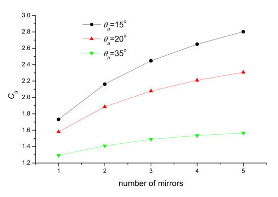
Figure 2.
Maximum geometric concentration of n-MCC.
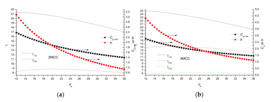
Figure 3.
(a) Optimal geometry of 2MCC and (b) 3MCC for maximizing Cg.
3. Mathematical Procedure to Predict the Performance of 2MCPV
The 2MCC orientation was assumed to be in the east–west direction and its aperture to be tilted at β from the horizon. To make the analysis easier, a coordinate system with the x-axis normal to the aperture, the y-axis parallel to the horizon and pointing to the east, and the z-axis pointing to the northern sky was employed (see Figure 4). In this coordinate system, the unit vector of the incident solar rays was expressed by [6,31]:
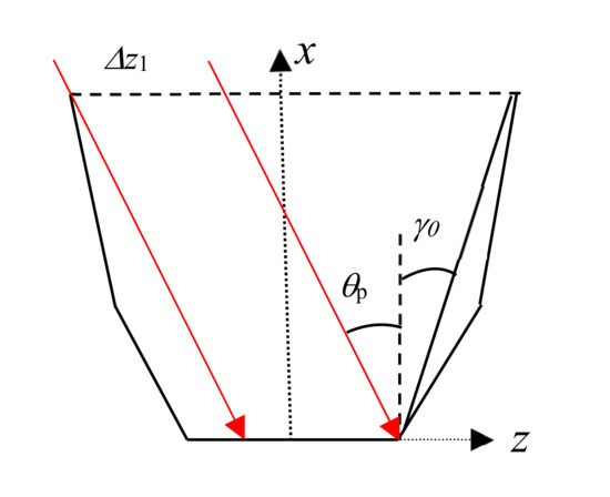
Figure 4.
Radiation directly irradiating on the absorber.
For the 2MCC symmetric about the normal to aperture, the performance for solar rays ns = (nx, ny, ± nz) was identical. Therefore, to simplify the analysis, it was assumed that solar rays were always incidental onto the right mirrors (see Figure 4), namely, nswas always set to be
3.1. Optical and Photovoltaic Efficiency of 2MCC-Based PV System
The radiation on the absorber of 2MCC include five components—radiation directly incident on the absorber (I1) and those irradiating first on four mirrors and then arriving on the absorber after reflections (I2, I3, I4, I5). Therefore, the optical efficiency of 2MCC was expressed by:
where Iap is the radiation incident on the aperture; fi (i = 1, 2, 3, 4, 5) is the energy fraction of the radiation on the absorber contributed by Ii. Similarly, the PV conversion efficiency of the 2MCC-based PV system (2MCPV) was expressed by:
where Pi (i = 1, 2, 3, 4, 5) is the electricity generated by Ii, and the ηi (i = 1, 2, 3, 4, 5) is the PV conversion efficiency of 2MCPV contributed by Pi.
f = (I1 + I2 + I3 + I4 + I5)/Iap = f1 + f2 + f3 + f4 + f5
η = (P1 + P2 + P3 + P4 + P5)/Iap = η1 + η2 + η3 + η4 + η5
3.1.1. Radiation Directly Irradiating on the Absorber
As seen from Figure 4, the absorber was fully irradiated when θp ≤ γ0 and partially irradiated as γ0 < θp < α2, thus, f1 = I1/Iap = Δz1/Cg was calculated by:
The electricity from 2MCPV generated by I1 was given by P1 = I1ηpv(θin,1), thus, the one had:
where ηpv(θin,1) is the PV efficiency of solar cells as a function of θin,1. The IA of the solar rays directly irradiating on the solar cells is given by:
as the unit vector of the normal to solar cells of 2MCPV is nabs = (1,0,0) in the suggested coordinate system. The electricity from 2MCPV is generally affected by many factors such as cell temperature and electricity load [32]. To simplify the analysis and facilitate investigating the effects of the geometry of 2MCC on the PV performance of 2MCPV, it was assumed that, except the IA (θin), effects of the other factors on the PV efficiency of solar cells were not considered, and the PV efficiency of solar cells in percentage was subjected to the correlation, as follows [33]:
η1 = f1ηpv(θin,1)
3.1.2. Radiation Irradiating on Right Lower Mirror and Arriving on the Absorber
According to the geometric characteristics of 2MCC and the imaging principle of mirrors, one knows that all radiation irradiating on the right lower mirror arrives on the absorber after one reflection when θp ≤ θa, whereas for the case of θp > θa, a fraction of radiation would arrive after more than one reflection, as seen in Figure 5 [22]. For the case of θp ≤ θa, the radiation incident on right lower mirror and arriving on the absorber after reflection was I2 = Δz2ρ, hence, one had:
where ηpv(θin,21) is the PV efficiency of solar cells as the function of θin,21 and is determined by Equation (16). The IA of the solar ray on solar cells in this case (see left of Figure 5) was given by:
as the unit vector of the normal to first right-image of the absorber formed by lower mirrors is (cos2γ1,0,sin2γ1), due to the first right-image making an angle of 2γ1 from the absorber [12,20,22].
f2 = Δz2ρ/Cg = h1(tanθp + tanγ1)ρ/Cg (θp ≤ θa)
η2 = Δz2ρηpv(θin,21)/Cg = f2ηpv(θin,21) (θp ≤ θa)
cosθin,21 = ns · (cos2γ1,0,sin2γ1)= nx cos2γ1+nz sin2γ1
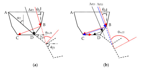
Figure 5.
Radiation irradiating on right lower mirror (BD) and arriving on absorber after reflections: (a) θp ≤ θa; (b) θp > θa.
When solar rays are incident on the aperture at θp > θa, a fraction of radiation incident on the right lower mirror might arrive on the absorber after more than one reflection, as shown in the right side of Figure 5. The PIA of solar rays on the absorber after multi-reflections within the V-trough formed by the two lower mirrors was equal to (2γ1k + θp) and was required to be less than 90°, thus the maximum reflection number of solar rays within the V-trough was given by:
as multi-reflections take place only when θp > θa. Calculations showed that γ1 of the 2MCC optimized for maximizing the Cg was larger than 17° for θa < 40°, thus kmax was 2. This meant that more than two reflections would not take place for θa < 40°. In practical applications, θa should be less than 40° to ensure Cg > 1.3. Therefore, f2 and η2 for the case of θp > θa could be calculated by:
where Δz21 and Δz22 are the radiation that irradiates on the right lower mirror and arrives on the absorber after one and two reflections, respectively (see Figure 5). They were calculated by [20,22]:
where FR1 and FR2 are the z-coordinate differences between two ends of the right first and second images irradiated by the incident radiation, respectively, and they were given by:
where
kmax = Int [(90 − θp)/2γ1] ≤ Int [(90 − θa)/2γ1]
f2 = (Δz21 ρ + Δz22 ρ 2)/Cg
η2 = [Δz21 ρ ηpv(θin,21) + Δz22 ρ2ηpv(θin,22)]/Cg
Δz21 = FR,1[1 − tan(2γ1)tanθp]
Δz22 = FR,2[1 − tan(4γ1)tanθp]
The C1 = 2h1tanα1 − 1 was the geometric concentration of 1MCC (V-trough formed by two lower mirrors of 2MCC). The θin,22 in Equation (22) was the IA of the solar rays after two reflections and was determined by:
as the unit vector of the normal to second right-image was expressed by (cos4γ1, 0, sin4γ1). It was noted that f2 and η2 were set to be zero when θp ≥ 90 − 4γ1 or θp ≥ θmax. The θmax was the angle of the edge-ray that irradiated on lower mirrors and arrived on the absorber, after more than one reflection, and was determined by:
where θ1 and θ2 are, respectively, the angle of rays passing the left/right-end of the aperture and the right/left-end of first and second right/left images, and was calculated by:
cosθin,22 = ns· (cos4γ1,0,sin4γ1) = nx cos4γ1 + nz sin4γ1
θmax = Max(θ1,θ2)
tanθ1 = (0.5 + 0.5Cg + cos2γ1)/(h + sin2γ1)
tanθ2 = (0.5 + 0.5Cg + cos2γ1 + cos4γ1)/(h + sin2γ1 + sin4γ1)
3.1.3. Radiation Irradiating on the Left Lower Mirror and Arriving on the Absorber
First, it should be addressed that all radiation irradiating on the left mirrors would arrive on the absorber after less than two reflections, because θp was negative, thus, it was less than θa, as the radiation was always assumed to be incident onto the right mirrors, in this work. As seen in Figure 6, the left lower mirror was fully irradiated when θp ≤ γ2, and partially irradiated for γ2 < θp < γ0. Thus one had:
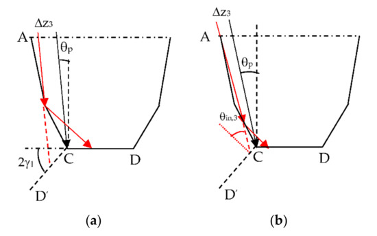
Figure 6.
Radiation irradiating on left lower mirror and arriving on the absorber after reflection: (a) θp ≤ γ2; (b) γ2 < θp < γ0.
The IA of the solar rays after reflection was given by:
as the unit vector of the normal to the image formed by left lower mirror was (cos2γ1,0, −sin2γ1) [12]. Therefore, the η3 was given by:
cosθin,3 = ns· (cos2γ1,0, −sin2γ1) = nx cos2γ1 − nz sin2γ1
η3 = f3ηpv(θin,3)
3.1.4. Radiation Irradiating on Left Upper Mirror and Arriving on Solar Cells
As shown in Figure 7, the CD’ was the image of the lower mirror (CD) formed by the upper mirror (AC). According to the imaging principle of mirrors, one knows that when θp ≥ , all radiation incident on the upper mirror would redirect onto the lower mirror first and then redirect onto solar cells; whereas for θp < , radiation incident on the upper part (AE) of the upper mirror directly redirected onto solar cells and that on the lower part (EC) redirected onto the lower mirror (CD) first, then redirected onto the solar cells. Therefore, f4 could be calculated by:
where is the angle of line relative to the x-axis and determined by:
as the image of lower mirror made an angle of γ1 − 2γ2 relative to x-axis. The in Equation (36) was the width of image and was given by = h1/cosγ1. The hEC in Equation (34) was the vertical height of the mirror EC and was calculated by:
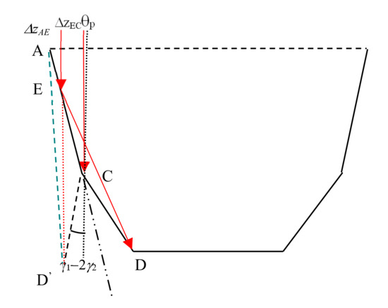
Figure 7.
The radiation irradiating on the left upper mirror and arriving on the absorber.
The IA of the solar rays directly redirecting onto the solar cells was calculated by:
as the vector of the normal to the image of solar cells formed by left upper mirror was (cos2γ2,0, −sin2γ2). The IA of the solar rays redirecting onto the lower mirror (CD) first, then onto the solar cells was calculated by [12]:
cosθin,41 = ns· (cos2γ2,0, −sin2γ2) = nx cos2γ2 – nz sin2γ2
cosθin,42 = nx cos (2γ1 − 2γ2) + nz sin (2γ1 − 2γ2)
On knowing θin,41 and θin,42, one could calculate η4 as follows:
3.1.5. Radiation Irradiating on the Right Upper Mirror and Arriving on the Absorber
As seen in Figure 8, the methods through which the solar rays irradiate on the right upper mirror and arrive on the absorber, differed for different θp and were divided into four cases, as follows.
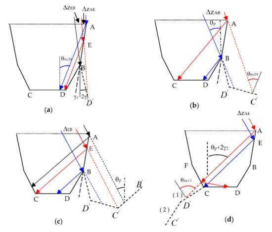
Figure 8.
The radiation irradiating on the right upper mirror and arriving on the absorber. (a) θp < γ1 − 2γ2; (b) γ1 − 2γ2 ≤ θp ≤ θa; (c) θa < θp ≤ θa + 2(γ1 − γ2); and (d) radiation on the absorber reflecting from the right upper-mirror first and then from left lower-mirror for θa < θp < θmax − 2γ2.
- Case A: θp < γ1 − 2γ2
As shown in Figure 8a, the image of the right lower mirror (BD) formed by the right upper mirror made an angle of γ1 − 2γ2 from the x-axis, therefore, when the solar rays were incident on the upper mirror at θp < γ1 − 2γ2, the radiation irradiating on the upper part (AE) of the mirror directly redirected onto the solar cells, and that on the lower part (EB) redirected onto the lower mirror (BD) first, and then onto the solar cells. The f5 and η5 in this case were calculated by
The vertical height of EB was given by:
The IA of the solar rays on the solar cells reflecting from AE (θin,51) and those reflecting from EB (θin,52) were calculated by [12]:
cos θin,51 = ns ·(cos2γ2,0, sin2γ2) = nx cos2γ2 + nz sin2γ2
cosθin,52 = nx cos(2γ1 − 2γ2) – nz sin(2γ1 − 2γ2)
- Case B: γ1 − 2γ2≤θp ≤ θa
In this case, all radiation incident on the right upper mirror directly redirected onto the solar cells, as shown in Figure 8b, therefore, one had:
f5 = ΔzABρ/Cg = h2(tanγ2 + tanθp)ρ/Cg
η5 = f5ηpv(θin,51)
- Case C: θa < θp < θmax − 2γ2
As shown in Figure 8c,d, the angle of line AC relative to the x-axis was equal to α2 and the angle of rays reflecting from right upper mirrors was θp + 2γ2. Therefore, when α2 < θp + 2γ2 < θmax, i.e., θa < θp < θmax − 2γ2, the radiation incident on the lower part (EB) of the right upper mirror would arrive on the solar cells after one reflection and that on the upper part (AE) would redirect onto the left lower mirror first then onto the absorber, after more than one reflection. Thus, the radiation incident on right upper mirror at θa < θp < θmax − 2γ2 and arriving on the solar cells included two components—directly redirecting on solar cells (I5,1) and redirecting to the left lower mirror first, then onto the solar cells (I5,2). The I5,1 could be calculated by:
as the IA of the ray reflecting from the lower end (B) of the right upper mirror should be less than α1, namely θp + 2γ2 ≤ θa + 2γ1 (θp ≤ θa + 2γ1 − 2γ2), thus, no radiation arrived on the solar cells after reflection from the right upper mirror, when θp > θa + 2γ1 − 2γ2. The electricity generated by I5,1 was given by:
P5,1/Iap = I5,1 ηpv(θin,51)
As shown in Figure 8d, when θa < θp < θmax − 2γ2, the rays reflecting from the upper part (AE) of the right upper mirror redirected onto the left lower mirror first and then onto the solar cells, after more than one reflection. The I5,2 and P5,2 were calculated by:
where ΔzL1 and ΔzL2 were the radiation reflecting from the right upper mirror and arriving on the solar cells after one- and two-reflection, respectively, and were calculated as follows:
where FL,1 and FL,2 are the z-coordinate differences between the two ends of the first and second left-image of the absorber irradiated by the radiation from AB, respectively, and they were given by:
where
I5,2/Iap = (ΔzL1ρ2 + ΔzL2ρ3)/Cg
P5,1/Iap = [ΔzL1ρ2ηpv(θin,L1) + ΔzL2ρ3 ηpv(θin,L2)]/Cg
ΔzL1 = FL1cos(θp + 2γ2) [1 − tan(2γ1)tan(θp + 2γ2)]/cosθp
ΔzL2 = FL2cos(θp + 2γ2) [1 − tan(4γ1)tan(θp + 2γ2)]/cosθp
The IA of the solar rays from AE and arriving on the solar cells after one- and two-reflection was equal to that of rays from AE on the first and second left-image of solar cells, formed by the lower mirrors, respectively, and they were calculated by [12]:
as the unit vector of the ray reflecting from AE was given by rAE = (cos2γ2, ny, nz + 2cosθin,AEcosγ2) and the IA of the solar rays on the AE was given by cosθin,AE = ns ·(sinγ2,0, −cosγ2) = nx sinγ2 − nz cosγ2. It was noted that ΔzL1 = 0 when θp > 90° − 2γ1 − 2γ2 and ΔzL2 = 0 as θp > 90° − 4γ1 − 2γ2, because the PIA of the solar rays from the AE on the first and second left-images was equal to θp + 2γ2 + 2γ1 and θp + 2γ2 + 4γ1, respectively, and they were required to be less than 90°. On obtaining I5,1, P5,1, I5,2 and P5,2, one had:
cosθin,L1 = rAE ·(cos2γ1,0, −sin2γ1) = nx cos(2γ1 + 2γ2) + nz sin(2γ1 + 2γ2)
cosθin,L2 = rAE ·(cos4γ1,0, −sin4γ1) = nx cos(4γ1 + 2γ2) + nz sin(4γ1 + 2γ2)
f5 = (I5,1 + I5,2)/Iap
η5 = (P5,1 + P5,2)/Iap
The analysis in above showed that the optical efficiency of 2MCPV only depended on θp, but the PV efficiency depended on θp and nx.
3.2. Annual Optical and Photovoltaic Performance of 2MCPVs
It was assumed that the diffuse radiation from the sky was isotopic and that reflection from the ground was not considered. Therefore, the radiation on the unit area of the solar cells of 2MCPV at any moment of a day could be calculated by:
as the IA of the solar rays on the aperture was given by cosθap = ns ·(1,0,0) = nx. The electricity generated by the unit area of the solar cells of 2MCPVs at any time of a day was calculated by:
where Ib is the intensity of beam radiation, the , a control function, is 1 for cosθap > 0 otherwise zero. The Iabs,d in Equation (61) is the sky diffuse radiation collected by the unit area of the solar cells and could be calculated on the basis of the two-dimensional sky diffuse radiation, as follows:
as the optical efficiency of the linear 2MCPV was only dependent on θp, and the directional intensity of the sky diffuse radiation on the cross-section of the east–west oriented 2MCPV was isotropic [6] for the isotropic sky diffuse radiation and was equal to 0.5Id [13]. Pd in Equation (62) was the electricity generated by Iabs,d and should be calculated on the basis of the three-dimensional sky diffuse radiation, as follows [12]:
as the PV efficiency of 2MCPV depended on θp and nx, and the electricity generated by diffuse radiation from a finite element of the sky dome was dPd = idCgcosθηsinθ with id = πId/3 [12]. The φ0 in Equation (64) was related to θ by:
The Id in Equations (63)–(64) was the sky diffuse radiation on the horizon. For a given 2MCPV, Cd in Equation (63) and Cd,pv in Equation (64) depended on β and could be numerically calculated. The radiation on the unit area of the solar cells of 2MCPV in a day could be estimated by integrating Iabs over the daytime of the day, as:
The daily electricity from unit area of the solar cells was estimated by:
where the Hd in Equations (66)–(67) is the daily sky diffuse radiation on the horizon, t0 is the sunset time on the horizon in a day.
At any time of a day, the position of the sun in terms of ns could be determined, then f and η could be calculated. Therefore, given the time variation of Ib and Hd in a day, Hday, and Pday could be numerically calculated, then summing Hday and Pday and all days of a year yields the ACR on the solar cells (Sa) and AEG (Pa) of 2MCPV.
4. Methodology
To evaluate the mathematical model suggested in this work, the optical efficiency of the 2MCC calculated, based on the mathematical method in this work were compared with those from the ray-tracing analysis, with the aid of the commercial Tracepro software provided by Lambda Research, NASA of US [14].
To find the optimal geometry of 2MCPV for maximizing Sa and Pa, the monthly global radiation on the horizon in Beijing (λ = 39.95°, a site with abundant solar resources) and Chongqing (λ = 29.5°, a site with poor solar resources) were used for calculations [34]. Given the global radiation on the horizon for a month, the monthly average daily radiation on the horizon was estimated by dividing the monthly value over the days of the month, then, the monthly average Hd and the time variation of Ib in a day of the month were estimated, based on correlations proposed by Collares–Pereira and Rabl [35]. The time interval for calculating the daily radiation on the solar cells and the daily electricity from 2MCPV was set to be 1 min. The step of θ and φ for calculating Cd,pv in Equation (64) was set to be 0.1°, and the step of γ1 and γ2 for finding the optimal geometry of 2MCC for maximizing Sa and Pa was taken to be 0.1°. To fully investigate the performance of 2MCPV, 2MCPVs with the aperture’ tilt-angle being yearly fixed (1T-2MCPV) and yearly adjusted, four times, at three-tilts (3T-2MCPV) were considered. For 1T-2MCPV, the tilt-angle (β) was set to be site latitude (λ). For 3T-2MCPV, β = λ during the period of 22 days, before and after equinoxes, and was adjusted to be λ − α and λ + α in summers and winters, respectively [22,30]. To ensure solar rays within θa at the solar-noon in the days (δ = ±8.5°) when the tilt-angle was adjusted, the value of α for 3T-2MCPV was set to be 22° for θa ≥13.54° and α = θa + 8.5 for θa < 13.54° [30].
To compare the performance of 2MCPV with CPC-based PV systems (CPV), the AEG, generated by similar CPV, which was identical in the Cg and θa to 2MCC optimized for maximizing Cg, was calculated based on the mathematical model proposed by Tang et al. [12].
5. Results and Discussion
5.1. Comparisons of Optical Efficiency between 2MCC and Similar CPC
It can be seen from Figure 9 that the optical efficiency of 2MCC and similar CPC expected by mathematical models developed in the present and previous works [12], were almost identical to those from the ray-tracing analysis, indicating that they could reasonably be used to predict the optical performance of 2MCC and CPC, respectively. As compared to similar truncated CPC, the optical efficiency of 2MCC was slightly lower as θp ≤ θa because α2 of 2MCC was much less than the edge-ray angle (θt) of the truncated CPC (see Figure 10). Thus, more radiation directly irradiated on the solar cells, but it was higher when θp was slightly larger than θa, because a fraction of radiation irradiating on the right mirrors of the 2MCC arrived on the absorber after reflections but the radiation on the right parabola of CPC eventually escaped away from the aperture. It was also seen that when θp > θmax, f = 0 for 2MCC but not for the truncated CPC, as θt of the similar truncated CPC was much larger than the θmax of 2MCC (see Figure 10), indicating that CPC was more favorable for the collection of sky diffuse radiation, as compared to 2MCC.
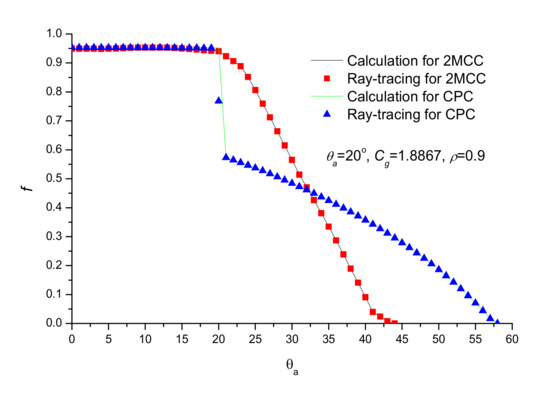
Figure 9.
Comparisons of optical efficiency between theoretical calculation and ray-tracing analysis.
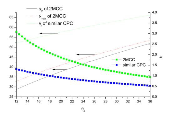
Figure 10.
Comparisons of the edge-ray angle and height between 2MCC optimized for maximizing Cg and similar truncated CPC.
5.2. Optimal Design of 2MCC
As aforementioned, given θa, the geometry of 2MCC was uniquely determined by γ1 and γ2. Thus, the performance of 2MCPV also depended on γ1 and γ2, and a set of γ1 and γ2 for maximizing ACR (Sa) and ARG (Pa) could be respectively found through iterative calculations. Figure 11 presents the optimal geometry of 1T-2MCPV optimized for maximizing Sa and Pa in Beijing (upper two sub-plots) and Chongqing (down two sub-plots). It was observed that the γi,Sa (i = 1, 2), the optimal γi for maximizing Sa, and γi,Pa (i = 1, 2), the optimal γi for maximizing Pa, increased with a decrease of ρ, and for a given ρ, γi,Sa > γi,Pa and γi,Sa > γi,g. Increasing γi, especially γ1, resulted in more radiation directly irradiating on the solar cells, and decreasing γi reduced the IA of the solar rays on the solar cells, thus improving the PV efficiency of the solar cells. It was also seen that γ1,Pa < γ1,g and γ2,Pa ≈ γ2,g for high ρ (ρ = 0.9), whereas for low ρ (ρ = 0.7), γ1,Pa ≈ γ1,g and γ2,Pa > γ2,g. It was also shown that γ1,Sa and γ1,Pa were highly sensitive to θa but γ2,Sa and γ2,Pa were weakly sensitive to θa. Geometric concentrations of 1T-2MCC optimized for maximizing Cg (termed as Cg,max), Sa (termed as Cg,Sa), and Pa (termed as Cg,Pa) are presented in Figure 12. It shows that Cg,Sa and Cg,Pa were almost identical, and they were close to Cg,max for ρ = 0.9 but were about 1–1.5% and 1.2–1.8% lower for ρ = 0.7 in Beijing and Chongqing, respectively.
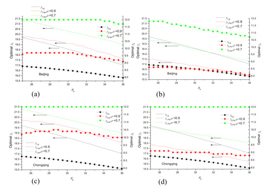
Figure 11.
Optimal geometry of 1T-2MCPV: (a) to maximize Sa in Beijing; (b) to maximize Pa in Beijing; (c) to maximize Sa in Chongqing; (d) to maximize Pa in Chongqing.
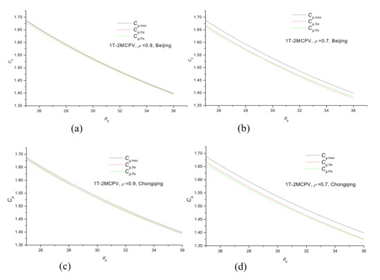
Figure 12.
Geometric concentration of 1T-2MCPV optimized for maximizing Sa and Pa: (a) for ρ = 0.9 in Beijing; (b): for ρ = 0.7 in Beijing; (c): for ρ = 0.9 in Chongqing; (d): for ρ = 0.7 in Chongqing.
Optimal design of 2MCPV with the tilt-angle of the aperture being yearly adjusted four times at three tilts (3T-2MCPV) is presented in Figure 13. Similar to 1T-2MCPV, for a given θa, the γi,Sa and γi,Pa increased with a decrease of ρ, and given ρ, γi,Sa > γi,Pa. It showed that for 3T-2MCPV, optimized for maximizing Sa, the γ1,Sa was close to γ1,g, while γ2,Sa ≈ γ2,g for high ρ but γ2,Sa > γ2,g for low ρ; whereas for 3T-2MCPV optimized for maximizing Pa, γ1,Pa < γ1,g, except in Chongqing for the case of θa > 24° and ρ = 0.7, while γ2,Pa ≈ γ2,g for high ρ and γ2,Pa > γ2,g for low ρ. It was also found that Cg,Sa and Cg,Pa were almost identical, and they were close to Cg,max for ρ = 0.9 but slightly lower for ρ = 0.7, as shown in Figure 14.
Figure 13.
Optimal design of 3T-2MCPV: (a) to maximize Sa in Beijing; (b) to maximize Pa in Beijing; (c) to maximize Sa in Chongqing; (d) to maximize Pa in Chongqing.
Figure 14.
Geometric concentration of 3T-2MCPV optimized for maximizing Sa and Pa: (a) for ρ = 0.9 in Beijing; (b) for ρ = 0.7 in Beijing; (c) for ρ = 0.9 in Chongqing; (d) for ρ = 0.7 in Chongqing.
5.3. Performance of 2MCPV
Figure 15 presents the ACR of 1T-2MCC optimized for maximizing Sa, Cg, and that of similar 1T-CPC. It can be seen that the Sa collected by 1T-2MCC optimized for maximizing Sa (termed as Sa,max) and that collected by 1T-2MCC optimized for maximizing Cg (termed as Sa,g) almost linearly decreased, with an increase of θa. For ρ = 0.9, Sa,g was almost identical to Sa,max, and for ρ = 0.7, Sa,g were respectively about 99% and 98% of Sa,max (see lines Sa,g/Sa,max), in Beijing and Chongqing. This meant that 1T-2MCC optimized for maximizing Cg, could be regarded as the optimal geometry for maximizing Sa, when ρ was high. It also showed that, in the site with abundant solar resources such as Beijing, the Sa,cpc, collected by similar 1T-CPC, was slightly lower than Sa,g and Sg,max for ρ = 0.9 but was higher for ρ = 0.7; whereas in the sites with poor solar resources such as in Chongqing, the Sa,cpc was slightly higher than Sa,max, except when θa < 28° and ρ = 0.9. This indicated that as compared to similar 1T-CPC, the 1T-2MCC even annually collected more radiation in the sites with abundant solar sources, because a fraction of radiation incident on the mirrors of 2MCC at θp > θa arrived on the absorber, but all radiation incident on the parabola of CPCs at θp > θa escaped away from the aperture of CPCs.
Figure 15.
ACR of 1T-2MCC optimized for maximizing Sa, Cg, and that by similar 1T-CPC: (a) in Beijing for ρ = 0.9; (b) in Beijing for ρ = 0.7; (c) in Chongqing for ρ = 0.9; (d) in Chongqing for ρ = 0.7.
The AEG from 1T-2MCPV optimized for maximizing Pa and Cg as well similar 1T-CPC based PV system (1T-CPV) is presented in Figure 16. Similar to ACR of 1T-2MCC, the Pa,max (AEG from 1T-2MCPV optimized for maximizing Pa) and Pa,g (AEG from 1T-2MCPV optimized for maximizing Cg) linearly deceased with an increase of θa. For ρ = 0.9, Pa,g was almost identical to Pa,max, while for ρ = 0.7, Pa,g were, respectively, about 99% and 98.3% of Pa,max (see lines Pa,g/Pa,max) in Beijing and Chongqing. It showed that for ρ = 0.9, the Pa,g was slightly larger than Pa,cpv (AEG from similar 1T-CPV), whereas, for ρ = 0.7, Pa,g was close to Pa,cpv in Beijing but was slightly less in Chongqing. These results indicated that 1T-2MCPV optimized for maximizing Cg could also be regarded as the one for maximizing Pa for high ρ, and 1T-2MCPV with a high ρ generated more electricity annually, as compared to similar 1T-CPV.
Figure 16.
AEG from 1T-2MCPV optimized for maximizing Pa, Cg, and that from similar 1T-CPV: (a) in Beijing for ρ = 0.9; (b) in Beijing for ρ = 0.7; (c) in Chongqing for ρ = 0.9; (d) in Chongqing for ρ = 0.7.
The optical performance of 3T-2MCC is shown in Figure 17. It was seen that for ρ = 0.9, the Sa,g was almost identical to Sa,max, while for ρ = 0.7, Sa,g were respectively about 99.6% and 99% of Sa,max in Beijing and Chongqing. This meant that the 2MCC optimized for maximizing Cg could be regarded as the optimal ρ design of 3T-2MCC for maximizing Sa when ρ > 0.7. For ρ = 0.9, Sa,g and Sa,cpc were almost identical, whereas for ρ = 0.7, Sa,g was slightly less than Sa,cpc. Figure 18 shows the PV performance of 3T-2MCC and similar 3T-CPC-based PV systems. It can be seen that Pa,g was very close to Pa,cpv, even for ρ = 0.7. For ρ = 0.9, Pa,g > Pa,cpv especially for small θa, whereas for ρ = 0.7, Pa,g > Pa,cpv in Beijing as θa < 35° and in Chongqing when θa < 25°. These results indicate that the 2MCC optimized for maximizing Cg could also be regarded as the optimal design of 3T-2MCPV for maximizing Pa for ρ > 0.7, and compared to 3T-CPV, 3T-2MCPV was more favorable in the AEG for θa < 25° and ρ > 0.7.
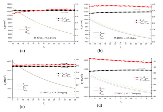
Figure 17.
ACR of 3T-2MCC optimized for maximizing Sa, Cg, and that by similar 3T-CPC: (a) in Beijing for ρ = 0.9; (b) in Beijing for ρ = 0.7; (c) in Chongqing for ρ = 0.9; (d) in Chongqing for ρ = 0.7.
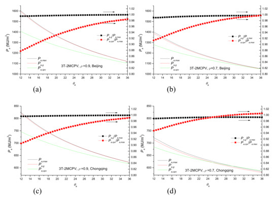
Figure 18.
AEG from 3T-2MCPV optimized for maximizing Pa, Cg and that from similar 3T-CPV: (a) in Beijing for ρ = 0.9; (b) in Beijing for ρ = 0.7; (c) in Chongqing for ρ = 0.9; (d) in Chongqing for ρ = 0.7.
In practical applications, θa should be larger than 35.5° for 1T-2MCC and 1T-CPC and 13.5° for 3T-2MCC and 3T-CPC, to ensure that they efficiently operate for at least 7 h, in all days of a year. Therefore, as compared to similar CPV, the 1T-2MCPV was more favorable in the AEG and ACR, when ρ was high, such as ρ = 0.9, but the situation was reversed when ρ was low, such as ρ = 0.7, while 3T-2MCPV annually collected almost identical radiation but generated more electricity as θa < 25° and ρ > 0.7.
6. Conclusions
In this work, the design of multi-mirror composite concentrator with flat-plate absorber was addressed. The analysis indicated that, given the acceptance angle (θa), the geometry of n-MCC was uniquely determined by the tilt-angle (γi, i = 1, 2, …, n) of all mirrors, and a set of γi (i = 1, 2, …, n) for maximizing the geometric concentration (Cg) could be found through multi-loop iterative calculations. Results showed that, given θa, the Cg increased with an increase of the mirror number (n), and the optimal tilt angle (γ1,g) of the bottom mirror for maximizing Cg was larger than n times that of the top mirror (i.e., γ1,g > nγn,g). Results also indicated that, given n, the maximum geometric concentration (Cg,max) of n-MCC decreased with an increase of θa, and the θa of 2MCC and 3MCC must be, respectively, less than 17.7° and 21.3°, to ensure Cg > 2.
To investigate the performance of a 2MCC-based PV system (2MCPV) and an optimal design for maximizing ACR and AEG, a three-dimensional radiation transfer model was developed by means of imaging principle of mirrors and vector algebra. Results showed that the optical efficiencies of 2MCC obtained by theoretical calculations and those from the ray-tracing analysis were in complete agreement, thus, it allowed to accurately predict the optical performance of 2MCC.
Analysis indicated that the optimal and photovoltaic performance of 2MCPV was dependent on the geometry of 2MCC, and the reflectivity of the mirrors (ρ) and solar resources in a site. Thus, given ρ, an optimal geometry of 2MCC for maximizing Sa and Pa in a site can be respectively found through iterative calculations. Calculations showed that when ρ was high, such as ρ = 0.9, the Cg of 1T- and 3T-2MCPV for maximizing Sa and Pa were almost identical to that of 2MCC for maximizing Cg. Hence, 2MCC optimized for maximizing Cg could be regarded as the one for maximizing Sa and Pa of 1T- and 3T-2MCPV. For 1T-2MCPV, the ACR and AEG linearly decreased with an increase of θa, as compared to similar 1T-CPV, it yearly collected more radiation and generated more electricity when the ρ was high. Whereas for 3T-2MCPV, as compared to similar 3T-CPV, it annually collected more radiation when the ρ was high and generated more electricity when θa < 25° and ρ > 0.7, even in the sites with poor solar resources.
The transfer of radiation within 3MCC was extremely complex, and the theoretical investigation in this work was only focused on 2MCC. It was believed that, the results obtained in this work were also helpful for design and application of 3MCC and even n-MCC.
Author Contributions
R.T., the sponsor of the work; G.L. is responsible for the development of 3-D mathematical model and calculations; Y.Y., responsible for the ray-tracing analysis. All authors have read and agreed to the published version of the manuscript.
Funding
This research was funded by Nature Science Foundation of China, 51466016.
Conflicts of Interest
The authors declare no conflict of interest.
Glossary
| Cg | geometric concentration ratio (dimensionless) |
| Cd | concentration coefficient of 2MCC for sky diffuse radiation (dimensionless) |
| Cd,pv | PV conversion coefficient of 2MCPV for sky diffuse radiation (dimensionless) |
| FR,k | z-coordinate differences between two ends of kth right image of the absorber irradiated by the incident radiation (m) |
| FL,k | z-coordinate differences between two ends of kth left image of the absorber irradiated by the radiation reflecting from right upper mirror (m) |
| f | optical efficiency (dimensionless) |
| H | daily radiation (J/m2) |
| h | height of 2MCC and 3MCC (m) |
| hi | height of ith mirror counted from the bottom (m) |
| I | instantaneous radiation intensity (W/m2) |
| n | unit vector; number of mirrors |
| ns | unit vector of incident solar rays |
| kmax | maximum reflection number of solar rays incident on the lower mirror and arriving on the absorber |
| Pa | Annual electricity generation (MJ/m2) |
| Sa | Annual collectible radiation (MJ/m2) |
| t | solar time (s) |
| Greek Letters | |
| αi | incident angle on the absorber of rays reflecting from ith mirror when θp = θa (rad.) |
| β | tilt-angle of CPVs’ aperture from the horizon (rad.) |
| Δz | coordinate difference of z-component (m) |
| δ | declination of the sun (rad.) |
| η | PV conversion efficiency of 2MCPVs (dimensionless) |
| ηpv | PV conversion efficiency of solar cells as a function of IA (dimensionless) |
| γ | tilt-angle of mirrors or any line relative to x-axis (rad.) |
| λ | site latitude (rad.) |
| θa | acceptance half-angle of 2MCC and CPC (rad.) |
| θap | incident angle of solar rays on the aperture of 2MCPV (rad.) |
| θmax | angle of edge-ray irradiating on lower mirrors and arriving on the absorber after reflections (rad.) |
| θin | incident angle of solar rays on solar cells (rad.) |
| θp | projected angle of incident solar rays on the cross-section of a linear 2MCC (rad.) |
| θt | edge-ray angle of truncated CPC (rad.) |
| ρ | reflectivity of mirrors (dimensionless) |
| ω | hour angle (rad.) |
| Subscripts | |
| 0 | sunset |
| a | annual |
| abs | absorber or solar cells of 2MCPV |
| ap | aperture |
| b | beam radiation |
| cpc | CPC identical in θa and Cg to 2MCC optimized for maximizing Cg |
| cpv | CPC based PV system |
| d | diffuse radiation |
| g | optimized for maximizing Cg |
| i | ith mirror counting from the bottom |
| max | maximum |
| s | sun |
| Sa | optimized for maximizing Sa |
| Pa | optimized for maximizing Pa |
| x | x-component of a vector |
| y | y-component of a vector |
| z | z-component of a vector |
Abbreviations
| ACR | annual collectible radiation |
| AEG | annual electricity generation |
| CPC | compound parabolic concentrator |
| IA | incident angle of solar rays on solar cells |
| PIA | projected incident angle |
| PV | photovoltaic |
References
- Xu, R.; Tang, R.; Mawire, A. A mathematical procedure to predict optical efficiency of CPCs with tubular absorbers. Energy 2019, 182, 187–200. [Google Scholar] [CrossRef]
- Tang, R.; Yang, Y. Nocturnal reverse flow in water-in-glass evacuated tube solar water heaters. Energy Convers. Manag. 2014, 80, 173–177. [Google Scholar] [CrossRef]
- Firdaus, M.S.; Siti, H.A.B.; Roberto, R.I.; Scott, G.B.G.S.; Abu, B.M.; Ruzairi, A.R. Performance analysis of a mirror symmetrical dielectric totally internally reflecting concentrator for building integrated photovoltaic systems. Appl. Energy 2013, 111, 288–299. [Google Scholar]
- Walter, N.; Chen, S.; Hu, L.; Chen, X. Recent advancements and challenges in Solar Tracking Systems (STS): A review. Renew. Sustain. Energy Rev. 2018, 81, 250–279. [Google Scholar]
- Gomez-Gila, F.J.; Wang, X.T.; Barnett, A. Energy production of photovoltaic systems: Fixed, tracking, and concentrating. Renew. Sustain. Energy Rev. 2012, 16, 306–313. [Google Scholar] [CrossRef]
- Li, G.; Chen, Y.; Yu, Y.; Tang, R.; Mawire, A. Performance and design optimization of single-axis multi-position sun-tracking PV panels. J. Renew. Sustain. Energy 2019, 11, 063701. [Google Scholar] [CrossRef]
- Mallick, T.K.; Eames, P.C. Design and fabrication of low concentrating second generation PRIDE concentrator. Sol. Energy Mater. Sol. Cells 2007, 91, 597–608. [Google Scholar] [CrossRef]
- Mallick, T.K.; Eames, P.C.; Hyde, T.J.; Norton, B. The design and experimental characterization of an asymmetric compound parabolic photovoltaic concentrator for building façade integration in the UK. Sol. Energy 2004, 77, 319–327. [Google Scholar] [CrossRef]
- Mallick, T.K.; Eames, P.C.; Norton, B. Non-concentrating and asymmetric compound parabolic concentrating building façade integrated photovoltaic: An experimental comparison. Sol. Energy 2006, 80, 834–849. [Google Scholar] [CrossRef]
- Brogren, M.; Wennerberg, J.; Kapper, R.; Karlsson, B. Design of concentrating elements with CIS thin-film solar cells for façade integration. Sol. Energy Mater. Sol. Cells 2003, 75, 567–575. [Google Scholar] [CrossRef]
- Yousef, M.S.; Rahman, A.K.A.; Ookawara, S. Performance investigation of low—Concentration photovoltaic systems under hot and arid conditions: Experimental and numerical results. Energy Convers. Manag. 2016, 128, 82–94. [Google Scholar] [CrossRef]
- Tang, J.; Yu, Y.; Tang, R. A three-dimensional radiation transfer model to evaluate performance of compound parabolic concentrator-based photovoltaic systems. Energies 2018, 11, 896. [Google Scholar] [CrossRef]
- Tang, R.; Wang, J. A note on multiple reflections of radiation within CPCs and its effect on calculations of energy collection. Renew. Energy 2013, 57, 490–496. [Google Scholar] [CrossRef]
- Tang, F.; Li, G.; Tang, R. Design and optical performance of CPC based compound plane concentrators. Renew. Energy 2016, 95, 140–151. [Google Scholar] [CrossRef]
- Sangani, C.S.; Soanki, C.S. Experimental evaluation of V-trough (2 suns) PV concentrator system using commercial PV modules. Sol. Energy Mater. Sol. Cells 2007, 91, 453–459. [Google Scholar] [CrossRef]
- Solanki, C.S.; Sangani, C.S.; Gunasheka, D.; Antony, G. Enhanced heat dissipation of v-trough PV modules for better performance. Sol. Energy Mater. Sol. Cells 2008, 92, 1634–1638. [Google Scholar] [CrossRef]
- Vilela, O.C.; Fraidenraich, N.; Bione, J. Long Term Performance of Water Pumping Systems Driven by Photovoltaic V-Trough Generators; ISES Solar World Congress: Gotemborg, Sweden, 2003. [Google Scholar]
- Bione, J.; Vilela, O.C.; Fraidenraich, N. Simulation of grape culture irrigation with photovoltaic V-trough pumping systems. Renew. Energy 2004, 29, 1697–1705. [Google Scholar]
- Bione, J.; Vilela, O.C.; Fraidenraich, N. Comparison of the performance of PV water pumping systems driven by fixed, tracking and V-trough generators. Sol. Energy 2004, 76, 703–711. [Google Scholar] [CrossRef]
- Guihua, L.; Jingjing, T.; Runsheng, T. Performance and design optimization of a one-axis multiple positions sun-tracked V-trough for photovoltaic applications. Energies 2019, 12, 1141. [Google Scholar]
- Fraidenraich, N.; Almeida, G.J. Optical properties of V-trough concentrators. Sol. Energy 1991, 47, 147–155. [Google Scholar] [CrossRef]
- Tang, R.; Liu, X. Optical performance and design optimization of V-trough concentrators for photovoltaic applications. Sol. Energy 2011, 85, 2154–2166. [Google Scholar] [CrossRef]
- Manan, K.D.; Bannerot, R.B. Optimal geometries of one- and two-faced symmetric side-wall booster mirrors. Sol. Energy 1978, 21, 385–391. [Google Scholar] [CrossRef]
- Mullick, S.C.; Malhotra, A.; Nanda, S.K. Optimal geometries of composite plane mirror cusped linear solar concentrators with flat absorber. Sol. Energy 1988, 40, 443–456. [Google Scholar] [CrossRef]
- Wang, Q.; Wang, J.; Tang, R. Design and optical performance of CPCs with evacuated tube as receivers. Energies 2016, 9, 795. [Google Scholar] [CrossRef]
- Baig, H.; Sarmah, N.; Chemisana, D.; Rosell, J.; Mallick, T.K. Enhancing performance of a linear dielectric based concentrating photovoltaic system using a reflective film along the edgy. Energy 2014, 73, 177–191. [Google Scholar] [CrossRef]
- Rabl, A. Comparison of solar concentrators. Sol. Energy 1976, 18, 93–111. [Google Scholar] [CrossRef]
- Tang, R.; Wu, M.; Yu, Y.; Li, M. Optical performance of fixed east-west aligned CPCs used in China. Renew. Energy 2010, 35, 1837–1841. [Google Scholar] [CrossRef]
- Rabl, A. Active Solar Collectors and Their Applications; Oxford University Press: Oxford, UK, 1985. [Google Scholar]
- Li, G.; Tang, J.; Tang, R. A note on design of dielectric compound parabolic concentrator. Sol. Energy 2018, 171, 500–507. [Google Scholar] [CrossRef]
- Zhong, H.; Li, G.; Tang, R.; Dong, W. Optical performance of inclined south-north axis three positions tracked solar panels. Energy 2011, 36, 1171–1179. [Google Scholar] [CrossRef]
- Li, W.; Pau, M.C.; Sellami, N.; Sweet, T.; Montecucco, A.; Siviter, J.; Baig, H. Six-parameter electrical model for photovoltaic cell/module with compound concentrator. Sol. Energy 2016, 137, 551–563. [Google Scholar] [CrossRef]
- Yu, Y.; Liu, N.; Li, G.; Tang, R. Performance comparison of CPCs with and without exit angle restriction for concentrating radiation on solar cells. Appl. Energy 2015, 155, 284–293. [Google Scholar] [CrossRef]
- Chen, Z.Y. The Climatic Summarization of Yunnan; Weather Publishing House: Beijing, China, 2001. [Google Scholar]
- Collares-Pereira, M.; Rabl, A. The average distribution of solar radiation: Correlations between diffuse and hemispherical and between hourly and daily insolation values. Sol. Energy 1979, 22, 155–164. [Google Scholar] [CrossRef]


© 2020 by the authors. Licensee MDPI, Basel, Switzerland. This article is an open access article distributed under the terms and conditions of the Creative Commons Attribution (CC BY) license (http://creativecommons.org/licenses/by/4.0/).