Article

Computer Simulation as a Tool for Managing the Technical Development of Methods for Diagnosing the Technical Condition of a Vehicle

1
Department of Production Engineering, Institute of Mechanical Engineering, Warsaw University of Life Sciences, Nowoursynowska Street 164, 02-787 Warsaw, Poland
2
Department of Production Management, Bialystok University of Technology, Wiejska Street 45A, 15-351 Bialystok, Poland
*
Authors to whom correspondence should be addressed.
Energies 2020, 13(11), 2869; https://doi.org/10.3390/en13112869
Submission received: 24 April 2020 / Revised: 27 May 2020 / Accepted: 3 June 2020 / Published: 4 June 2020
(This article belongs to the Section A1: Smart Grids and Microgrids)

Abstract

:
Introduced by the Civil Code, the rules of road safety are introducing continuously increasingly strict requirements on motor vehicles. These requirements relate to various aspects of the technical condition of vehicles, both those that determine traffic safety and those that affect the vehicle’s environmental impact. The law requires regular diagnosis of the technical condition of vehicles in service. Diagnostic tests conducted in the form of road tests or the tests performed in workshop conditions allow to determine the symptoms of dysfunctions of the tested vehicle, not always clearly defining the causes and location of damage. The purpose of the work is the design the simulation of a station for of vehicle dynamics tests up to 3.5 t using simulation programs OpenModelica and SciLab. A simulation of the work of the stand for testing the dynamics of vehicles in the form of a chassis dynamometer was achieved. The program enables the simulation of tests: NEDC (New European Drive Cycle), WLTP (Worldwide Harmonized Light Vehicle Test Procedure), CADCM150 (joint Artemis driving cycle—Motorway at vMax = 150 kph), CADCU (Common Artemis Driving Cycle—Urban), FTP75 EPA (Federal Test Procedure, Environmental Protection Agency). The simulator (for any assumed type of vehicle) can be used in two modes: 1. Introduction of the presumed cause—Generates the expected results in the functioning of the vehicle. This function can be used to create a cause–effect relational database. 2. Analysis of data from the actual diagnostic system suggesting the causes of the observed (measured) errors in the functioning of the system. The simulator can be used both to design and implement the technological development of intelligent diagnostic systems, and to support the creation of application software for a workshop diagnostic system. Introducing the simulator into practice will also enable the improvement of road safety management.

1. Introduction

Recent years have been a time of increased efforts to protect the natural environment [1,2,3,4]. Industrial and technological progress meant that the car became the most frequently chosen means of transport [5,6,7]. In addition to changes in the way of heating buildings and changes in industry, ecological transport is one of the most important tasks to be achieved in order to obtain an improvement in air cleanliness [8,9,10,11]. Each internal combustion engine produces exhaust gas. The number of vehicles travelling on the road increases every year, therefore air pollution is increasing [12,13,14,15]. As a result, work began on a legal reduction of vehicle emissions. In order to be able to control the car emissions released into the atmosphere, emission standards were introduced [16,17,18]. These became an impulse to take action to reduce the amount of toxic substances emitted from vehicles. [19,20,21]. Thanks to complex catalytic converters, high-performance engines, start–stop systems and additives for exhaust gas utilization such as AdBlue, cars emit much less exhaust gas than 10 years ago [22,23,24,25]. Engine exhaust is a mixture of substances in various physical states. Gaseous substances predominate, but there are also liquid and solid substances [26,27,28]. Restrictive standards rigorously specify the permissible limits of all pollutants generated by car engines [29,30]. The exhaust fumes from car engines are primarily responsible for the emission of the so-called particulate matter as well as carbon dioxide, sulphur and nitrogen [31,32,33]. These substances, along with other air pollutants, create low emissions, thus reducing be the primary cause of smog [34,35].
The driving cycle, i.e., a set of vehicle speed points as a function of time, is used to assess fuel consumption and emissions of a vehicle in a standardized fashion [36,37]. It is currently the only standardized method of recording vehicle movement. The test, during which the exhaust emissions from the vehicle’s exhaust pipe are collected and analyzed to assess the emission factors, is carried out on a chassis dynamometer [38,39,40]. For commercial vehicles, only the engine itself (along with the power transmission system) is tested on a chassis dynamometer [41,42,43]. The driving cycle is assessed using a pool of engine torque and speed points, not vehicle speed points. For the purposes of pollutant emission analysis, there are modal driving cycles (e.g., NEDC—New European Driving Cycle) and transition driving cycles (e.g., FTP75—Federal Test Procedure, Artemis—Assessment and Reliability of Transport Emission Models and Inventory Systems) [44,45,46]. They differ in that modal cycles are a compilation of periods of simple acceleration and constant speeds, while transition cycles include many speed changes typical of road conditions [47,48].
The introduced procedures and driving tests apply only to new cars [49,50]. They are subject to mandatory approval tests that determine road emissions of the particular vehicle [51,52]. Fuel consumption tests for new vehicles vary, depending on the region of the world and the local driving conditions that affect fuel consumption and pollutant emissions [53,54]. These tests include dominant urban and extra-urban driving patterns, ambient temperatures and other important factors [55,56,57].
Until 2017, the NEDC cycle was in force in the EU. Currently, the WLTP (Worldwide Harmonized Light-Duty Vehicle Test Procedure) cycle is in force. Both NEDC and WLTC cycles are rendered on the chassis dynamometer under fixed conditions [58,59,60,61]. In the USA, the FTP-75 cycle is used [62,63].
The NEDC cycle was in force in Europe for many years [64,65,66]. It consisted of two parts. The urban part of the cycle (UDC—Urban Driving Cycle) was characterized by low driving speed, low vehicle engine load and low temperature of exhaust gases. During the urban stage, the tested vehicle did not exceed the speed of 50 kph. The urban part of the test was repeated four-fold (it covered 66% of the test duration). In the cycle outside the city (EUDC—Extra Urban Driving Cycle), the maximum achieved speed was 120 kph. For vehicles with lower power, the maximum speed was limited to 90 kph. In the case of the NEDC standard, exhaust gas analysis was carried out in accordance with the constant volume technique, using special measuring equipment. On this basis, the emission (in g/km) was determined for each component (except for the number of solid particles) [67,68].
The introduction of the WLTP procedure in the European Union was to have reduced differences between laboratory tests results, including fuel consumption and emissions, and reality [69,70,71]. The test takes into account the engine configuration and type of gearbox. The tested cars were divided into classes. The test duration was extended so that the division into urban and extra urban cycle is evenly included, its average speed is increased to 46.5 kph (maximum speed: 131 kph). Gear shifting is calculated for each vehicle—If equipped with a manual transmission, and CO2 emissions are corrected to the temperature of 14 °C [72,73,74].
For certification of emissions and tests of fuel consumption in light vehicles in the USA, the FTP-75 test is used, while for fuel consumption assessment, the HWFET (Highway Federal Economy Test) is used [75,76].
The FTP represents a commuting cycle with some urban journeys including frequent stops as well as some motorway journeys [77,78,79]. The entire FTP-75 cycle consists of the following segments: Transient cold start phase (ambient temperature 20–30 °C), duration 0–505 s, stabilized phase, duration 506–1372 s, hot soaking (duration min 540 s, max 660 s), transient hot start phase, duration 0–505 s. The third phase begins after the engine stops for 10 min. The distance covered during the cycle is 17.77 km, the average speed is 34.12 kph and the maximum speed is 91.25 kph [80,81]. The FTP-75 cycle is known in Australia as the ADR 37 (Australian Design Rules) cycle, and in Brazil as the NBR6601 test standard [82,83]. The four-segment variant of the FTP-75 cycle, in which the stabilized phase is restarted after the hot start phase, is sometimes used in some applications, e.g., in certain hybrid vehicle tests.
The European Artemis project developed procedures for testing emissions on the Common Artemis Driving Cycles (CADC) chassis dynamometer [84,85]. To achieve the project goals, a statistical analysis of a database of European real driving patterns was used, including, e.g., driving conditions, vehicle use, speed, and gearbox usage. The developed procedures support the analysis of vehicle behaviour, not only in the context of driving cycles, but also in the context of emission modelling. The cycles include urban, rural and motorway driving schedules. The motorway cycle includes variants with maximum speeds of 130 and 150 kph [86,87,88].
The current number of vehicles on the road requires that the diagnosis of the technical condition of the vehicle be as fast as possible and also very precise. Due to the technological advancement of modern motor vehicles, this requires special modern control and measuring equipment as well as appropriate knowledge and experience of the person conducting the tests.
Workstations for testing vehicle dynamics make it possible to carry out these tests in laboratory conditions, with the vehicle placed on a chassis dynamometer. For the needs of science and the development of the automotive market, computer simulations are increasingly used, which map the given driving cycle. Virtual computer models include both the model of the measuring station and the model of the analyzed vehicle [89,90,91].
The use of a simulation that allows for the comparison of the required loads for individual classes of cars within the driving test, type of synchronous generator and diameter of brake rollers will allow to avoid unnecessary costs with the construction of many prototype solutions. The simulation provided a set of optimal solutions for a set of cars with variable masses that comply with driving test standards (455.0, 510.0, 570.0, …, 2270.0 kg).
The chassis dynamometers available on the market are characterized by high purchase costs, which is due to the use of high-power electric eddy current brakes. For driving tests, such power values are not used. The construction of brake rollers with lower power consumption values adapted to the driving test standards and the use of cheaper electroviral brake substitutes in the form of controlled synchronous generators will allow for a significant reduction of purchase costs. Such devices can potentially be used in vehicle inspection stations and detect cases of vehicles that do not comply with the emission limits. One of the elements of road safety management is the consistent elimination of vehicles that do not meet the driving test requirements. At present, the rules on the authorisation of vehicles for road traffic only allow the detection of key vehicle damage. Periodic rapid driving tests for the vehicle will allow an objective assessment of its technical performance.
In the case of planning studies on real objects, the authors often prepare the necessary simulations to select the appropriate range of changes in parameters to ensure safe research. Simulation procedures have in many cases reduced the cost of building research stations by avoiding unnecessary purchases, unnecessary work and execution errors. According to the authors, such a course of action is right.
The results of the simulation showed that it is possible to build a chassis dynamometer, whose parameters will be consistent with the current driving tests, but with a much-simplified design and lower power output. We will not be able to use such a chassis dynamometer for full load testing of a vehicle (these types of chassis dynamometer are available on the market and their purchase cost is very high), but for quick testing of vehicles suspected of exceeding the permissible limits for exhaust emissions and fuel consumption. At the University, the authors have vehicle inspection stations that allow testing of vehicles up to 3.5 tonnes on public roads. In the results of cooperation with the Vehicle Inspection Station, analysis of the data of technical tests carried out on vehicles, the authors noted that in this type of test, the stations do not have the possibility to exclude vehicles with increased emissions under load. Current regulations require the exhaust gas composition to be measured at engine idling speed. Such measurement is not sufficient for modern vehicles. The authors assume that part of the vehicles which do not comply with the emission limits is released into service as a result of lack of appropriate tools. According to the authors, such a tool may be a chassis dynamometer, whose components were selected as a result of a computer simulation. The safety of the roadworthiness of vehicles does not result directly from computer simulation, but from the production process and implementation of this type of dynamometer at Vehicle Inspection Stations.

2. Materials and Methods

The aim of this paper is to design a station for simulation of dynamics tests for vehicles up to 3.5 tons, using OpenModelica and SciLab simulation programs.
A workstation for dynamics testing in the form of a chassis dynamometer was created in a computer environment, the appropriate generator and chassis dynamometer rollers were selected. NEDC, WLTP, CADCM150, CADC150, FTP75 driving tests were simulated in the SciLab Program for various classes of passenger vehicles with a maximum weight of up to 3.5 tons. Then, driving tests were simulated on a built-up generator simulation station in the OpenModelica program.
As for the choice of the braking element, standard solutions were used: Three-phase AC synchronous generators available on the market with the option of controlling the field current (braking momentum control) manufactured by the company Mecc Alte (Vicenza, Italy) [92]. These generators were selected for their compliance with variable brake roller diameters (0.217, 0.318, 0.504 and 0.762 m).
The developed driving test simulator in case of a change in the type of generator with a different rated operating speed and power rating will generate unacceptable differences between the required compliant loads and the actual loads generated by the generator. The driving test standards contain unambiguous maximum error values between required and actual values. An applied alternator that does not meet the requirements of the tests will not allow the tested vehicle to be loaded correctly. These cases were shown by the simulator. The use of generators with too low a braking torque will not allow for a correct driving test.
The simulation is part of the process to make a real chassis dynamometer for testing vehicles as part of the driving tests. Ultimately, a chassis dynamometer should have features that allow it to be used in vehicle control stations: Power absorbed by the dynamometer and a braking torque that matches the driving test guidelines (significantly less than the maximum power of modern engines), the low cost of purchasing a synchronous generator as a load on the vehicle, the possibility of transferring the energy drawn from the vehicle to the power network using the generator to reduce the cost of operating the device. The authors plan to use the elements indicated by the simulations to build such a device and to carry out a full set of tests using vehicles. The value of the simulation is that a tool has been created that allows the selection of operating parameters of the synchronous generators under conditions of a large range of speed and power variability. Such generators available on the market in the literature have not been tested under such conditions. These types of generators are made to produce electricity with a stable frequency and voltage.
The authors are aware that many simulation environments are available on the market. The university is licensed to Matlab Simulink packages. However, these packages are limited in their applications to scientific research. Due to the scientific and implementation nature of the materials presented in the article, the environments possessed by the universities cannot be used. Authors in these types of activities often use environments that do not contain a ban on implementation work commercially.

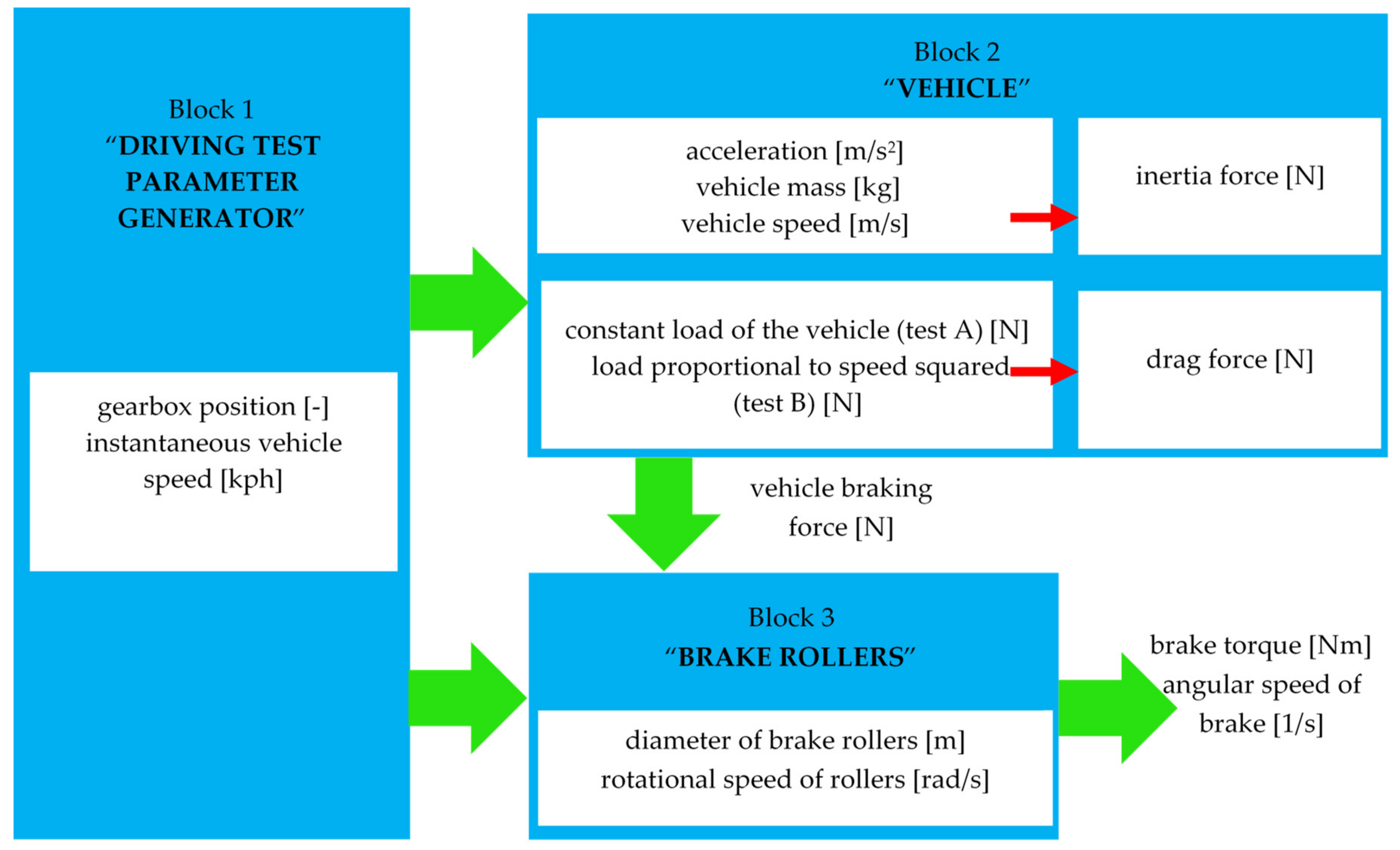
2.1. Determination of Dynamometer Requirements Based on Simulation of Driving Tests in SciLab

SciLab is a free program created for mathematical, engineering and data analysis purposes. SciLab contains hundreds of mathematical functions, has a high-level programming language that enables access to advanced data structures, 2D and 3D graphic functions. It can be used for engineering and scientific purposes based on mathematical operations and data analysis [93,94,95].
A simulation was built using the SciLab program, the purpose of which was to determine the requirements for the chassis dynamometer brake, with the possibility of testing vehicles up to 3.5 tons in road tests. Tests with the longest times and the largest loads during measurements were selected for the simulation:
  • CADCM150—Common Artemis Driving Cycle—Motor Medium with vMax = 150 kph
  • CADC150—Common Artemis Driving Cycle—Motor Highway with vMax = 150 kph
  • FTP75—EPA Federal Test Procedure—75 [0 … 1874] s at vMax = 56.7 mph = 91.25 kph
  • NEDC—New European Drive Cycle [0 … 1180] s = 4 × UDC + 1 × EUDC
  • WLTP—Worldwide Harmonized Light Vehicle Test Procedure—class 3 [0 … 1800] s at vMax = 131.3 kph.
Figure 1 presents a simulation diagram consisting of independent blocks responsible for: “Driving Test” that generates the course of the momentary speed of the vehicle over time on the basis of stored data compliant with standards of driving tests, “Vehicle” calculates the necessary loads acting on the vehicle during the test, “Brake Rollers”—based on the momentary values of vehicle speed and braking force on wheels fed to the module, the work parameters of the chassis dynamometer brake are calculated allowing the design parameter—the diameter of the brake rollers.
The “Vehicle” module reproduces the actual loads acting on the vehicle during the test, in accordance with the standards for conducting this type of test. Due to the fact that the available driving test data include the required courses of the vehicle speed in kilometres per hour, the first to convert in the module is the vehicle speed in the basic unit: m/s. In the calculation of the forces on the vehicle wheels, according to the vehicle, a component was used which enabled the determination of instantaneous acceleration of the vehicle. Calculations for the component force on the wheels resulting from the friction resistance included the following conversion factors, as required in the norm: Constant load value (F0 [N]), load value proportional to the vehicle speed (F1 [N/(kph)] and load value proportional to the vehicle speed squared (F2 [N/(kph)^2]) [96,97,98]. These forces are added together and forwarded to the next elements of the simulation. To generate graphs from driving test simulations, components (to workspace) were used to save the results of the simulation for later visualization.
The simulation block diagram developed in the SciLab program also includes a simulation module responsible for calculating the required torque and angular speed for the brake in the chassis dynamometer. In this case, these calculations include the diameters of the brake rollers adopted in the tests.
On top of the waveforms resulting from the driving test, additional lines were drawn that imaged the characteristic parameters of synchronous generators, which can be used as brakes in the chassis dynamometer. Due to the fact that changing the diameter of the brake rollers greatly affects the speed of the generators, two sets of generators with different operating speeds were selected to determine the parameters of the required device.
The momentary values of braking forces from vehicle dynamics ( Fm ) were calculated based on Equation (1):
Fm = m dv t dt   N
where: v t —The momentary speed of the vehicle in the test [m/s]; m —Vehicle calculation weight (455.0, 510.0, 570.0, …, 2270.0 kg) in the test.
The values of forces from motion resistance ( Fv ) were calculated according to relation (2):
Fv = a + b v t 2   N
where: v t —The momentary speed of the vehicle in the test [m/s]; a —Rolling resistance coefficient (3.8, 4.2, 4.4, …, 9.9 N); b —Aerodynamic resistance coefficient (0.0261, 0.0282, 0.0296, …, 0.0674 N/(km/h)2).
The momentary values of forces on the wheels ( F ) and the torque on the rollers ( M ) and the rotational speed of the rollers were calculated on the basis of the relationship (3), (4) and (5):
F = Fm + Fv   N
M = F R   N m
ω = v t R   rad s
where: F d ,   F o —Instantaneous force values on the rollers [N]; R —Radius of the brake rollers (0.217, 0.318, 0.504, 0.762 m); v t —The momentary speed of the vehicle in the test [m/s]
The maximum values of the torque on the rollers (Mmax) and the power received by the rollers (Pmax) were calculated on the basis of the relationship (6) and (7):
Mmax = max M   N m
Pmax = max M ω   W
In the case of brake roll diameters of 0.217 and 0.318 m, the graphs are marked with lines corresponding to the work parameters of generators operating at 3600 rpm: ECP 34-1S/2—Power 120 kVA red line; ECP 34-2S/2—Power 150 kVA green line; ECP34-1L/2—Power 174 kVA blue line; ECP 34-2L/2—Power 196 kVA light blue line.
For the diameter of the brake rollers 0.504 and 0.762 m, the graphs are marked with lines corresponding to the work parameters of generators operating at 1800 rpm: ECO38 1S4 A—Power 225 kVA red line; ECO38 2S4 A—Power 253 kVA green line; ECO38 3S4 A—Power 289 kVA blue line; ECO38 1L4 A—Power 319 kVA light blue line.

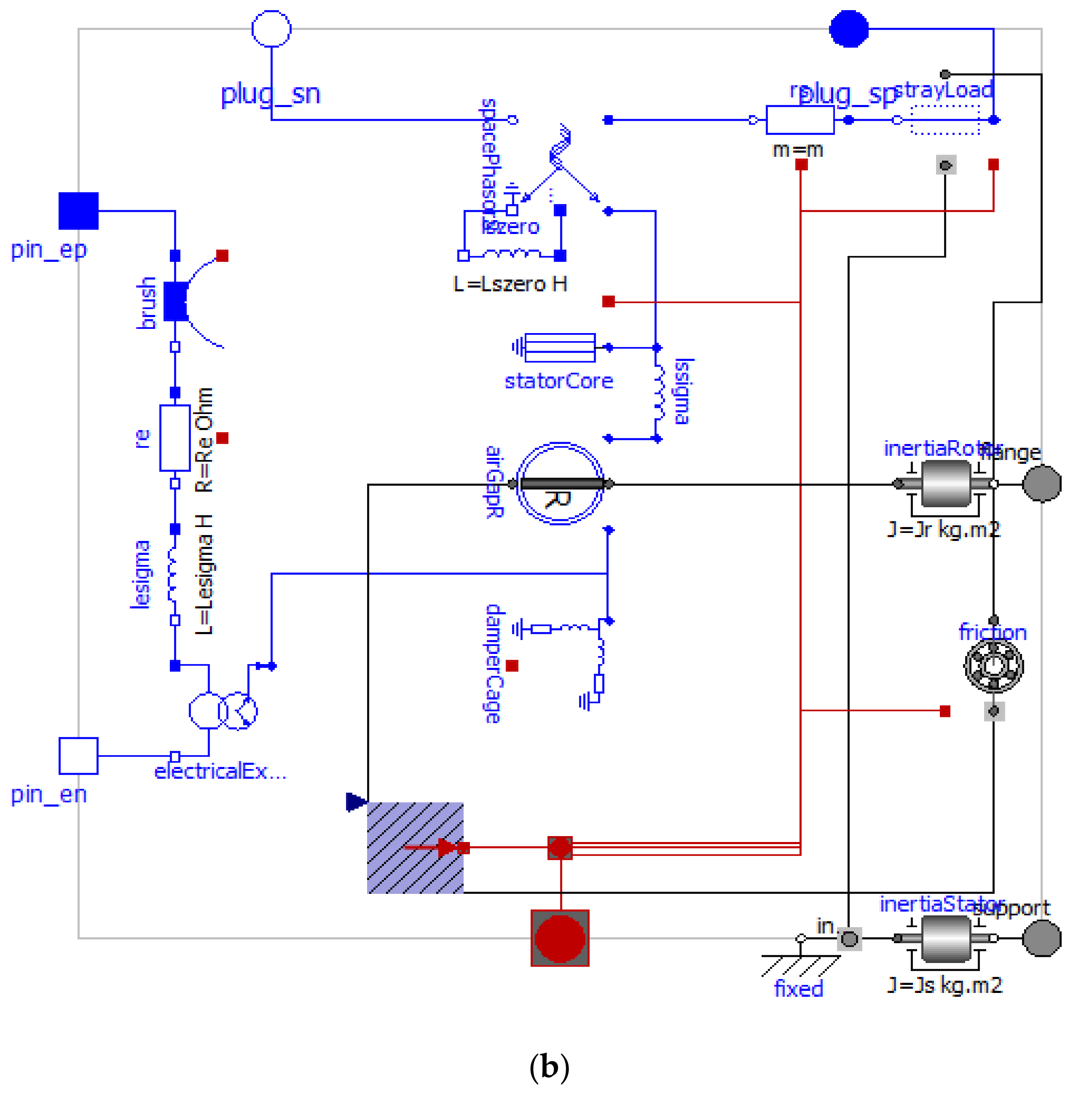
2.2. Simulation of the Braking Process for the Generator in the OpenModelica Program, in the Context of Driving Tests

OpenModelica is an open, interdisciplinary, comprehensive environment with graphic editors for modelling, compilation and construction of complex models and simulation control. The object-oriented modelling language Modelica is based on equations for industrial and academic applications. It is equipped with a large number of libraries dedicated to different domains [99,100,101].
A simulation has been developed in the OpenModelica program, the purpose of which is to obtain information on the possibility of using vehicles tested in braking of three-phase synchronous generators for braking (Figure 2a). In this simulation, the following components are responsible for the process of providing the required test parameters: TestW—Provides instant values of the angular speed of the brake rollers including the diameter of the rollers, TestM—Provides instantaneous values of the required braking torque. The element performing load simulations is a generator controlled by direct current excitation (“dcee”). A component (“pid”), simulating the PID controller with restrictions, was used to control the generator’s work parameters to create the necessary braking torque value.
The stator resistance and stray inductance is modelled directly in the stator phases, and then using a phase-space transformation and an AirGap model with a built-in rotor. The stray resistance and inductance of the rotor cage is modelled in two axes of the coordinate system mounted on the rotor. The electrical excitation is modelled by converting the excitation current and voltage into the spatial phases of the d axis. Machine models take into account the following loss effects: Heat losses in temperature-dependent stator winding resistances; heat losses depending on the temperature of the winding excitation; optionally, after switching on: Heat losses in cage resistances and temperature-dependent throttle; brush losses in the excitation circuit; losses due to friction; basic losses (only eddy current losses, no hysteresis losses); stray load losses. Figure 2b shows a schematic view of the simulation component of a three-phase synchronous generator included in the OpenModelica package [102].

3. Results

The simulation results obtained in the SciLab program were presented in the form of line and 3D graphs. Then, the simulation block diagrams made using the OpenModelica program, which referred to: determining the dynamometer requirements, calculating the instantaneous values of forces on the wheels of the vehicle during driving tests, calculating the instantaneous values of the torque and angular velocity in the dynamometer during tests and the loads of the tested brake were used to determine the possibility of using the generators tested in driving tests for braking.
In the presented simulation, the following parameters of the simulation tests were used: Vehicle calculation weight from 455 kg do 2270 kg, rolling resistance coefficients (3.8, 4.2, 4.4, …, 9.9 N), aerodynamic resistance coefficients (0.0261, 0.0282, 0.0296, …, 0.0674 N/(km/h)2).
These parameters are clearly defined in driving tests and are independent of vehicle operating parameters. A technically fit vehicle must only be able to achieve a course of instantaneous vehicle speed that matches the required test mileage during the test. At this stage, the purpose of which was to select the components of the chassis dynamometer, the operating parameters of the vehicles were not taken into account.

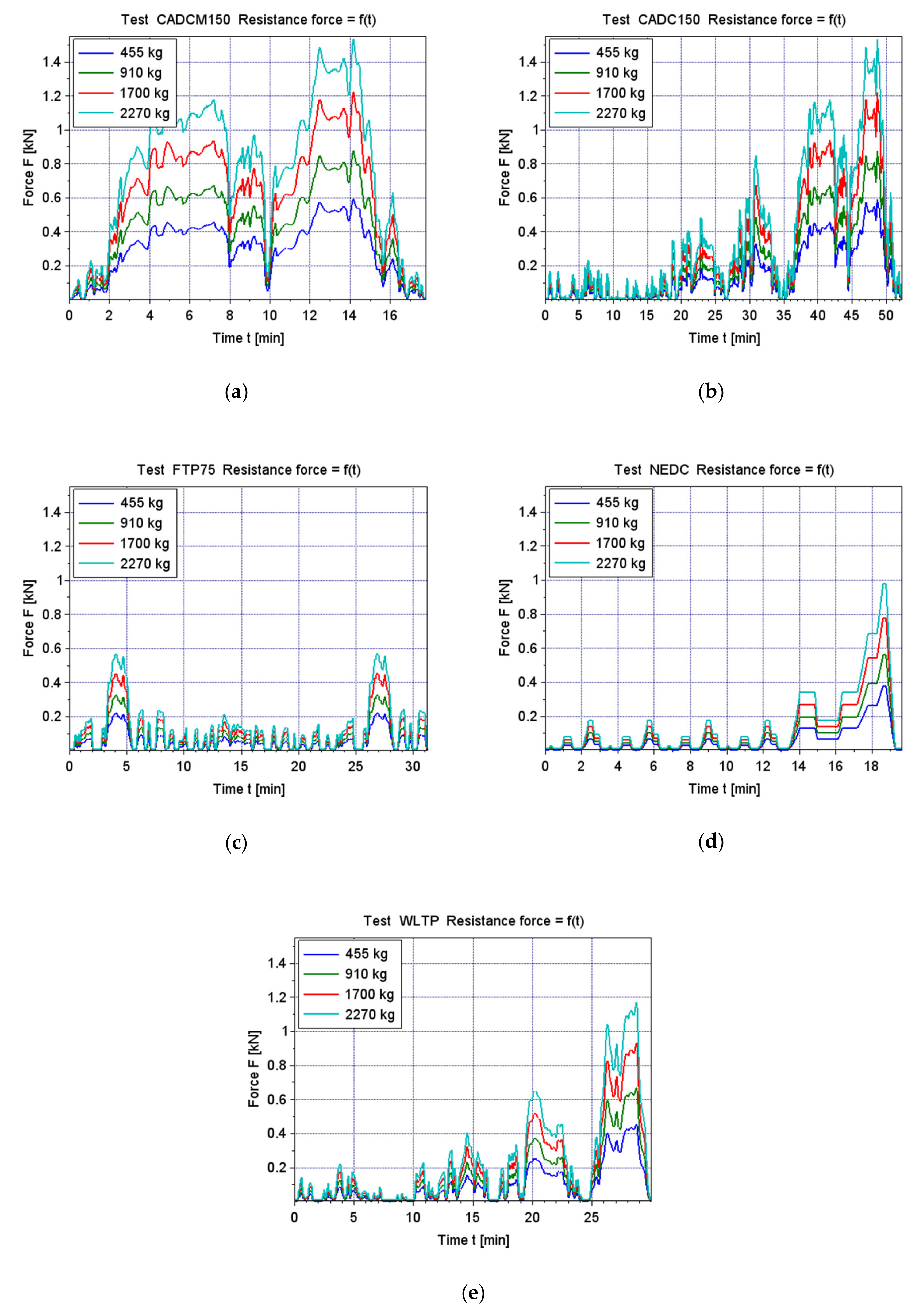
3.1. SciLab Simulation Results of Driving Tests for Various Braking Elements and Roller Sizes

The results of the simulation process for the adopted driving test were presented in the form of the course of the instantaneous value of the vehicle speed and the course of the instantaneous acceleration values acting on the vehicle. Then, the required loads in the vehicle movement were calculated using the vehicle mass classes, some examples of which are presented in the figure below (selected vehicle weight classes are included for the readability of the drawings) (Figure 3).
On the basis of the obtained results of individual simulations including the change of parameters: Mass of the tested vehicle and diameter of the brake rollers of the chassis dynamometer, a set of maximum values was drawn up: The required torque and the required power for the synchronous generators used (Figure 4).
Then, the waveforms of instantaneous angular velocity and braking torque values required for proper operation of the chassis dynamometer were generated. In this case, the largest allowable vehicle mass included in the standards (which generates the largest loads) and the change in the diameter of the brake rollers were taken into account. On top of the waveforms resulting from the driving test, additional lines were drawn that imaged the characteristic parameters of synchronous generators, which can be used as brakes in the chassis dynamometer. Due to the fact that changing the diameter of the brake rollers greatly affects the speed of the generators, two sets of generators with different operating speeds were selected to determine the parameters of the required device.

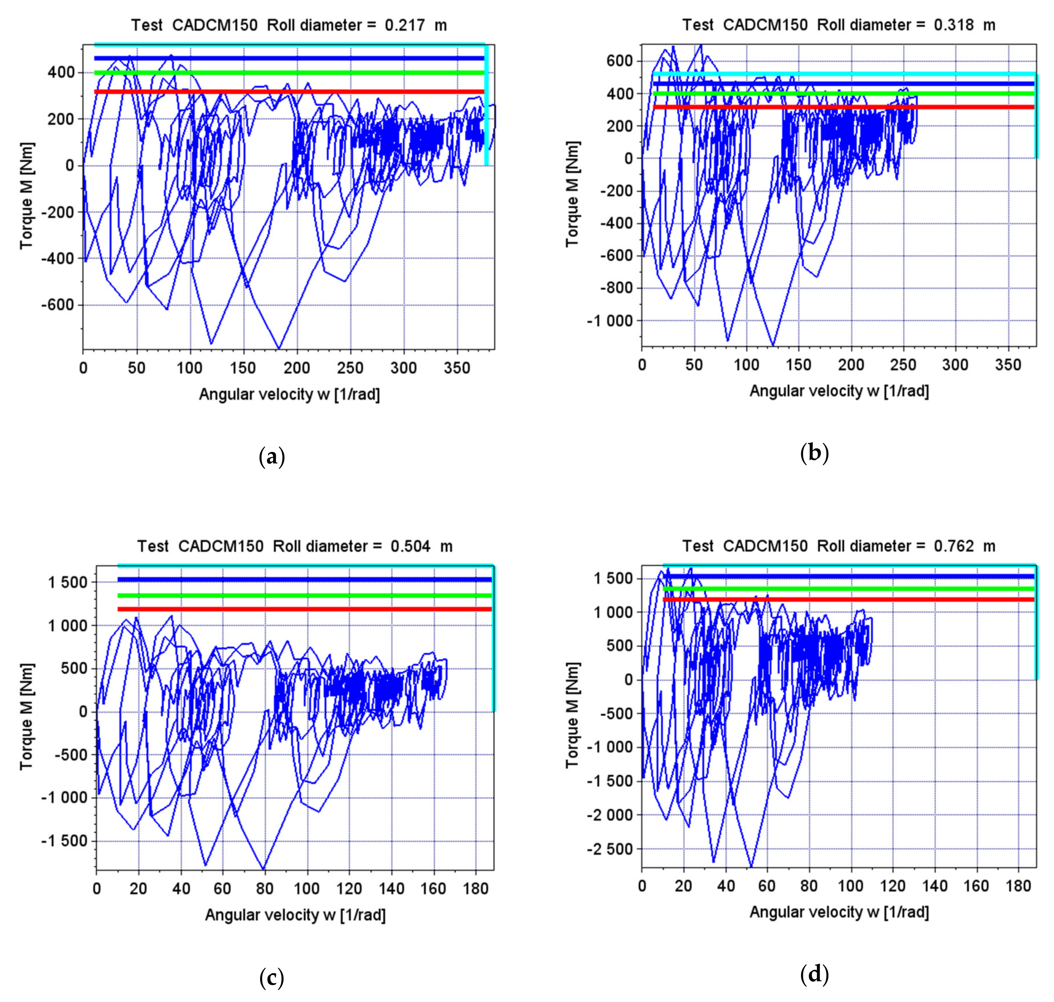
3.1.1. CADCM150 Driving Test

The results of the simulation process for the adopted CADCM150 test and including the above model were presented in waveforms of resistance force for selected vehicle masses in Figure 5. In the case of using a three-phase synchronous generator characterized by a maximum braking torque smaller than the maximum braking vehicle value resulting from the driving test, the waveform courses presented in the figures below exceed the values of restrictions arising from the lines drawn for individual generators. This situation potentially makes it impossible to carry out correct driving tests for the tested car (the vehicle load courses will not fit in the maximum defined deviations for the driving test).

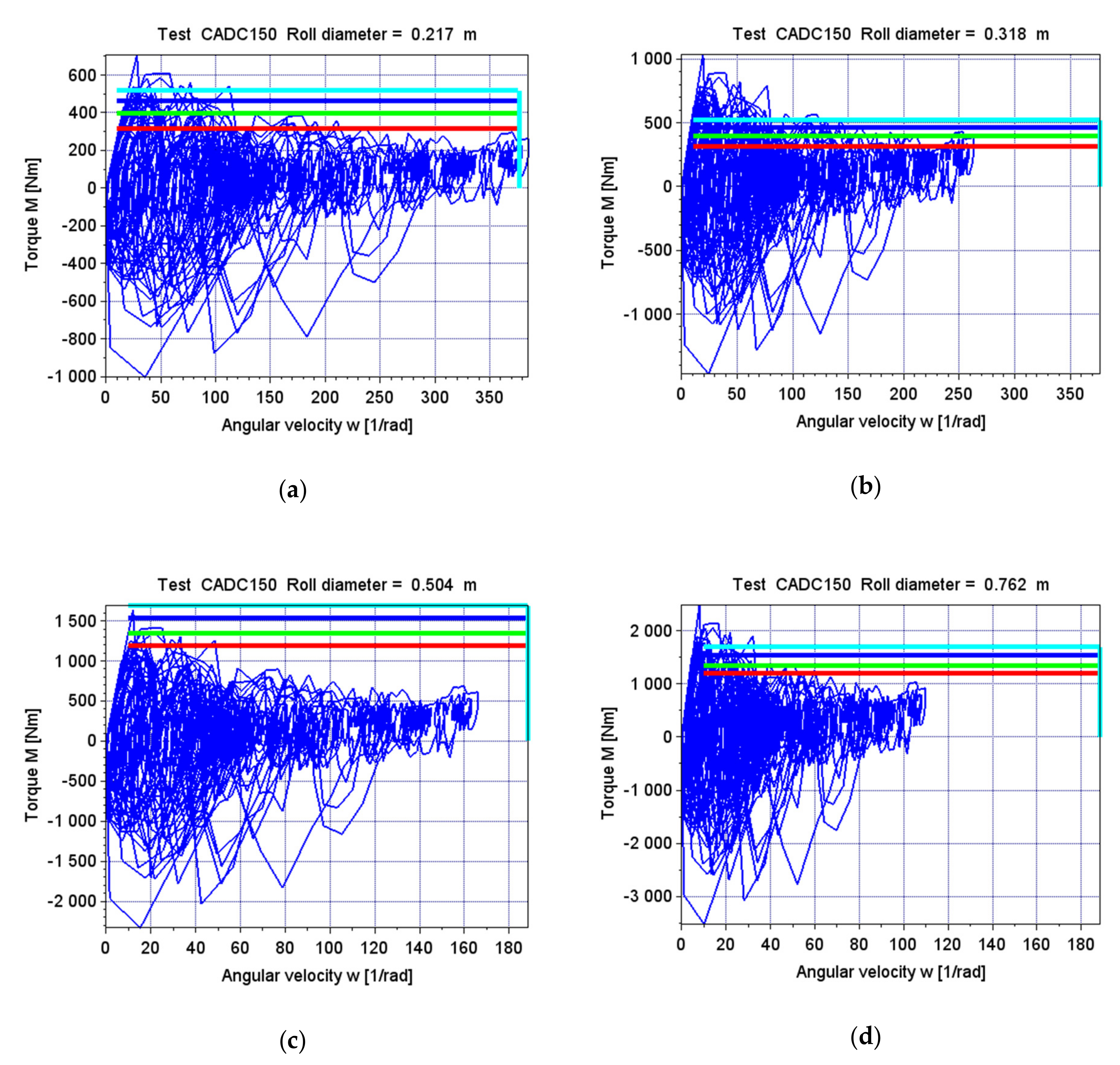
3.1.2. CADC150 Driving Test

In the case of the CADC150 driving test, just like in the previous test, after performing the necessary simulations, the maximum load values required to correctly conduct the driving test were collected in waveforms of instantaneous braking torque values, roller speed for assumed brake roller diameters. In addition, waveforms of instantaneous required angular velocity and torque values for the largest vehicle weight were also generated, taking into account the diameter of the rollers (Figure 6).

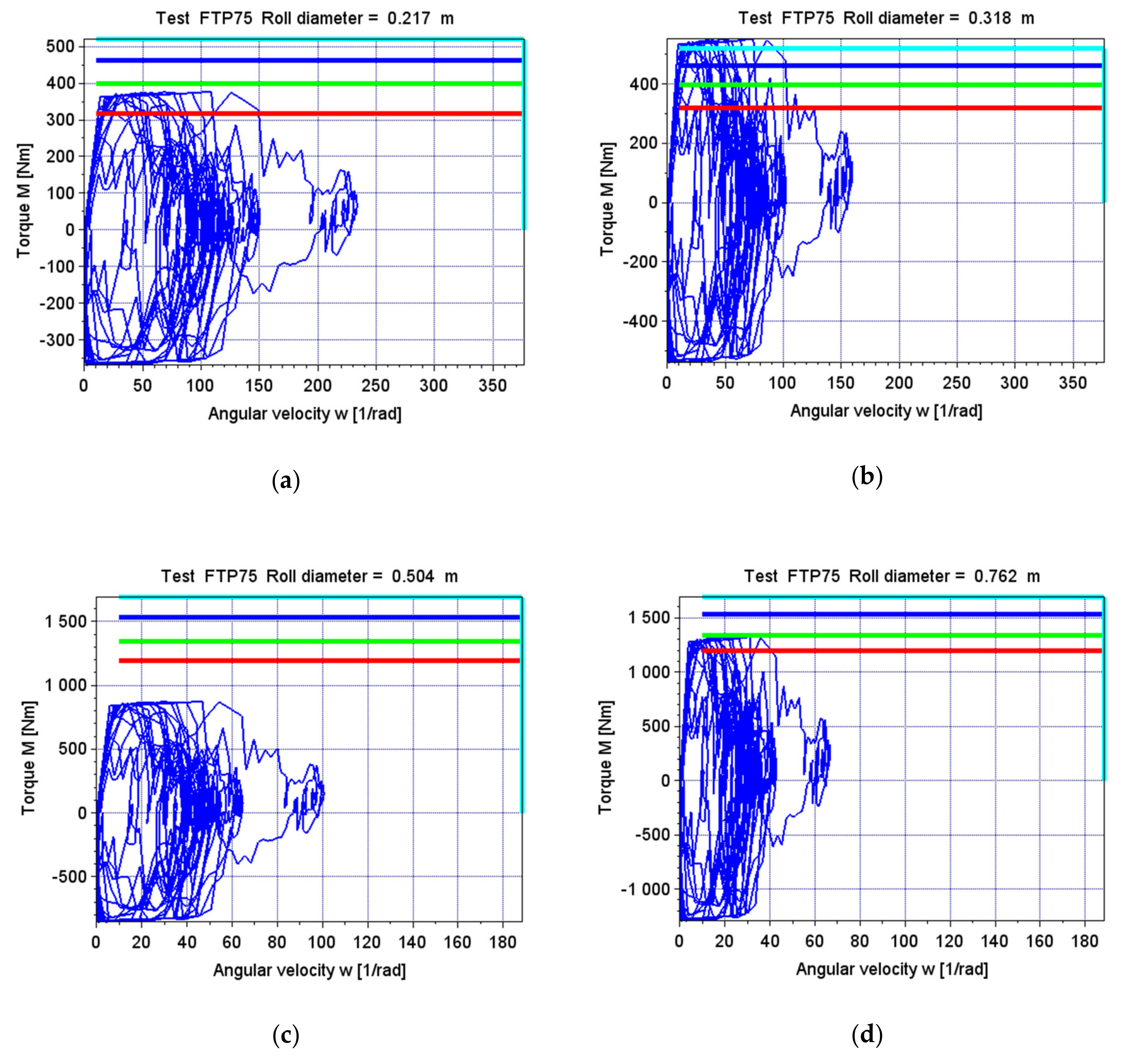
3.1.3. FTP75 Driving Test

The scheme for generating simulation results for the FTP75 travel test was identical for each type of driving test performed. Below (Figure 7) are shown the waveforms of instantaneous values of angular velocity and braking torque required for proper operation of the chassis dynamometer, taking into account the change in diameter of the brake rollers and lines characteristic for selected synchronous generators.

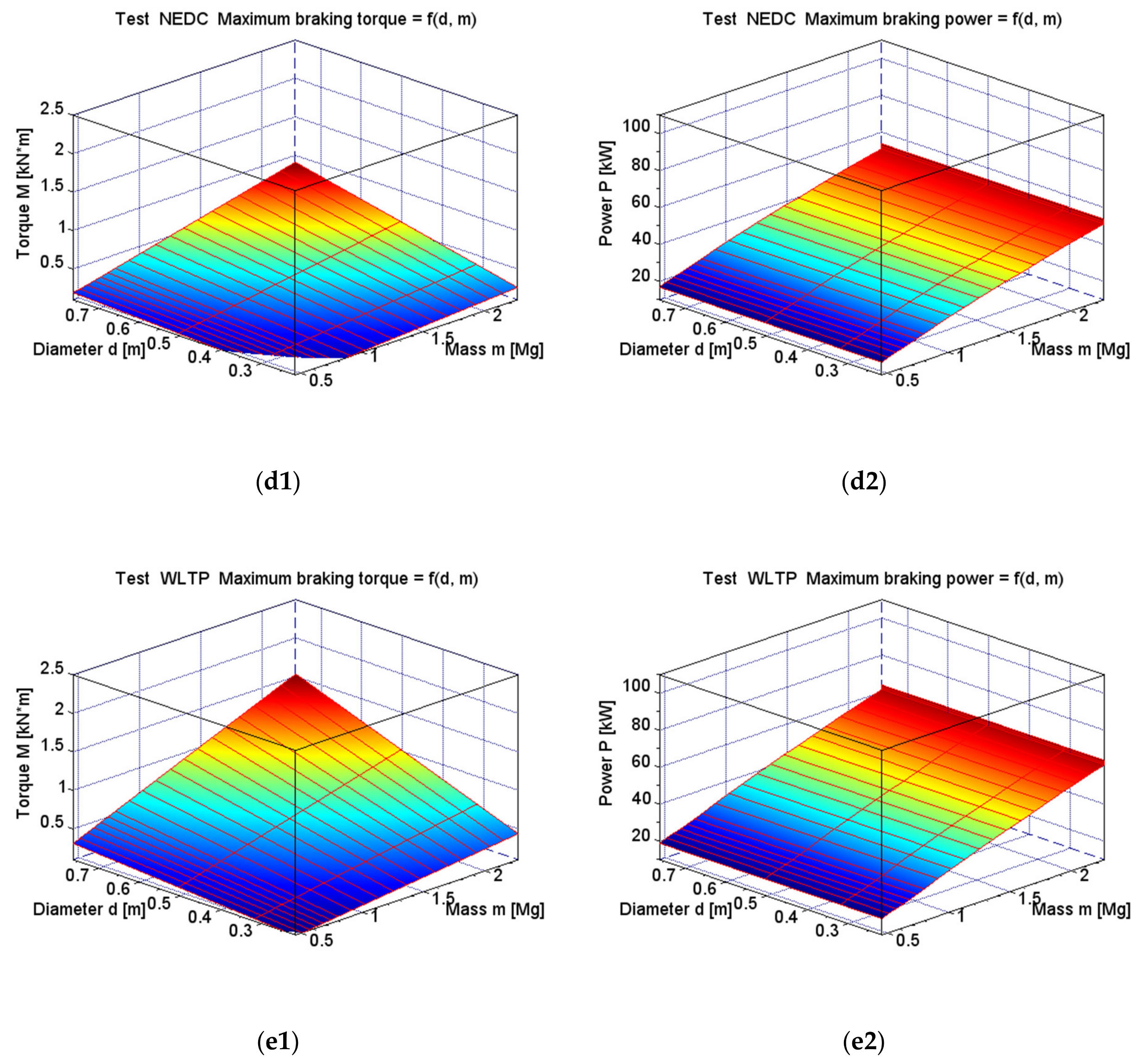
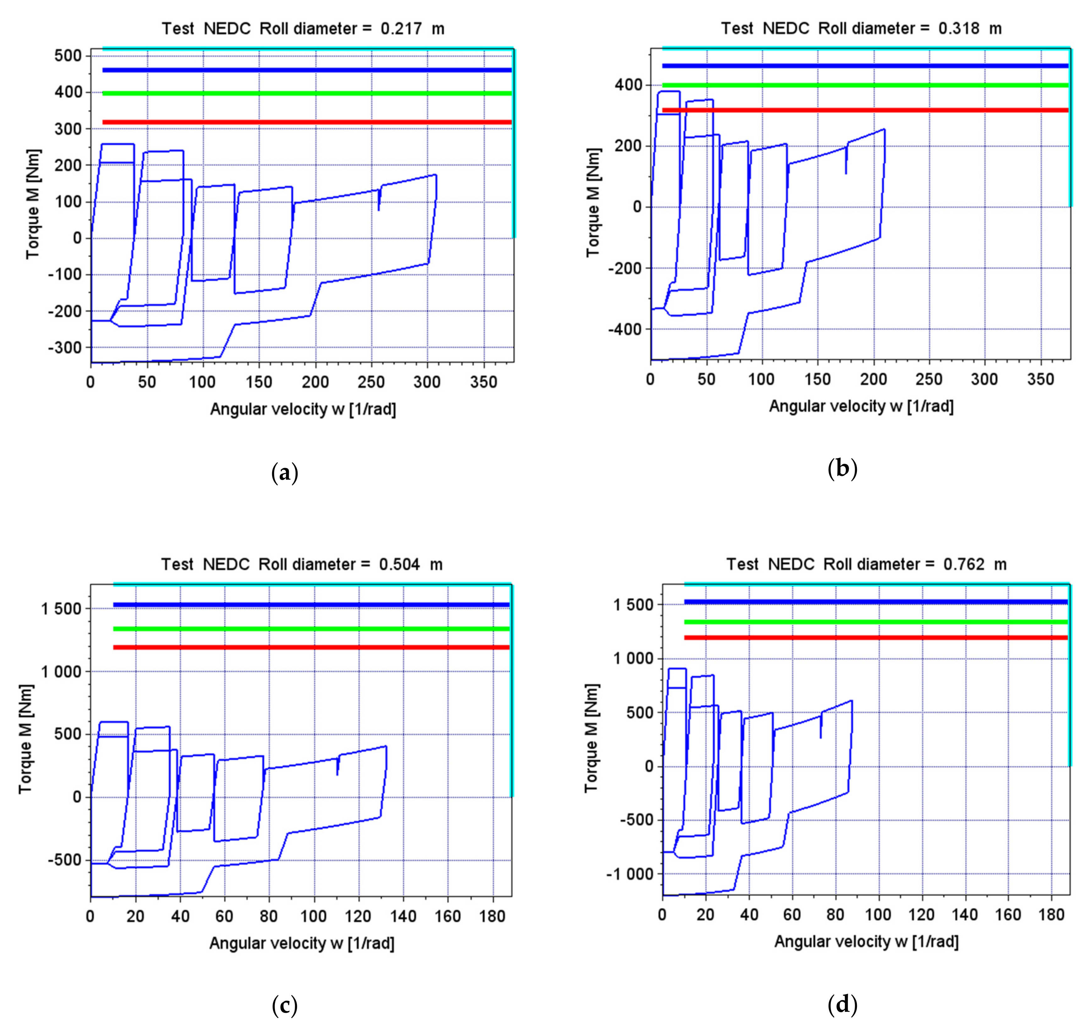
3.1.4. NEDC Driving Test

For the NEDC driving test, the simulation provided results that are presented below. The waveforms of the instantaneous torque and angular velocity values for the largest vehicle weight considered, including the diameter of the brake rollers, are shown in Figure 8.

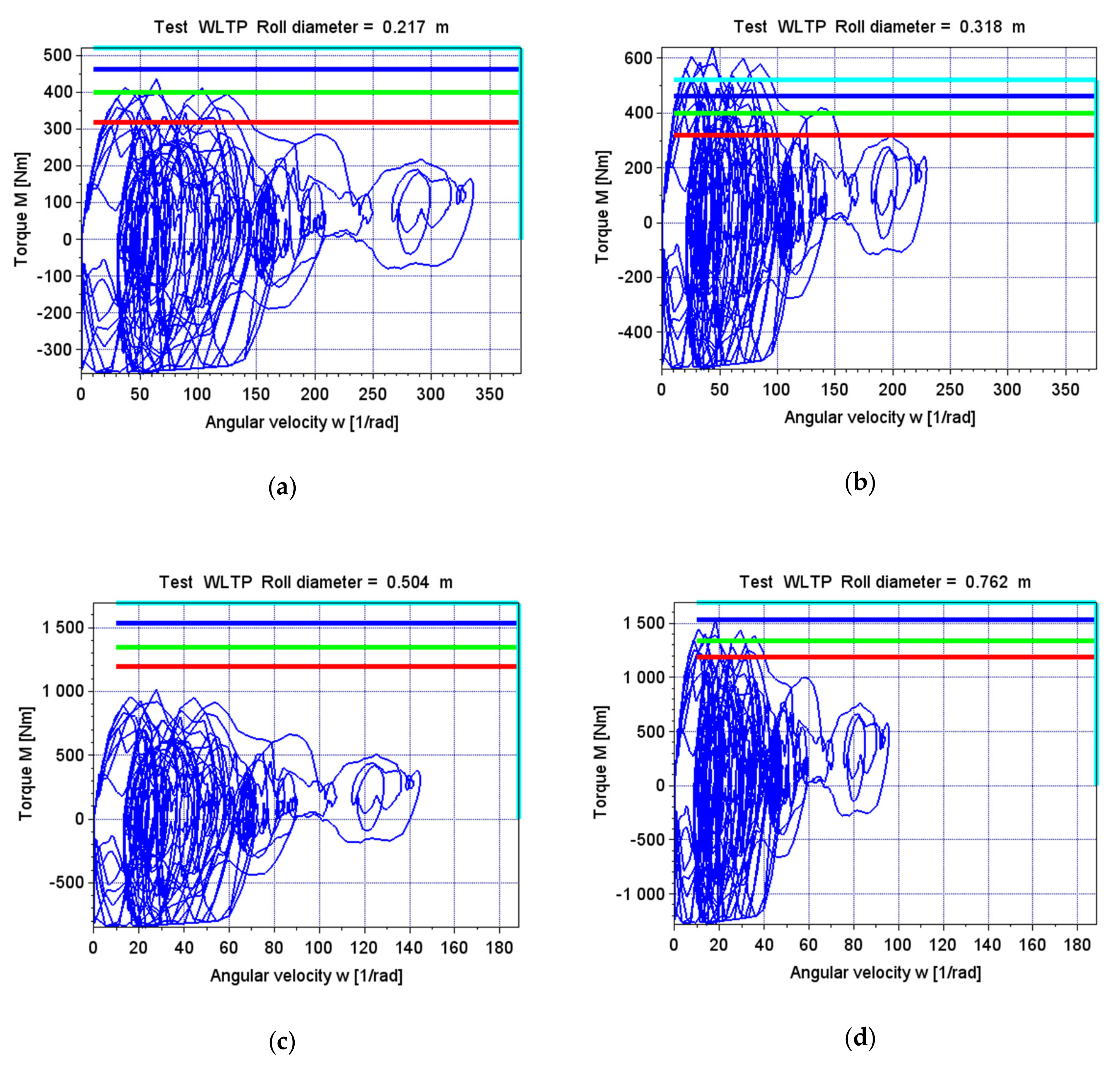
3.1.5. WLTP Driving Test

In the case of the WLTP travel test simulation, the results are presented in the form of graphs below. The instantaneous waveforms of braking torque and angular velocity for selected brake roller diameters are summarized in Figure 9. As in the previous examples, only the vehicle with the highest mass in the norm was included.

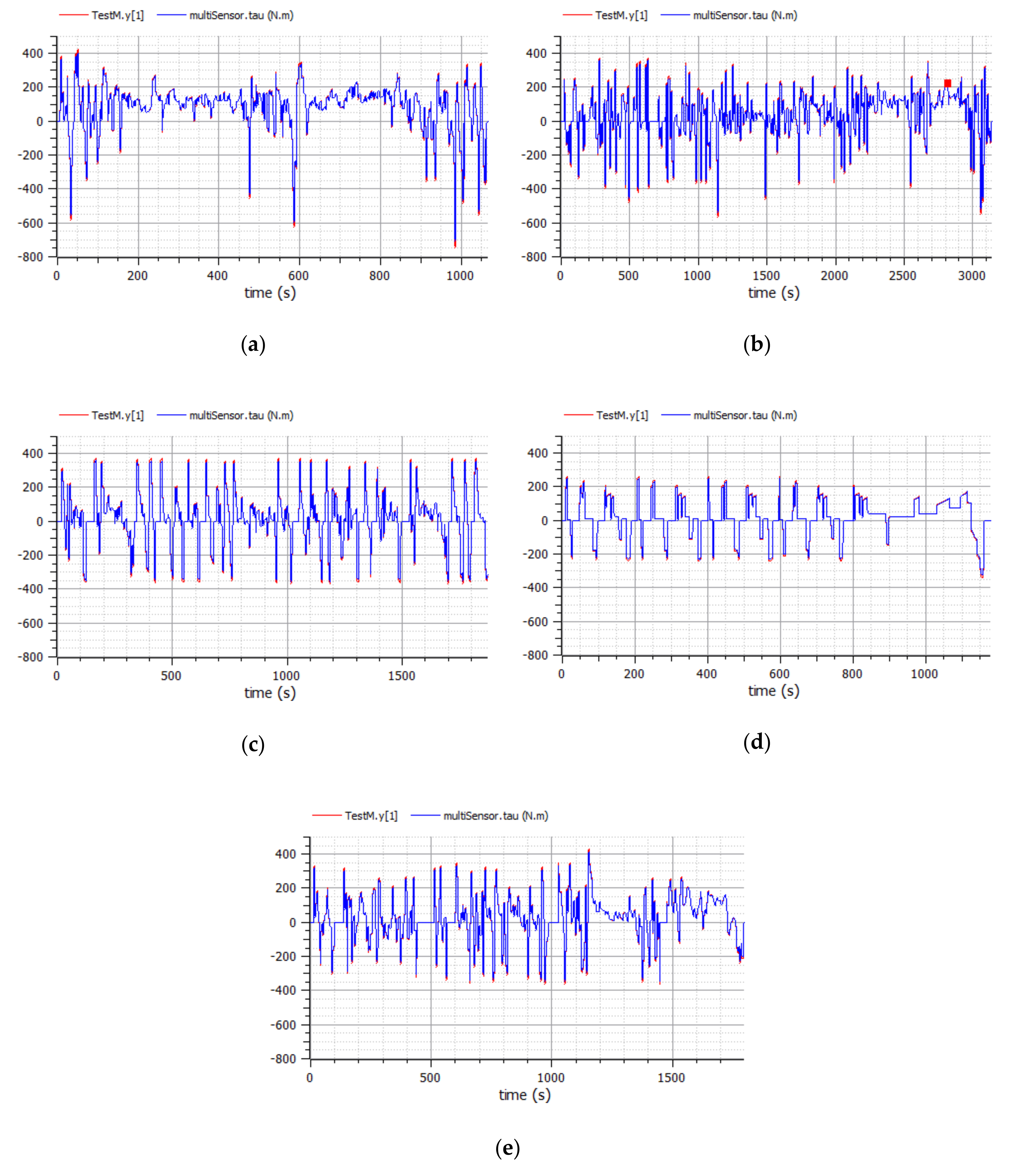
3.2. OpenModelica Simulation Results of the Braking Process for the Generator for Driving Tests

First, the results of the simulation of the generator’s operation were generated for the selected driving test in the form of a component containing the instantaneous value of rotational speed of the brake rollers. The figures below summarize the simulation results including the required braking torque and braking torque resulting from the actual simulation produced by the component of a three-phase synchronous generator (“dcee”).
The graphical results of computer simulations carried out for the tests are presented below: CADCM150, CAD150; FTP75, NEDC and WLTP (Figure 10).
The presented waveforms practically coincide with the values required for the test runs, which means that it is possible to use the generator for braking purposes in driving tests. In this case, it can be noticed that this component behaves like a generator loading the vehicle in the case of load simulation or as an electrical motor in the event of the vehicle decelerating.

4. Conclusions

The paper presents issues related to conducting driving tests in accordance with the accepted standards within the European Union and outside the EU (e.g., the USA).
  • Driving tests became the basis for building simulation models. However, to check the simulation position for the most common driving tests carried out worldwide (NEDC and WLTP), the following simulation input data were added to the set of simulation input data: CADCM150, CADC150, FTP75, which were characterized by the use of high speed of the vehicle movement during testing, which resulted in high demand of mechanical energy reception by the chassis dynamometer brake.
  • In order to determine the minimum required parameters of the element receiving energy from the vehicle in the aforementioned tests, a simulation was developed using the SciLab package. Based on the results obtained from the simulation processes, including the change in the driving test mode of the vehicle mass and the adopted diameter of the brake rollers, the minimum brake power value of 200 kVA at the rated speed of 3600 rpm was selected.
  • In the OpenModelica program, simulations of the component receiving mechanical power during the test were developed for: A generator with the option of controlling the excitation current. Based on the obtained results of the component, it can be concluded that the generators, due to the possibility of their work as an engine or generator, are better suited to a chassis dynamometer with dynamic tests of light vehicles up to 3.5 tons.
  • The analysis of the simulation results, including simulated driving tests, variable diameter of brake rollers and types of synchronous generators allowed to choose a generator that meets the requirements and is available on the market. Consequently, the simulation is the basis for further implementation work.
  • The special advantage of this type of electrical machine is the possibility of transferring the received energy during the driving test to the power grid, which reduces the amount of heat generated into the environment and irreversible energy losses.
  • The developed simulation constitutes a useful tool for initial research or planning of real experiments. It may be an element of a more comprehensive system or an independent system.
  • The authors in future research, presented in the manuscript of the tool, will expand on the results of experimental tests carried out on combustion engines powered by selected fuels and on simulations of work of other system components.

5. Discussion

The prepared simulation will be converted into software controlling the actual brake rollers. In the case of an actual test, the control application will perform the required load test for a vehicle with fixed mass values. During the drive test using the eOBD system, momentary operating values of the propulsion system will be collected from the vehicle control systems. Their analysis will be crucial in deciding whether or not to allow the vehicle to be put into service, and information on the errors of the said system, with an emphasis on emission-related errors.
Incorrect selection of the synchronous generator or incorrect operation of the synchronous generator and the control system for the excitation current of the synchronous generator leads to increased differences between the set driving test parameters resulting from the standards and the actual simulation parameters. Mileage errors can be caused by incorrect operation of the drive system (damage affecting engine power) and by incorrect operation of the brake rollers themselves.
The authors presented in the manuscript only the results of simulated driving tests and their analysis. It is planned to transfer the developed simulation to systems enabling real-time operation. The following environments are taken into account: FreeRTOS in the frame of software systems STM32CubeIDE, Matlab Simulink Real-Time.
In the developed simulation, the vehicle speed is the setpoint resulting from the specifics of the driving tests under consideration. At the simulation stage, no precise measurements of vehicle speed were made. However, the next steps in driving tests for the actual equipment and vehicles will use speed measurements using: Data acquisition from the vehicle’s OBD system, encoder sensor enabling measurement of the instantaneous value of the angle of rotation of the brake rollers. These sensors are characterized by a very high precision of the angle of rotation measurement and will be the basis for determining the vehicle speed. The signal from the vehicle’s ODB system, on the other hand, will compensate for the adverse effects on the speed measurement results, i.e., the deflection of the tyre on the brake rollers.
The authors use the Open Modelica environment in many threads of their research work. This is an open source environment for which all components are available in source form. The environment is not restricted in scientific implementation projects. The authors plan to use the library within the Open Modelica Modelica Device Drivers environment, Embedded Targets in future implementation work to build a brake roller control part. For this reason, the authors chose this environment. The authors have a license for the Matlab Simulink package; however, the license allows them to perform research and not implementation work.

Author Contributions

Conceptualization, K.T., O.O. and R.M., A.W.; methodology, K.T. and A.W.; software, K.T.; validation, K.T., O.O. and A.W., R.M.; investigation, K.T. and O.O.; resources, K.T. and A.W., R.M., O.O.; writing—Original draft preparation, K.T. and O.O.; writing—Review and editing, K.T.; Funding acquisition, O.O., A.W., K.T.; visualization, K.T. All authors have read and agreed to the published version of the manuscript.

Funding

The research was carried out under financial support obtained from the research subsidy of the Faculty of Engineering Management (WIZ) of Bialystok University of Technology. From the grant No. WI/WIZ-INZ/4/2019 (Olga Orynycz, Andrzej Wasiak). APC was funded by Institute of Mechanical Engineering money, SGGW.

Conflicts of Interest

The authors declare no conflict of interest. The funders had no role in the design of the study; in the collection, analyses, or interpretation of data; in the writing of the manuscript; or in the decision to publish the results.

References

  1. Capros, C.; Kannavou, M.; Evangelopoulou, S.; Petropoulos, A.; Siskos, P.; Tasios, N.; Zazias, G.; DeVita, A. Outlook of the EU energy system up to 2050: The case of scenarios prepared for European Commission’s “clean energy for all Europeans” package using the PRIMES model. Energy Strategy Rev. 2018, 22, 255–263. [Google Scholar] [CrossRef]
  2. Piwowar, A.; Dzikuć, M. Development of Renewable Energy Sources in the Context of Threats Resulting from Low-Altitude Emissions in Rural Areas in Poland: A Review. Energies 2019, 12, 3558. [Google Scholar] [CrossRef] [Green Version]
  3. Ng, C.W.; Tam, I.C.K.; Wu, D. System Modelling of Organic Rankine Cycle for Waste Energy Recovery System in Marine Applications. Energy Procedia 2019, 158, 1955–1961. [Google Scholar] [CrossRef]
  4. Aneke, M.; Agnew, B.; Underwood, C.; Wu, H.W.; Masheiti, S. Power generation from waste heat in a food processing application. Appl. Therm. Eng. 2012, 36, 171–180. [Google Scholar] [CrossRef]
  5. Production of Passenger Cars Worldwide from 1998 to 2018. Available online: https://www.statista.com/statistics/268739/production-of-passenger-cars-worldwide/ (accessed on 21 April 2020).
  6. Pettersson, P.; Johannesson, P.; Jacobson, B.; Bruzelius, F.; Fast, L.; Berglund, S. A statistical operating cycle description for prediction of road vehicles’ energy consumption. Transp. Res. Part D Transp. Environ. 2019, 73, 205–229. [Google Scholar] [CrossRef]
  7. Passenger Cars in the EU. Available online: https://ec.europa.eu/eurostat/ (accessed on 21 April 2020).
  8. Palkowski, K. Electric Car and Atmosphere Protection. Rocz. Ochr. Srodowiska Annu. Set Environ. Prot. 2016, 18, 628–639. [Google Scholar]
  9. Helmers, E.; Leitão, J.; Tietge, U.; Butler, T. CO2-equivalent emissions from European passenger vehicles in the years 1995–2015 based on real-world use: Assessing the climate benefit of the European “diesel boom”. Atmos. Environ. 2019, 198, 122–132. [Google Scholar] [CrossRef]
  10. Biernat, K. Perspectives for global development of biofuel technologies to 2050. Chemik 2012, 66, 1178–1189. [Google Scholar]
  11. Tucki, K.; Orynycz, O.; Świć, A.; Mitoraj-Wojtanek, M. The Development of Electromobility in Poland and EU States as a Tool for Management of CO2 Emissions. Energies 2019, 12, 2942. [Google Scholar] [CrossRef] [Green Version]
  12. Chłopek, Z.; Biedrzycki, J.; Lasocki, J.; Wójcik, P. Pollutant emissions from combustion engine of motor vehicle tested in driving cycles simulating real–world driving conditions. Zesz. Nauk. Inst. Pojazdów Politech. Warsz. 2013, 1, 67–76. [Google Scholar]
  13. Ambrozik, A.; Kurczyński, D.; Łagowski, P.; Warianek, M. The toxicity of combustion gas from the Fiat 1.3 Multijet engine operating following the load characteristics and fed with rape oil esters. Proc. Inst. Veh. 2016, 1, 23–36. [Google Scholar]
  14. Lee, T.; Shin, M.; Lee, B.; Chung, J.; Kim, D.; Keel, J.; Lee, S.; Kim, I.; Hong, Y. Rethinking NOx emission factors considering on-road driving with malfunctioning emission control systems: A case study of Korean Euro 4 light-duty diesel vehicles. Atmos. Environ. 2019, 202, 212–222. [Google Scholar] [CrossRef]
  15. Hooftman, N.; Messagie, M.; Van Mierlo, J.; Coosemans, T. A review of the European passenger car regulations—Real driving emissions vs local air quality. Renew. Sustain. Energy Rev. 2018, 86, 1–21. [Google Scholar] [CrossRef]
  16. Kuklinska, K.; Wolska, L.; Namiesnik, J. Air quality policy in the U.S. and the EU—A review. Atmos. Pollut. Res. 2015, 6, 129–137. [Google Scholar] [CrossRef]
  17. Regulation (EC) No 443/2009 of the European Parliament and of the Council of 23 April 2009 Setting Emission Performance Standards for New Passenger Cars as Part of the Community’s Integrated Approach to Reduce CO2 Emissions from Light-Duty Vehicles (Text with EEA Relevance). Available online: https://eur-lex.europa.eu/ (accessed on 21 April 2020).
  18. Bocheńki, C. Biofuels in agriculture. Agric. Eng. 2008, 1, 23–26. [Google Scholar]
  19. Mendoza-Villafuerte, P.; Suarez-Bertoa, R.; Giechaskiel, B.; Riccobono, F.; Bulgheroni, C.; Astorga, C.; Perujo, A. NOx, NH3, N2O and PN real driving emissions from a Euro VI heavy-duty vehicle. Impact of regulatory on-road test conditions on emissions. Sci. Total Environ. 2017, 609, 546–555. [Google Scholar] [CrossRef]
  20. Triantafyllopoulos, G.; Dimaratos, A.; Ntziachristos, L.; Bernard, Y.; Dornoff, J.; Samaras, Z. A study on the CO2 and NOx emissions performance of Euro 6 diesel vehicles under various chassis dynamometer and on-road conditions including latest regulatory provisions. Sci. Total Environ. 2019, 666, 337–346. [Google Scholar] [CrossRef]
  21. Grigoratos, T.; Fontaras, G.; Giechaskiel, B.; Zacharof, N. Real world emissions performance of heavy-duty Euro VI diesel vehicles. Atmos. Environ. 2019, 201, 348–359. [Google Scholar] [CrossRef]
  22. Terzis, A.; Kirsch, M.; Vaikuntanathan, V.; Geppert, A.; Lamanna, G.; Weigand, B. Splashing characteristics of diesel exhaust fluid (AdBlue) droplets impacting on urea-water solution films. Exp. Therm. Fluid Sci. 2019, 102, 152–162. [Google Scholar] [CrossRef]
  23. Tucki, K.; Mruk, R.; Orynycz, O.; Wasiak, A.; Botwińska, K.; Gola, A. Simulation of the Operation of a Spark Ignition Engine Fueled with Various Biofuels and Its Contribution to Technology Management. Sustainability 2019, 11, 2799. [Google Scholar] [CrossRef] [Green Version]
  24. Xiao, H.; Guo, F.; Li, S.; Wang, R.; Yang, X. Combustion performance and emission characteristics of a diesel engine burning biodiesel blended with n-butanol. Fuel 2019, 258, 115887. [Google Scholar] [CrossRef]
  25. Huang, Y.; Ng, E.C.Y.; Yam, Y.S.; Lee, C.K.C.; Surawski, N.C.; Mok, W.C.; Organ, B.; Zhou, J.L.; Chan, E.F.C. Impact of potential engine malfunctions on fuel consumption and gaseous emissions of a Euro VI diesel truck. Energy Convers. Manag. 2019, 184, 521–529. [Google Scholar] [CrossRef]
  26. Merkisz, J.; Pielecha, I.; Pielecha, J.; Brudnicki, K. On-Road Exhaust Emissions from Passenger Cars Fitted with a Start-Stop System. Arch. Transp. 2011, 23, 37–46. [Google Scholar] [CrossRef] [Green Version]
  27. Dobrzyńska, E.; Szewczyńska, M.; Pośniak, M.; Szczotka, A.; Puchałka, B.; Woodburn, J. Exhaust emissions from diesel engines fueled by different blends with the addition of nanomodifiers and hydrotreated vegetable oil HVO. Environ. Pollut. 2020, 259, 113772. [Google Scholar] [CrossRef] [PubMed]
  28. Odziemkowska, M.; Czarnocka, J.; Frankiewicz, A.; Szewczyńska, M.; Lankoff, A.; Gromadzka-Ostrowska, J.; Mruk, R. Chemical characterization of exhaust gases from compression ignition engine fuelled with various biofuels. Pol. J. Environ. Stud. 2017, 26, 1183–1190. [Google Scholar] [CrossRef]
  29. O’Driscoll, R.; Stettler, M.E.J.; Molden, N.; Oxley, T.; ApSimon, H.M. Real world CO2 and NOx emissions from 149 Euro 5 and 6 diesel, gasoline and hybrid passenger cars. Sci. Total Environ. 2018, 621, 282–290. [Google Scholar] [CrossRef]
  30. Bielaczyc, P.; Szczotka, A.; Pajdowski, P.; Woodburn, J. The potential of current European light duty LPG-fuelled vehicles to meet Euro 6 requirement. Combust. Engines 2015, 162, 874–880. [Google Scholar]
  31. Millo, F.; Giacominetto, P.F.; Bernardi, M.G. Analysis of different exhaust gas recirculation architectures for passenger car Diesel engines. Appl. Energy 2012, 98, 79–91. [Google Scholar] [CrossRef]
  32. Lozhkin, V.; Lozhkina, O.; Dobromirov, V. A study of air pollution by exhaust gases from cars in well courtyards of Saint Petersburg. Transp. Res. Procedia 2018, 36, 453–458. [Google Scholar] [CrossRef]
  33. Kilicarslan, A.; Qatu, M. Exhaust Gas Analysis of an Eight Cylinder Gasoline Engine Based on Engine Speed. Energy Procedia 2017, 110, 459–464. [Google Scholar] [CrossRef]
  34. Den Tonkelaar, W.A.M. CAR Smog: System for on-line extrapolation from hourly measurements to concentrations along standard roads within cities. Sci. Total Environ. 1996, 189–190, 423–429. [Google Scholar] [CrossRef]
  35. Frankowski, J. Attention: Smog alert! Citizen engagement for clean air and its consequences for fuel poverty in Poland. Energy Build. 2019, 207, 109525. [Google Scholar] [CrossRef]
  36. Gao, J.; Chen, H.; Li, Y.; Chen, J.; Zhang, Y.; Dave, K.; Huang, Y. Fuel consumption and exhaust emissions of diesel vehicles in worldwide harmonized light vehicles test cycles and their sensitivities to eco-driving factors. Energy Convers. Manag. 2019, 196, 605–613. [Google Scholar] [CrossRef]
  37. Mansour, C.; Nader, W.B.; Breque, F.; Haddad, M.; Nemer, M. Assessing additional fuel consumption from cabin thermal comfort and auxiliary needs on the worldwide harmonized light vehicles test cycle. Transp. Res. Part D Transp. Environ. 2018, 62, 139–151. [Google Scholar] [CrossRef]
  38. Gużda, A.; Szmolke, N. Variability of selected air parameters in the premises containing a car dynamometer. Autobusy 2017, 6, 208. [Google Scholar]
  39. Chen, L.; Wang, Z.; Liu, S.; Qu, L. Using a chassis dynamometer to determine the influencing factors for the emissions of Euro VI vehicles. Transp. Res. Part D Transp. Environ. 2018, 65, 564–573. [Google Scholar] [CrossRef]
  40. Li, T.; Chen, X.; Yan, Z. Comparison of fine particles emissions of light-duty gasoline vehicles from chassis dynamometer tests and on-road measurements. Atmos. Environ. 2013, 68, 82–91. [Google Scholar] [CrossRef]
  41. Gołębiewski, W.; Prajwowski, K. The use of road dynamometer to determine engine operating parameters. Autobusy 2014, 6, 100–104. [Google Scholar]
  42. Ruan, D.; Xie, H.; Song, K.; Zhang, G. Adaptive Speed Control based on Disturbance Compensation for Engine-Dynamometer System. IFAC-PapersOnLine 2019, 52, 642–647. [Google Scholar] [CrossRef]
  43. Kęder, M.; Grzeszczyk, R.; Merkisz, J.; Fuć, P.; Lijewski, P. Design of a new engine dynamometer test stand for driving cycle simulation. J. KONES 2014, 21, 217–224. [Google Scholar] [CrossRef]
  44. Huertas, J.I.; Giraldo, M.; Quirama, L.F.; Díaz, J. Driving Cycles Based on Fuel Consumption. Energies 2018, 11, 3064. [Google Scholar] [CrossRef] [Green Version]
  45. Pavlovic, J.; Ciuffo, B.; Fontaras, G.; Valverde, V.; Marotta, A. How much difference in type-approval CO2 emissions from passenger cars in Europe can be expected from changing to the new test procedure (NEDC vs. WLTP)? Transp. Res. Part A Policy Pract. 2018, 111, 136–147. [Google Scholar] [CrossRef]
  46. Mazer, M.; Hatschbach, L.; Dos Santos, I.; Silveira, J.; Garlet, R.A.; Martins, M.E.S.; Nora, M.D. Comparison between the WLTC and the FTP-75 Driving Cycles Applied to a 1.4 L Light-Duty Vehicle Running on Ethanol. Available online: https://www.sae.org/publications/technical-papers/content/2019-36-0144/ (accessed on 21 April 2020).
  47. Committee of Inquiry into Emission Measurements in the Automotive Sector. Working Document No. 12. on the Inquiry into Emission Measurements in the Automotive Sector—Appendix E: Glossary. Available online: https://www.europarl.europa.eu/doceo/document/EMIS-DT-594082_EN.pdf?redirect (accessed on 21 April 2020).
  48. Żółtowski, A. Comparison of pollutant emissions test cycles for ic engines. J. KONES Powertrain Transp. 2007, 14, 591–598. [Google Scholar]
  49. Tucki, K.; Mruk, R.; Baczyk, A.; Botwinska, B.; Wozniak, K. Analysis of the Exhaust Gas Emission Level from a Diesel Engine with Using Computer Simulation. Rocz. Ochr. Srodowiska 2018, 20, 1095–1112. [Google Scholar]
  50. Król, E. Comparison of emissions of electric and diesel vehicles. Napędy Sterow. 2017, 19, 140–143. [Google Scholar]
  51. Suchecki, A.; Nowakowski, J. Research during the approval process on a chassis and engine dynamometer. Badania 2015, 12, 1459–1463. [Google Scholar]
  52. Łączyński, J. Type aprval tests of the car designed for the transport of disable persons. Autobusy 2013, 3, 749–759. [Google Scholar]
  53. Wu, T.; Han, X.; Zheng, M.M.; Ou, X.; Sun, H.; Zhang, X. Impact factors of the real-world fuel consumption rate of light duty vehicles in China. Energy 2020, 190, 116388. [Google Scholar] [CrossRef]
  54. Karagöz, Y. Analysis of the impact of gasoline, biogas and biogas + hydrogen fuels on emissions and vehicle performance in the WLTC and NEDC. Int. J. Hydrogen Energy 2019, 44, 31621–31632. [Google Scholar] [CrossRef]
  55. Emission Standards. Summary of Worldwide Engine and Vehicle Emission Standards. Available online: https://dieselnet.com/standards/#eu (accessed on 21 April 2020).
  56. Franco, V.; Delgado, O.; Muncrief, R. Heavy-Duty Vehicle Fuel-Efficiency Simulation: A Comparison of Us and Eu Tools. Available online: https://theicct.org/sites/default/files/publications/ICCT_GEM-VECTO-comparison_20150511.pdf (accessed on 21 April 2020).
  57. Kocsis, L.; Iclodean, C.D.; Gaspar, F.; Burnete, N.V. Comparison of international vehicle testing cycles using simulation. Rom. J. Tech. Sci. 2018, 1, 25–35. [Google Scholar]
  58. Pavlovic, J.; Marotta, A.; Ciuffo, B. CO2 emissions and energy demands of vehicles tested under the NEDC and the new WLTP type approval test procedures. Appl. Energy 2016, 177, 661–670. [Google Scholar] [CrossRef]
  59. Dimaratos, A.; Tsokolis, D.; Fontaras, G.; Tsiakmakis, S.; Ciuffo, B.; Samaras, Z. Comparative Evaluation of the Effect of Various Technologies on Light-duty Vehicle CO2 Emissions over NEDC and WLTP. Transp. Res. Procedia 2016, 14, 3169–3178. [Google Scholar] [CrossRef] [Green Version]
  60. Massaguer, E.; Massaguer, A.; Pujol, T.; Comamala, M.; Montoro, L.; Gonzalez, J.R. Fuel economy analysis under a WLTP cycle on a mid-size vehicle equipped with a thermoelectric energy recovery system. Energy 2019, 179, 306–314. [Google Scholar] [CrossRef]
  61. Kim, J.; Choi, K.; Myung, C.L.; Lee, Y.; Park, S. Comparative investigation of regulated emissions and nano-particle characteristics of light duty vehicles using various fuels for the FTP-75 and the NEDC mode. Fuel 2013, 106, 335–343. [Google Scholar] [CrossRef]
  62. Choi, Y.; Lee, J.; Jang, J.; Park, S. Effects of fuel-injection systems on particle emission characteristics of gasoline vehicles. Atmos. Environ. 2019, 2017, 116941. [Google Scholar] [CrossRef]
  63. Roso, V.R.; Santos, N.D.S.A.; Valle, R.M.; Alvarez, C.E.C.; Monsalve-Serrano, J.; García, A. Evaluation of a stratified prechamber ignition concept for vehicular applications in real world and standardized driving cycles. Appl. Energy 2019, 254, 113691. [Google Scholar] [CrossRef]
  64. Puškár, M.; Jahnátek, A.; Kádárová, J.; Šoltésová, M.; Kovanič, L.; Krivosudská, J. Environmental study focused on the suitability of vehicle certifications using the new European driving cycle (NEDC) with regard to the affair “dieselgate” and the risks of NOx emissions in urban destinations. Air Qual. Atmos. Health 2019, 12, 251–257. [Google Scholar] [CrossRef]
  65. Shim, B.J.; Park, K.S.; Koo, J.M.; Jin, S.H. Work and speed based engine operation condition analysis for new European driving cycle (NEDC). J. Mech. Sci. Technol. 2014, 28, 755–761. [Google Scholar] [CrossRef]
  66. Pavlovic, J.; Fontaras, G.; Ktistakis, M.; Anagnostopoulos, K.; Komnos, D.; Ciuffo, B.; Clairotte, M.; Valverde, V. Understanding the origins and variability of the fuel consumption gap: Lessons learned from laboratory tests and a real-driving campaign. Environ. Sci. Eur. 2020, 32, 53. [Google Scholar] [CrossRef] [Green Version]
  67. EU: Light-Duty: New European Driving Cycle. Available online: https://www.transportpolicy.net/standard/eu-light-duty-new-european-driving-cycle/ (accessed on 21 April 2020).
  68. Degraeuwe, B.; Weiss, M. Does the New European Driving Cycle (NEDC) really fail to capture the NOX emissions of diesel cars in Europe? Environ. Pollut. 2017, 222, 234–241. [Google Scholar] [CrossRef] [PubMed]
  69. Bielaczyc, P.; Woodburn, J. Trends in Automotive Emission Legislation: Impact on LD Engine Development, Fuels, Lubricants and Test Methods: A Global View, with a Focus on WLTP and RDE Regulations. Emiss. Control Sci. Technol. 2019, 5, 86–98. [Google Scholar] [CrossRef] [Green Version]
  70. Pfaffelhuber, K.; Uhl, F. Engine Encapsulations for Fewer Cold Starts. ATZ Worldw. 2015, 117, 20–23. [Google Scholar] [CrossRef]
  71. Singh, T.; Balzer, D.; Leertouwer, K.; Wise, J. WLTP Regulations and Advanced Recuperation Strategies. ATZ Worldw. 2018, 120, 50–53. [Google Scholar] [CrossRef]
  72. From NEDC to WLTP: Effect on the Type-Approval CO2 Emissions of Light-Duty Vehicles. Available online: https://ec.europa.eu/jrc/en/publication/eur-scientific-and-technical-research-reports/nedc-wltp-effect-type-approval-co2-emissions-light-duty-vehicles (accessed on 21 April 2020).
  73. Commission Regulation (EU) 2018/1832 of 5 November 2018 amending Directive 2007/46/EC of the European Parliament and of the Council, Commission Regulation (EC) No 692/2008 and Commission Regulation (EU) 2017/1151 for the Purpose of Improving the Emission Type Approval Tests and Procedures for Light Passenger and Commercial Vehicles, Including Those for In-Service Conformity and Real-Driving Emissions and Introducing Devices for Monitoring the Consumption of Fuel and Electric Energy (Text with EEA Relevance.) C/2018/6984. Available online: https://eur-lex.europa.eu/legal-content/EN/TXT/?uri=CELEX%3A32018R1832 (accessed on 21 April 2020).
  74. Tsiakmakis, S.; Fontaras, G.; Anagnostopoulos, K.; Ciuffo, B.; Pavlovic, J.; Marotta, A. A simulation based approach for quantifying CO2 emissions of light duty vehicle fleets. A case study on WLTP introduction. Transp. Res. Procedia 2017, 25, 3898–3908. [Google Scholar] [CrossRef]
  75. United States Environmental Protection Agency. Vehicle and Fuel Emissions Testing. Available online: https://www.epa.gov/vehicle-and-fuel-emissions-testing/dynamometer-drive-schedules (accessed on 21 April 2020).
  76. Myung, C.L.; Jang, W.; Kwon, S.; Ko, J.; Jin, D.; Park, S. Evaluation of the real-time de-NOx performance characteristics of a LNT-equipped Euro-6 diesel passenger car with various vehicle emissions certification cycles. Energy 2017, 132, 356–369. [Google Scholar] [CrossRef]
  77. Wi, H.; Park, J. Analyzing uncertainty in evaluation of vehicle fuel economy using FTP-75. Int. J. Automot. Technol. 2013, 14, 471–477. [Google Scholar] [CrossRef]
  78. Chan, T.W.; Meloche, E.; Kubsh, J.; Brezny, R. Black Carbon Emissions in Gasoline Exhaust and a Reduction Alternative with a Gasoline Particulate Filter. Environ. Sci. Technol. 2014, 48, 6027–6034. [Google Scholar] [CrossRef]
  79. Schifter, I.; Díaz, L.; Rodríguez, R.; Salazar, L. Oxygenated transportation fuels. Evaluation of properties and emission performance in light-duty vehicles in Mexico. Fuel 2011, 90, 779–788. [Google Scholar] [CrossRef]
  80. Samuel, S.; Austin, L.; Morrey, D. Automotive test drive cycles for emission measurement and real-world emission levels—A review. Proc. Inst. Mech. Eng. Part D J. Automob. Eng. 2002, 216, 555–564. [Google Scholar] [CrossRef]
  81. Oh, C.; Cha, G. Impact of fuel, injection type and after-treatment system on particulate emissions of light-duty vehicles using different fuels on FTP-75 and HWFET test cycles. Int. J. Automot. Technol. 2015, 16, 895–901. [Google Scholar] [CrossRef]
  82. Vehicle Standard (Australian Design Rule 79/00—Emission Control for Light Vehicles). 2005. Available online: https://www.legislation.gov.au/Details/F2005L04079/Explanatory%20Statement/Text (accessed on 21 April 2020).
  83. Dallmann, T.; Façanha, C. International Comparison of Brazilian Regulatory Standards for Light-Duty Vehicle Emissions. Available online: https://theicct.org/sites/default/files/publications/Brazil-LDF-Regs_White-Paper_ICCT_13062017_vF_revised.pdf (accessed on 21 April 2020).
  84. Alvarez, R.; Weilenmann, M.; Favez, J.Y. Assessing the real-world performance of modern pollutant abatement systems on motorcycles. Atmos. Environ. 2009, 43, 1503–1509. [Google Scholar] [CrossRef]
  85. Giechaskiel, B.; Suarez-Bertoa, R.; Lahde, T.; Clairotte, M.; Carriero, M.; Bonnel, P.; Maggiore, M. Emissions of a Euro 6b Diesel Passenger Car Retrofitted with a Solid Ammonia Reduction System. Atmosphere 2019, 10, 180. [Google Scholar] [CrossRef] [Green Version]
  86. Sileghem, L.; Bosteels, D.; May, J.; Favre, C.; Verhelst, S. Analysis of vehicle emission measurements on the new WLTC, the NEDC and the CADC. Transp. Res. Part D Transp. Environ. 2014, 32, 70–85. [Google Scholar] [CrossRef] [Green Version]
  87. Demuynck, J.; Bosteels, D.; De Paepe, M.; Favre, C.; May, J.; Verhelst, S. Recommendations for the new WLTP cycle based on an analysis of vehicle emission measurements on NEDC and CADC. Energy Policy 2012, 49, 234–242. [Google Scholar] [CrossRef] [Green Version]
  88. Chindamo, D.; Gadola, M. What is the Most Representative Standard Driving Cycle to Estimate Diesel Emissions of a Light Commercial Vehicle? IFAC-PapersOnLine 2018, 51, 73–78. [Google Scholar] [CrossRef]
  89. Tucki, K.; Orynycz, O.; Wasiak, A.; Swic, A.; Mruk, R.; Botwinska, K. Estimation of Carbon Dioxide Emissions from a Diesel Engine Powered by Lignocellulose Derived Fuel for Better Management of Fuel Production. Energies 2020, 13, 561. [Google Scholar] [CrossRef] [Green Version]
  90. Jahn, R.M.; Syré, A.; Grahle, A.; Schlenther, T.; Göhlich, D. Methodology for Determining Charging Strategies for Urban Private Vehicles based on Traffic Simulation Results. Procedia Comput. Sci. 2020, 170, 751–756. [Google Scholar] [CrossRef]
  91. Tsiakmakis, S.; Fontaras, G.; Dornoff, J.; Valverde, V.; Komnos, D.; Ciuffo, B.; Mock, P.; Samaras, Z. From lab-to-road & vice-versa: Using a simulation-based approach for predicting real-world CO2 emissions. Energy 2019, 169, 1153–1165. [Google Scholar]
  92. Mecc Alte. Available online: https://www.meccalte.com/en/products (accessed on 21 April 2020).
  93. Campbell, S.L.; Chancelier, J.P.; Nikoukhah, R. Modeling and Simulation in Scilab/Scicos with ScicosLab 4.4, 1st ed.; Springer: New York, NY, USA, 2006; pp. 73–155. [Google Scholar]
  94. Lachowicz, C.T. Matlab, Scilab, Maxima: Opis i Przykłady Zastosowań, 1st ed.; Oficyna Wydawnicza Politechniki Opolskiej: Opole, Poland, 2005; pp. 120–310. [Google Scholar]
  95. Brozi, A. Scilab w Przykładach, 1st ed.; Wydawnictwo Nakom: Poznań, Poland, 2007; pp. 62–209. [Google Scholar]
  96. Commission Recommendation of 31.5.2017 on the Use of Fuel Consumption and CO2 Emission Values Type-Approved and Measured in Accordance with the World Harmonised Light Vehicles Test Procedure When Making Information Available for Consumers Pursuant to Directive 1999/94/EC of the European Parliament and of the Council. Available online: https://ec.europa.eu/transport/sites/transport/files/c20173525-recommendation-wltp.pdf (accessed on 21 April 2020).
  97. CO2 Targets Are Becoming ever More Demanding Worldwide. Available online: https://www.daimler.com/sustainability/vehicles/climate-protection/wltp/wltp-part-5.html (accessed on 21 April 2020).
  98. Blanco-Rodriguez, D.; Vagnoni, G.; Holderbaum, B. EU6 C-Segment Diesel vehicles, a challenging segment to meet RDE and WLTP requirements. IFAC-PapersOnLine 2016, 49, 649–656. [Google Scholar] [CrossRef]
  99. OpenModelica. Available online: https://www.openmodelica.org/ (accessed on 21 April 2020).
  100. Hirano, Y. Application of Modelica to Development of Future New-concept Vehicles. IFAC Proc. Vol. 2013, 46, 428–433. [Google Scholar] [CrossRef]
  101. Cafferkey, N.; Provan, G. An Analysis of Performance-critical Properties of Modelica Models. IFAC-PapersOnLine 2015, 48, 210–215. [Google Scholar] [CrossRef]
  102. Library for Electric Machines. Modelica Electrical Machines Examples. Available online: https://www.maplesoft.com/documentation_center/online_manuals/modelica/Modelica_Electrical_Machines_Examples.html (accessed on 21 April 2020).
Figure 1. Block diagram of the simulation in the SciLab program to determine the dynamometer requirements.
Energies 13 02869 g001
Figure 2. Diagram of the simulation in the OpenModelica program: (a) responsible for loading the tested brake with the required courses of torque and angular speed in accordance with driving tests; (b) model of a three-phase electrically excited synchronous induction machine with a damping cage.
Energies 13 02869 g002aEnergies 13 02869 g002b
Figure 3. Simulation results for the test in the form of resistance force waveforms for selected vehicle masses: Light green line—Vehicle weight 2270 kg; red line—Vehicle weight 1700 kg; green line—Vehicle weight 910 kg; blue line—Vehicle weight 455 kg: (a) CADCM150; (b) CADC150; (c) FTP75; (d) NEDC; (e) WLTP.
Energies 13 02869 g003
Figure 4. Simulation results for the test in waveforms as a function of the vehicle weight and brake roller diameter: CADCM150: (a1) maximum braking torque; (a2) maximum braking power; CADC150: (b1) maximum braking torque; (b2) maximum braking power; FTP75: (c1) maximum braking torque; (c2) maximum braking power; NEDC: (d1) maximum braking torque; (d2) maximum braking power; WLTP: (e1) maximum braking torque; (e2) maximum braking power.
Energies 13 02869 g004aEnergies 13 02869 g004b
Figure 5. Simulation results for the CADCM150 test in waveforms of rotational speed and torque of the dynamometer brake for changes in the diameter of the brake rollers: (a) 0.217 m—ECP 34-1S/2—Power 120 kVA red line; ECP 34-2S/2—Power 150 kVA green line; ECP34-1L/2—Power 174 kVA blue line; ECP 34-2L/2—Power 196 kVA light blue line; (b) 0.318 m—ECP 34-1S/2—Power 120 kVA red line; ECP 34-2S/2—Power 150 kVA green line; ECP34-1L/2—Power 174 kVA blue line; ECP 34-2L/2—Power 196 kVA light blue line; (c) 0.504 m—ECO38 1S4 A—Power 225 kVA red line; ECO38 2S4 A—Power 253 kVA green line; ECO38 3S4 A—Power 289 kVA blue line; ECO38 1L4 A—Power 319 kVA light blue line; (d) 0.762 m—ECO38 1S4 A—Power 225 kVA red line; ECO38 2S4 A—Power 253 kVA green line; ECO38 3S4 A—Power 289 kVA blue line; ECO38 1L4 A—Power 319 kVA light blue line.
Energies 13 02869 g005
Figure 6. Simulation results for the CADC150 test in the form of rotational speed and torque of the chassis dynamometer brake for changes in the diameter of the brake rollers: (a) 0.217 m—ECP 34-1S/2—Power 120 kVA red line; ECP 34-2S/2—Power 150 kVA green line; ECP34-1L/2—Power 174 kVA blue line; ECP 34-2L/2—Power 196 kVA light blue line; (b) 0.318 m—ECP 34-1S/2—Power 120 kVA red line; ECP 34-2S/2—Power 150 kVA green line; ECP34-1L/2—Power 174 kVA blue line; ECP 34-2L/2—Power 196 kVA light blue line; (c) 0.504 m—ECO38 1S4 A—Power 225 kVA red line; ECO38 2S4 A—Power 253 kVA green line; ECO38 3S4 A—Power 289 kVA blue line; ECO38 1L4 A—Power 319 kVA light blue line; (d) 0.762 m—ECO38 1S4 A—Power 225 kVA red line; ECO38 2S4 A—Power 253 kVA green line; ECO38 3S4 A—Power 289 kVA blue line; ECO38 1L4 A—Power 319 kVA light blue line.
Energies 13 02869 g006
Figure 7. Simulation results for the FTP75 test in the form of rotational speed and torque of the chassis dynamometer brake for changes in the diameter of the brake rollers: (a) 0.217 m—ECP 34-1S/2—Power 120 kVA red line; ECP 34-2S/2—Power 150 kVA green line; ECP34-1L/2—Power 174 kVA blue line; ECP 34-2L/2—Power 196 kVA light blue line; (b) 0.318 m—ECP 34-1S/2—Power 120 kVA red line; ECP 34-2S/2—Power 150 kVA green line; ECP34-1L/2—Power 174 kVA blue line; ECP 34-2L/2—Power 196 kVA light blue line; (c) 0.504 m—ECO38 1S4 A—Power 225 kVA red line; ECO38 2S4 A—Power 253 kVA green line; ECO38 3S4 A—Power 289 kVA blue line; ECO38 1L4 A—Power 319 kVA light blue line; (d) 0.762 m—ECO38 1S4 A—Power 225 kVA red line; ECO38 2S4 A—Power 253 kVA green line; ECO38 3S4 A—Power 289 kVA blue line; ECO38 1L4 A—Power 319 kVA light blue line.
Energies 13 02869 g007
Figure 8. Simulation results for the NEDC test in the form of rotational speed and torque of the chassis dynamometer brake for changes in the diameter of the brake rollers: (a) 0.217 m—ECP 34-1S/2—Power 120 kVA red line; ECP 34-2S/2—Power 150 kVA green line; ECP34-1L/2—Power 174 kVA blue line; ECP 34-2L/2—Power 196 kVA light blue line; (b) 0.318 m—ECP 34-1S/2—Power 120 kVA red line; ECP 34-2S/2—Power 150 kVA green line; ECP34-1L/2—Power 174 kVA blue line; ECP 34-2L/2—Power 196 kVA light blue line; (c) 0.504 m—ECO38 1S4 A—Power 225 kVA red line; ECO38 2S4 A—Power 253 kVA green line; ECO38 3S4 A—Power 289 kVA blue line; ECO38 1L4 A—Power 319 kVA light blue line; (d) 0.762 m—ECO38 1S4 A—Power 225 kVA red line; ECO38 2S4 A—Power 253 kVA green line; ECO38 3S4 A—Power 289 kVA blue line; ECO38 1L4 A—Power 319 kVA light blue line.
Energies 13 02869 g008
Figure 9. Simulation results for the WLTP test in the form of rotational speed and torque of the chassis dynamometer brake for changes in the diameter of the brake rollers: (a) 0.217 m—ECP 34-1S/2—Power 120 kVA red line; ECP 34-2S/2—Power 150 kVA green line; ECP34-1L/2—Power 174 kVA blue line; ECP 34-2L/2—Power 196 kVA light blue line; (b) 0.318 m—ECP 34-1S/2—Power 120 kVA red line; ECP 34-2S/2—Power 150 kVA green line; ECP34-1L/2—Power 174 kVA blue line; ECP 34-2L/2—Power 196 kVA light blue line; (c) 0.504 m—ECO38 1S4 A—Power 225 kVA red line; ECO38 2S4 A—Power 253 kVA green line; ECO38 3S4 A—Power 289 kVA blue line; ECO38 1L4 A—Power 319 kVA light blue line; (d) 0.762 m—ECO38 1S4 A—Power 225 kVA red line; ECO38 2S4 A—Power 253 kVA green line; ECO38 3S4 A—Power 289 kVA blue line; ECO38 1L4 A—Power 319 kVA light blue line.
Energies 13 02869 g009
Figure 10. Simulation results of the tested dynamometer brake for the driving test in waveforms of instantaneous values: The required torque for the test—Red line, the torque generated by the tested brake—Blue line: (a) CADCM150; (b) CADC150; (c) FTP75; (d) NEDC; (e) WLTP.
Energies 13 02869 g010

