Modeling of Failure Probability for Reliability and Component Reuse of Electric and Electronic Equipment

Abstract

Recently, the concept of “circular economy”, the design for end-of-life, the problem of reduction of waste of electronic and electrical equipment are becoming more and more important. The design of electronic systems for end-of-life considers the possibility of their repair, reuse and recycle, in order to reduce waste. This work proposes a new accurate model of failure probability density, that includes the failure probability of a used component in new equipment. The model has been tested, in conjunction with the International Electrotechnical Commission and Telcordia standard, in real industrial production. Eight years of historical faults have been analyzed and used to derive the fault models of the components. The model and analysis have been used for the analysis of real electronic products. The reuse of components could make an improvement to the reliability of the equipment.

1. Introduction

The spread of electronic devices is increasing day by day. We have gone from “a computer on every desk” to “a computer in every pocket”, and the IoT concept is leading us to switch to "a computer in everything". The reason behind this increasing diffusion is the improvement of technology. Every day a new, smarter, faster, cheaper and smaller device appears on the market. The positive side is that in this way infinite new applications become possible; the downside is that the amount of waste of electrical and electronic equipment (WEEE) increases, too.

The fundamental problem is that all these new electronic devices are not designed to last. Electronic products can represent a serious environmental and economic problem, if not properly treated at the end of their life cycle [1].

The environmental problem derives not only from the fact that there are more wastes to be disposed of but also from the fact that many electronic devices contain dangerous materials, such as mercury in certain lamps. The economic problem comes from the fact that the end-of-life (EoL) treatment of these devices is an expensive process; in addition, electronic devices also contain precious materials, such as gold, silver, platinum, or rare elements that can only be found in politically unstable countries.

The industries dealing with EoL have three possibilities: they can repair a broken device, reuse some of its parts, or dispose of it.

• Repair. Repair implies a careful collection of the malfunctioning equipment, dismount of the equipment, locate the broken components and substitute them. In some cases, parts of the broken components of the repaired equipment can be reused.
• Reuse. Even if the equipment is not repaired, the correct functioning components can be dismounted and stored for future reuse. A typical example is buying car parts from a junkyard.
• Disposal. After the collection, the recycling of the raw materials from the equipment is the last possibility for waste reduction. Even in this case, the correct collection of WEEE is fundamental for reducing the cost of the treatment to obtain the raw materials.

In general, recycling is the only feasible solution, in the case of many highly integrated devices. Through an appropriate process, many raw materials can be obtained from the device, ready to be reused in the manufacturing of a new one. On the contrary, the reuse of part of the apparatus, in general, depends on its remaining useful life (RUL), and on how easy it is to disassemble the components.

In recent years, research has focused on the reuse and recycling of components.

Many authors have attempted to estimate the RUL using some kind of statistical model based on the fitting of real data (for example [2,3,4]), using Wiener-process-based methods [5] or accelerated tests [6,7].

The EoL of electronic products is now becoming a serious problem. The WEEE is one of the waste streams in the EU, with some 9 million tons generated in 2005, and it is expected to grow to more than 12 million tons by 2020. To address this problem the first WEEE directive was issued in 2003 [8] and then revised, in order to tackle the rapidly increasing waste stream [9].

To mitigate the global effect of WEEE, the concept of “second life” is becoming increasingly popular. The objective of a second life for WEEE can be achieved through recycling and reuse. Some types of WEEE are more suited for material recovery, others for component reuse [10]. Beyond the goal of sustainability, the second life concept can also create value from the optimal management of the EoL of EEE products, in addition to reducing the cost of collection and disposal [10,11].

When a product cannot be repaired, the recovery of some components can be convenient, instead of recovering the material through recycling. During the remanufacturing, the product is completely disassembled, and the selected component, once tested and verified, is recycled or disposed of.

Material composition is the most relevant attribute to be considered for product recycling. A precise knowledge of the material composition of the electronic products allows for the establishment of the resource footprint of the products and the real value of the materials.

If products are to be prepared for reuse, information on the product itself must be shared in order to allow the correct reuse of the product or part of it [10]. Many products retain a resale value, if they are brought with the correct information to the second-hand market.

Usually, the recovery and reuse of board components require a deep level of disassembly. A WEEE traceability system for managing the possibility of tracing, not only the main device but its components too, in a recursive way has been proposed in [12].

When a component is reused, the information on its previous life is fundamental for estimating its failure probability for its second life. Similarly, when we buy a used car, we would like to know its kilometers and the maintenance performed. Therefore, all the information on the previous life of the component (hours of work, average temperature, etc.) should be stored [12,13].

The use of the WEEE traceability system, that allows the tracing of the life of the single component, will allow for automatic estimation of the failure probability and the best selection of used components. In this way, it will be possible to have a reduction in the cost of the acquisition of new components, or the cost of disposal and in addition an increment of the reliability of the new products.

The present work faces the effects of the reuse of electronic components on the reliability of electronic equipment. It will be shown how the reuse of components could bring a reduction in the cost of the equipment, a reduction in the waste of electronic equipment and in addition an improvement in the reliability of the equipment.

The novelty of the work mainly consists of the new probabilistic model extended to used components and in the validation of the methodology in a real industrial test case. Eight years of historical failure data have been used. The methodology has been used to redesign a component to increase reliability and component reuse.

Section 2 presents a summary of the parameters that are used to measure the reliability of a device.

Section 3 reports some standards and models to estimate the parameters of the reliability and proposes a new accurate model of failure probability density. Then, the proposed model has been extended to include the failure probability of a used component, in Section 4.

In Section 5, the methodology was used to estimate the reliability of a system with new and used components.

The model was tested, in conjunction with the International Electrotechnical Commission (IEC) and Telcordia standards, in real industrial production in Section 6. Eight years of historical faults have been analyzed and used to derive the fault models of the components. The model and analysis have been used for the analysis of real electronic products. The reuse of components could lead to an improvement in the reliability of the equipment.

The results are discussed in Section 7.

2. Reliability Definition

Different parameters are used to describe the capability of a system to correctly function over a defined period of time, including: reliability $R\left(t\right)$, failure rate $\lambda \left(t\right)$, failure probability density $f\left(t\right)$, mean time to failure (MTTF) and mean time between failure (MTBF).

The reliability (or survival function) of a system, $R\left(t\right)$, is the probability that it performs correctly for a specified duration of time t:

$$R\left(t\right)=P\left\{\mathrm{lifetime}>t\right\}={{\displaystyle \int }}_t^{\infty }f\left(\tau \right)\mathrm{d}\tau$$

(1)

where $f\left(t\right)$ is the failure probability density function (pdf), i.e., $f\left(t\right)\mathrm{d}t$ represents the probability that a failure occurs in the time interval $\left[t,t+\mathrm{d}t\right]$. The cumulative probability of failure $F\left(t\right)$ is the integral of the probability density:

$$F\left(t\right)={{\displaystyle \int }}_0^{t}f\left(\tau \right)\mathrm{d}\tau$$

(2)

The cumulative probability of failure $F\left(t\right)$ of a system is the probability that a system is not correctly functioning at time t, so the reliability can be also written as:

$$R\left(t\right)=1-F\left(t\right)$$

(3)

and the failure probability density as:

$$f\left(t\right)=\frac{dF\left(t\right)}{dt}=-\frac{dR\left(t\right)}{dt}$$

(4)

The failure rate $\lambda \left(t\right)$ (or hazard function) is defined as the number of failures per unit time normalized to the number of systems that are still correctly functioning. The following are differential relationships that hold among failure rate and reliability [14].

$$\lambda \left(t\right)=\frac{R\left(t\right)-R\left(t+dt\right)}{dt}\frac{1}{R\left(t\right)}=-\frac{dR\left(t\right)}{dt}\frac{1}{R\left(t\right)}=\frac{f\left(t\right)}{R\left(t\right)}=\frac{f\left(t\right)}{1-F\left(t\right)}$$

(5)

that once solved results in [14]:

$$R\left(t\right)={\mathrm{e}}^{-{{\displaystyle \int }}_0^t\lambda \left(\tau \right)d\tau }$$

(6)

$$F\left(t\right)=1-{\mathrm{e}}^{-{{\displaystyle \int }}_0^t\lambda \left(\tau \right)d\tau }$$

(7)

$$f\left(t\right)=\lambda \left(t\right){\mathrm{e}}^{-{{\displaystyle \int }}_0^t\lambda \left(\tau \right)d\tau }$$

(8)

The MTTF is defined as the average time of failure:

$$\mathrm{MTTF}={{\displaystyle \int }}_0^{\infty }tf\left(t\right)dt={{\displaystyle \int }}_0^{\infty }R\left(t\right)dt$$

(9)

The term MTBF is used instead of MTTF when a system can be repaired.

3. Reliability Parameter Estimation

Different standards, manuals and models have been defined for the estimation of the reliability of electronic components, among them IEC TR 62380, Bellcore/Telcordia, estimation from field data and distribution models.

3.1. IEC 62380 Standard

The IEC 62380 standard [15] defines an analytical model for the prediction of a constant failure rate $\lambda$ for electronic equipment, based on the reliability data handbook UTE C 80-810 published by UTE (Union Technique de l’Electricite). The IEC 62380 standard defines a complex model that allows for estimation of the failure rate $\lambda$ as a function of technology and ambient parameters for different types of electronic devices and integrated circuits. This model includes factors such as component production quality, environmental conditions, operating temperatures and “mission profile”, which is a table that provides details on the ambient temperature cycles that the device is subjected to, duration of the on/off periods, number of operating cycles, etc. As an example, we report the model of the failure rate of an integrated circuit as:

$$\lambda =\left(\left\{{\lambda }_1·N·e^{-0.35·a}+{\lambda }_2\right\}·\left\{\frac{{{\displaystyle \sum }}_{i=1}^y{\left({\pi }_t\right)}_i·{\tau }_i}{{\tau }_{on}+{\tau }_{off}}\right\}+\left\{2.75·{10}^{-3}·{\pi }_a·\left({\displaystyle \sum }_{i=1}^z{\left({\pi }_n\right)}_i·{\left(\Delta T_i\right)}^{0.68}\right)·{\lambda }_3\right\}+\left\{{\pi }_I·{\lambda }_{EOS}\right\}\right)·{10}^{-9}/h$$

(10)

Very detailed information on the individual components is necessary to calculate the value of these and other parameters, such as materials, type of package, model, technology, application, etc.

3.2. Bellcore/Telcordia Standard

The Telcordia standard [16] defines a simpler model for the failure rate $\lambda$, also not dependent on time, but is less accurate than the IEC 62380. It consists of factors multiplied together:

$$\lambda ={\lambda }_G{\pi }_G{\pi }_S{\pi }_T{\pi }_E$$

(11)

where ${\lambda }_G$ is a generic failure rate, which gives the basic value of that component at well-defined operating conditions, ${\pi }_G$ is the quality factor related to the level of quality of the manufacturing process, ${\pi }_S$ is the stress factor related to the stress of the component if subjected to abnormally high supply voltage, ${\pi }_T$ is the temperature factor, ${\pi }_E$ is the environmental factor like humidity, vibration, shock, etc.

3.3. Estimation from Field Data

The failure rate $\lambda \left(t_i\right)$, from the experiments, can be carried as:

$$\lambda \left(t_i\right)=\frac{m\left(t_i\right)}{M\left(t_i\right)}$$

(12)

where m($t_i$) is the number of components broken per unit of time (for example each month), ${(t_i)}_i, i\in \mathbb{N}$ is a sequence of time instant, measured in the same unit of time, $M\left(t_i\right)$ is the number of components correctly functioning at time $t_i$, and $M\left(0\right)$ is the number of components correctly functioning in the initial instant:

$$M\left(t_i\right)=M\left(0\right)-{\displaystyle \sum }_{j=1}^{i}m\left(t_j\right)\left(t_i-t_{i-1}\right)$$

(13)

A typical shape for the experimental failure probability density of electronic devices is the “bathtub curve” [17] represented in Figure 1. The first zone exhibits a decreasing failure rate, called infant mortality. The second part exhibits an almost constant failure rate due to random failures during its “useful life”. The third zone exhibits an increasing failure rate, known as aging or wear-out failures.

3.4. Distribution Models of Failure Probability Density

Many distributions have been used to model the failure probability density. The parameters of the distributions are usually estimated from experimental data. Typical distributions used are:

• Weibull distribution [18,19]

$$f\left(t\right)=\frac{\beta }{\alpha }{\left(\frac{t}{\alpha }\right)}^{\beta -1}{\mathrm{e}}^{-{\left(t/\alpha \right)}^{\beta }}$$

(14)

$$F\left(t\right)=1-{\mathrm{e}}^{-{\left(t/\alpha \right)}^{\beta }}$$

(15)

• Normal distribution

$$f\left(t\right)=\frac{1}{\sigma \sqrt{2\pi }} e^{-\frac{1}{2}{\left(\frac{t-\mu }{\sigma }\right)}^2}$$

(16)

• Gamma function

$$f\left(t\right)=\frac{{\beta }^{\alpha }}{{{\displaystyle \int }}_0^{\infty }{\tau }^{\alpha -1}{e}^{-\tau }d\tau } t^{\alpha -1}{e}^{-\beta t}$$

(17)

$$F\left(t\right)=\frac{{{\displaystyle \int }}_0^{\beta t}{\tau }^{\alpha -1}{e}^{-\tau }d\tau }{{{\displaystyle \int }}_0^{\infty }{\tau }^{\alpha -1}{e}^{-\tau }d\tau }$$

(18)

The mean value of the Gamma function is $\frac{\alpha }{\beta }$ and the variance is $\frac{\alpha }{{\beta }^2}$:

• Exponential function

$$f\left(t\right)=\lambda e^{-\lambda t}$$

(19)

$$F\left(t\right)=1-e^{-\lambda t}$$

(20)

$$\mathrm{MTTF}={{\displaystyle \int }}_0^{\infty }tf\left(t\right)dt=\frac{1}{\lambda }$$

(21)

The exponential function is the density corresponding to a constant failure rate, $\lambda \left(t\right)=\lambda$, and it is a particular case of the Gamma function if $\alpha =1$ and $\beta =\lambda$.

In this work we considered the following probability density to model the three components of the “bathtub curve”:

$$f\left(t\right)=a_{\mathsf{\Gamma }}{f}_{\mathsf{\Gamma }}\left(t\right)+a_{\lambda }{f}_{\lambda }\left(t\right)+a_G{f}_G\left(t\right)$$

(22)

where the gamma function $f_{\mathsf{\Gamma }}\left(t\right)$ is used to model the infant mortality, the exponential function $f_{\lambda }\left(t\right)$ is used to model the random failure, the normal function $f_G\left(t\right)$ is used to model the aging of the component, with the normalization condition:

$$a_{\mathsf{\Gamma }}+a_{\lambda }+a_G=1$$

(23)

Similar to the IEC TR 62380 model, the coefficients of the gamma, exponential and normal functions can be expressed as a function of the temperature and percentage of use:

• for the exponential function

$$\lambda =\lambda \left(\Delta T,p\right)={\lambda }_0\left(1+{\lambda }_T\left(\Delta T_{ref}-\Delta T\right)+{\lambda }_p\left(1-\mathrm{p}\right)\right)$$

(24)

• for the gamma function

$$\alpha =\alpha \left(\Delta T,p\right)={\alpha }_0\left(1+{\alpha }_T\left(\Delta T_{ref}-\Delta T\right)+{\alpha }_p\left(1-\mathrm{p}\right)\right)$$

(25)

$$\beta =\beta \left(\Delta T,p\right)={\beta }_0\left(1+{\beta }_T\left(\Delta T_{ref}-\Delta T\right)+{\beta }_p\left(1-\mathrm{p}\right)\right)$$

(26)

• for the normal function

$$\mu =\mu \left(\Delta T,p\right)={\mu }_0\left(1+{\mu }_T\left(\Delta T_{ref}-\Delta T\right)+{\mu }_p\left(1-\mathrm{p}\right)\right)$$

(27)

$$\sigma =\sigma \left(\Delta T,p\right)={\sigma }_0\left(1+{\sigma }_T\left(\Delta T_{ref}-\Delta T\right)+{\sigma }_p\left(1-\mathrm{p}\right)\right)$$

(28)

where $\Delta T$ is the thermal excursion, $\Delta T_{ref}$ is the reference thermal excursion, and p is the percentage of use. All the coefficients reported in Equations (23)–(28) must be obtained from the experimental measurements. In the real example reported in Section 6, the dependence on temperature and percentage of use has not been considered, for simplicity.

4. Model of Failure Probability of Used Components

An advantage of the reuse of components is that they have a reduced probability of infant mortality since the pre-burning is already performed in the first part of life. But the selection of used components must be performed carefully, since, if the component is too old, the failure probability due to aging may be too high.

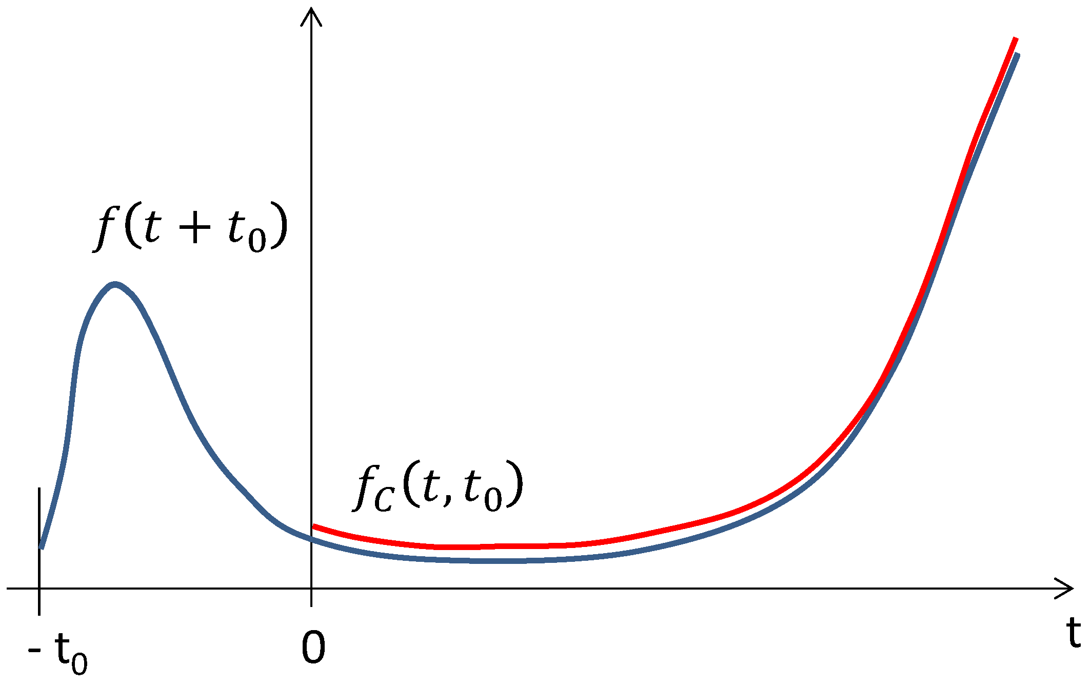
On the basis of the failure pdf model defined in Equation (22), we propose the model of the failure pdf of a used component. We define $t$ = 0 as the time of birth of the device and $t_{0i}$ the time of birth of the i-th component. Therefore, we define the conditional failure probability, given the fact that the component produced at time –$t_0$ has no failure at time t = 0, as:

$$f_C\left(t,t_0\right)=\frac{f\left(t+t_0\right)}{1-{{\displaystyle \int }}_0^{t_0}f\left(\tau \right)d\tau }=\frac{f\left(t+t_0\right)}{1-F\left(t_0\right)}; t\ge 0$$

(29)

Figure 2 shows the conditional failure pdf of a used component and how it is obtained from the failure pdf. The fact that the used component survived the infant mortality increases the reliability of the used component with respect to a new one.

The dismounting and remounting of a component in a new board may cause an additional stress, we propose to model this effect as an additional “infant mortality” $f_s$ using a gamma function.

$$f_s\left(t\right)=\frac{{\beta }_s{}^{{\alpha }_s}}{\mathsf{\Gamma }\left({\alpha }_s\right)} t^{{\alpha }_s-1}{e}^{-{\beta }_{s}t}$$

(30)

The pdf of the used component $f_R$ is, therefore:

$$f_R\left(t,t_0\right)=b_s{f}_s\left(t\right)+b_C{f}_C\left(t,t_0\right)$$

(31)

with the normalization condition:

$$1=b_s+b_C$$

(32)

If a component is new, that is $t_0=0$, there is no additional stress for dismounting and it results in:

$$f_R\left(t,0\right)=f_C\left(t,0\right)=f\left(t\right)$$

(33)

Combining previous equations with Equation (22) we obtain:

$$f_R\left(t,t_0\right)=b_s{f}_s\left(t\right)+b_C\left[a_{\lambda }\frac{f_{\lambda }\left(t+t_0\right)}{1-F_{\lambda }\left(t_0\right)}+a_{\mathsf{\Gamma }}\frac{f_{\mathsf{\Gamma }}\left(t+t_0\right)}{1-F_{\mathsf{\Gamma }}\left(t_0\right)}+a_G\frac{f_G\left(t+t_0\right)}{1-F_G\left(t_0\right)}\right]=b_s{f}_s\left(t\right)+b_C\left[\frac{f\left(t+t_0\right)}{1-F\left(t_0\right)}\right]$$

(34)

with cumulative function:

$$F_R\left(t,t_0\right)={{\displaystyle \int }}_0^t{f}_R\left(\tau ,t_0\right)\mathrm{d}\tau =b_s{F}_s\left(t\right)+b_C\left[\frac{F\left(t+t_0\right)-F\left(t_0\right)}{1-F\left(t_0\right)}\right]$$

(35)

The models of the pdf $f_R\left(t,t_0\right)$ and of the failure cumulative probability $F_R\left(t,t_0\right)$ will be applied in Section 6 to used components for different values of $t_0$, which is the life of the component before it is mounted on a new device.

5. Design for Reuse and Reliability

Electronic equipment consists of many components. The failure rate of the equipment composed of N components with independent failure rate is [20]:

$${\lambda }_E\left(t\right)={\displaystyle \sum }_{i=1}^N{\lambda }_i\left(t\right)$$

(36)

Therefore, the cumulative probability of failure of the equipment made of N components becomes, using Equations (7) and (36):

$$F_E\left(t\right)=1-{\mathrm{e}}^{-{{\displaystyle \int }}_0^t{\lambda }_E\left(\tau \right)d\tau }=1-{\mathrm{e}}^{-{{\displaystyle \int }}_0^t{{\displaystyle \sum }}_{i=1}^N{\lambda }_i\left(\tau \right)d\tau }=1-{{\displaystyle \prod }}_{i=1}^N{\mathrm{e}}^{-{{\displaystyle \int }}_0^t{\lambda }_i\left(\tau \right)d\tau }=1-{{\displaystyle \prod }}_{i=1}^N\left(1-F_i\left(t\right)\right)$$

(37)

In case some of the components are reused, Equation (37) becomes the following:

$$F_E\left(t;t_{0,i}\right)=1-{\displaystyle \prod }_{i=1}^N\left(1-F_{R,i}\left(t,t_{0,i}\right)\right)$$

(38)

When the failure probability is low, as in the test case reported in this work, in which the cumulative failure probability is less than 0.1%, Equation (38) can be approximated by:

$$F_E\left(t;t_{0,i}\right)\approx {\displaystyle \sum }_{i=1}^N{F}_{R,i}\left(t,t_{0,i}\right)$$

(39)

and

$$f_E\left(t;t_{0,i}\right)\approx {\displaystyle \sum }_{i=1}^N{f}_{R,i}\left(t,t_{0,i}\right)$$

(40)

The goal of a design for reliability is the maximization of the reliability of the equipment $R_E$ or the minimization of the cumulative probability of failure $F_E$. Maximum reliability means minimum failure rate $\lambda$, if we use a model of failure rate independent of time as in the IEC 62380 standard [15], Telcordia [16], or the exponential function in Equation (9). However, we must define the time interval in which we consider the reliability of the equipment if the failure rate depends on time, such as in the “bathtub curve” model or in the experimental measurements that we will show in the next section.

Usually the companies are interested in a reduced failure rate for the first 5–10 years and they are not interested in the behavior in the long term. Therefore, in this work we consider the minimization of the cumulative probability of failure of the device $F_E\left(t\right)$ in a fixed time t (for example, 5–10 years).

The goal of a design for reuse and reliability is the minimization of the cost of the equipment, where the cost takes into account the cost of the components, the social cost of waste management of the broken equipment that we substitute with the new one and the cost of repair of the new equipment in case of failure. The last term considers the reliability of the new equipment. Even in this case the total cost of the equipment should be referred to as the predefined amount of time in which we consider the reliability of the system (for example, 5–10 years). The total cost of the equipment can be defined in the following way:

$$C_E\left(t,t_0\right)={\displaystyle \sum }_{i=1}^N{C}_{R,i}\left(t_{0,i}\right)+{\displaystyle \sum }_{i=1}^N{C}_{D,i}+F_E\left(t;t_{0,i}\right)\left(C_S+{\displaystyle \sum }_{i=1}^N{C}_{R,i}\left(t_{0,i}\right)\right)$$

(41)

where the first term is the cost of the new device, the second term is the cost of disposal of the device that we replace with the new one and the third term is the cost of the repair of the new device in case of failure. The device is composed of N components, and:

• $C_{R,i}(t_{0,i})$ is the cost of the single component that can be new or used; if used its cost on the market depends on its reliability that depends on its previous life and its age;
• $C_{D,i}(t_{0,i})$ is the cost of collection, dismounting and disposal of the single component. If the component is for reuse the cost of disposal is zero;
• $F_E\left(t;t_{0,i}\right)$ is the probability of failure of the equipment defined in Equation (38) that depends on time and the age of the used components;
• $C_S$ is the cost of the collection of the equipment for repair.

The cost of a new component is:

$$C_{R,i}\left(t_{0,i}=0\right)$$

(42)

If for simplicity, we neglect $C_S$ and $C_D$ we obtain:

$$C_E\left(t,t_0\right)=\left[1+F_E\left(t;t_{0,i}\right)\right]{\displaystyle \sum }_{i=1}^N{C}_{R,i}\left(t_{0,i}\right)$$

(43)

Equations (38)–(43) define the model that can be used for the design for reuse and reliability of electronic equipment. The first phase of data collection for the development of the reliability model and the estimation of the parameters of the failure probability model are fundamental for the accuracy of the model itself. The defined framework has been used in the analysis and design optimization of a real test case is shown in the next section.

6. Results of a Real Test Application

The design methodology has been applied to the boards of the control system of elevators of the Vega S.r.l. company. Two commercial boards have been studied: the control board of the display of the elevator, that we will call TFT, and a control board of the elevator, named Control. The components of the electronic equipment of this specific application do not suffer from the problem of obsolescence, as in other applications like smartphones. Therefore, the reuse of the single component is possible without problems and with economic advantages even without considering the disposal costs.

The historical data of the three types of boards produced and sold in the last eight years have been recorded and stored in a database: the date of production, date of failure, type of failure, component/components responsible for the failure and type of repair.

Even if eight years is a long period of time, the estimation of the failure rate is not accurate for the aging zone. The reliability has been therefore considered for 5- or 10-year periods but not longer. On the other hand, longer time windows are not relevant from a commercial point of view.

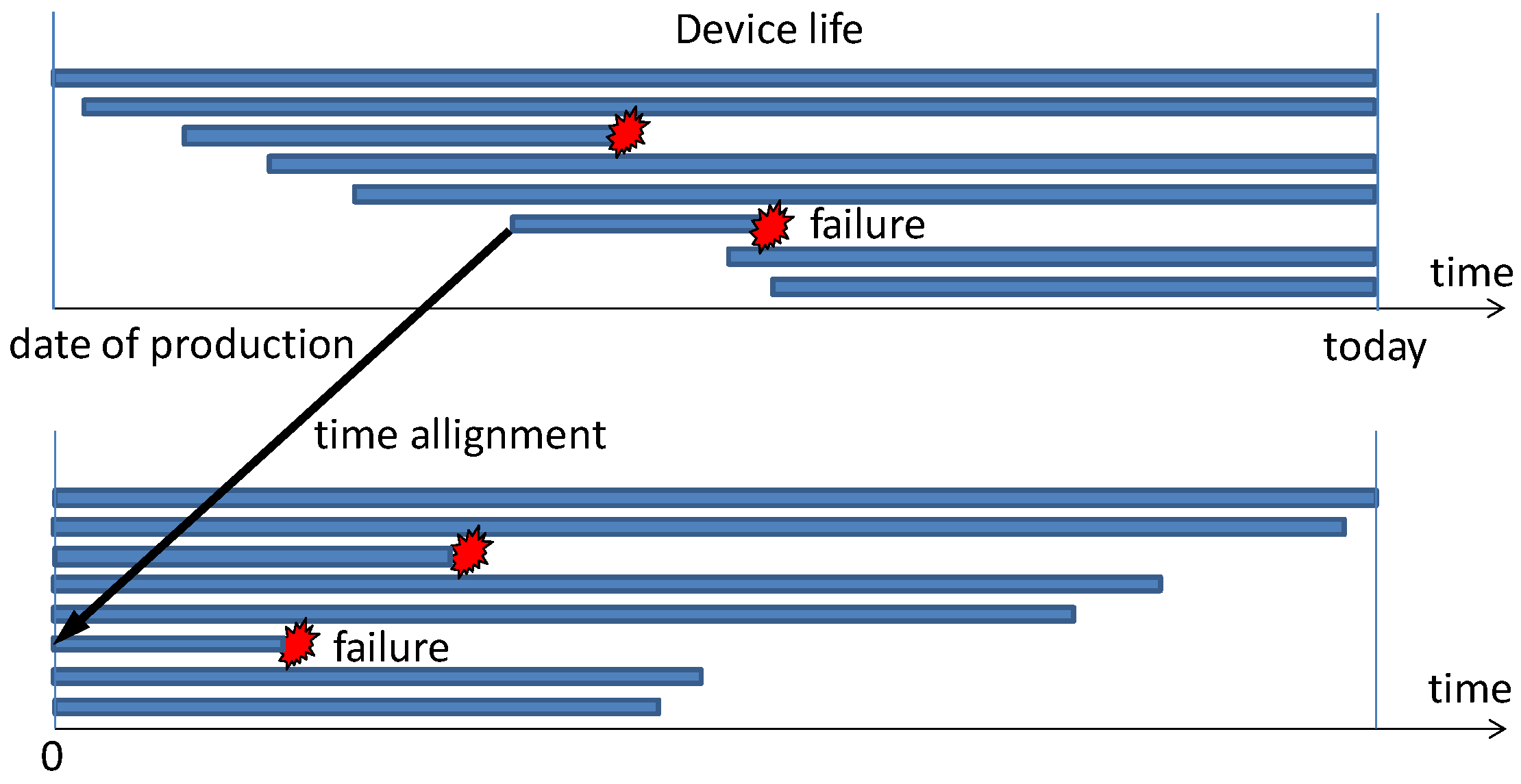
The two types of boards were introduced eight years ago and they are currently under production. Therefore, they have a different date of production and installation, as shown at the top of Figure 3. In order to compare the data, a time alignment at the instant of production was performed and shown at the bottom of Figure 3.

Figure 4a shows the number of failures for each month over time. Figure 4b shows the sample size over time and it is evident that the number of monitored products changes over time: few of them have eight years of life. Figure 4c represents the failure rate over time obtained by dividing the number of failures over time (Figure 4a) by the number of products over time (Figure 4b).

The data was collected for each component of the two boards and the reliability parameter estimation was performed for each component as described in Section 3:

• IEC 62380 standard: the mission profile was defined for each component and the failure rate $\lambda$ calculated using the EIC 62380 model. As an example, we report some of the parameters we used for the microcontroller on the basis of its use: average ambient temperature equal to 18 °C, the temperature of the board close to the component equal to 21 °C, average temperature excursion of the board equal to 5 °C and working phase always on.
• Telcordia standard: failure rate $\lambda$ was calculated using the Telcordia model.
• Experimental measurements: the failure rate was evaluated from the historical failure data, after time alignment and normalization as described in Figure 3 and Figure 4.
• Model: our model presented in Equation (22) was used. The parameters for each component were determined to minimize the error between the experimental cumulative probability of failure and the model.

The model was compared with the historical data in Figure 5, Figure 6, Figure 7, Figure 8 and Figure 9 for some of the components of the two products. Figure 5 shows the pdf of the microcontrollers for the first 10 years of life: experimental data, model and the single components of the model consisting of gamma function for infant mortality, the exponential function for the random failure and the normal function for the aging effect. The data were collected each month. 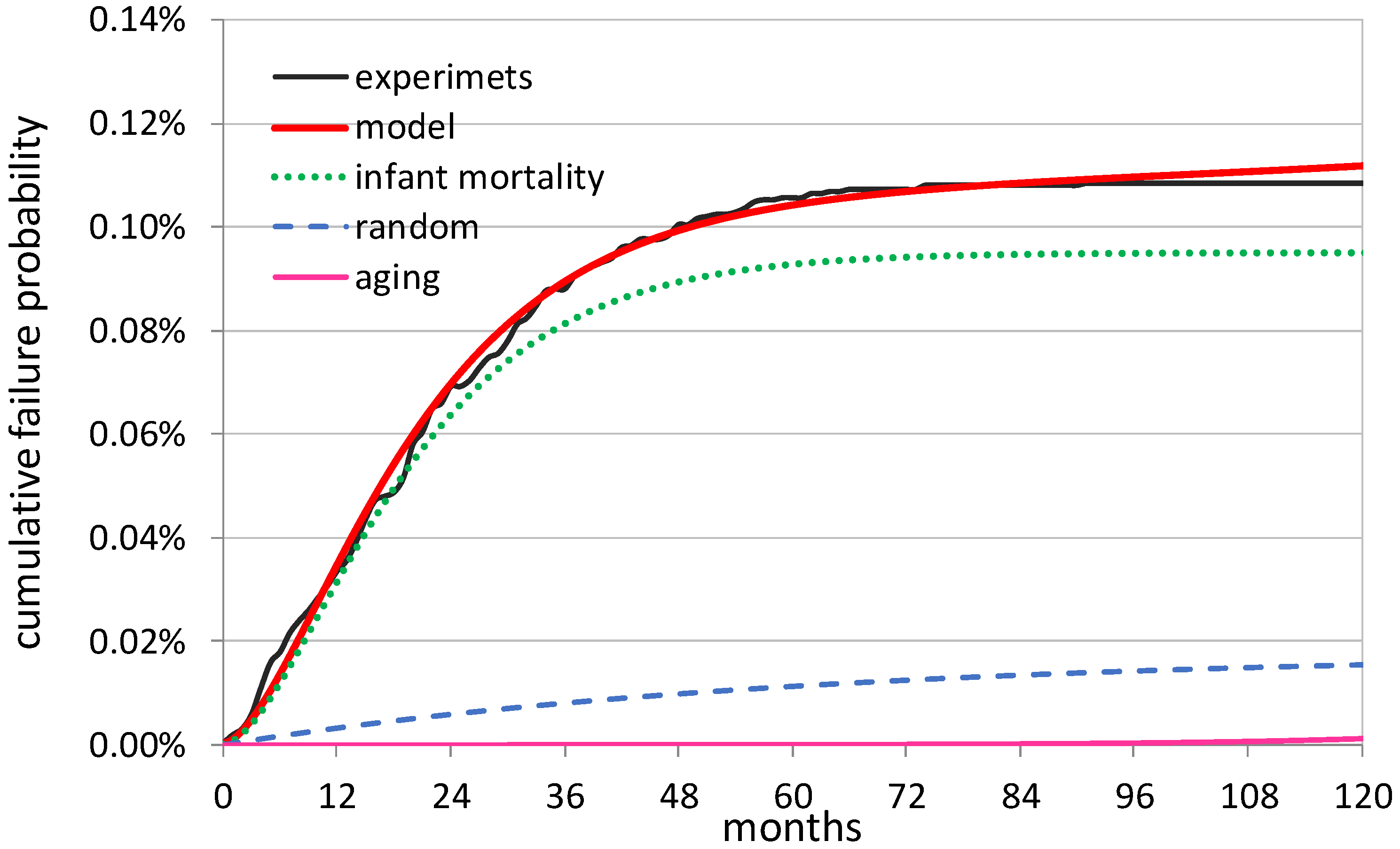Figure 6 shows the cumulative failure probability function of the microcontrollers for the first 10 years of life: experimental data, model and single components of the model. The agreement between historical and model data is good. The aging effect is not relevant for the first 10 years and the maximum failure after 10 years is low, about 0.1%.

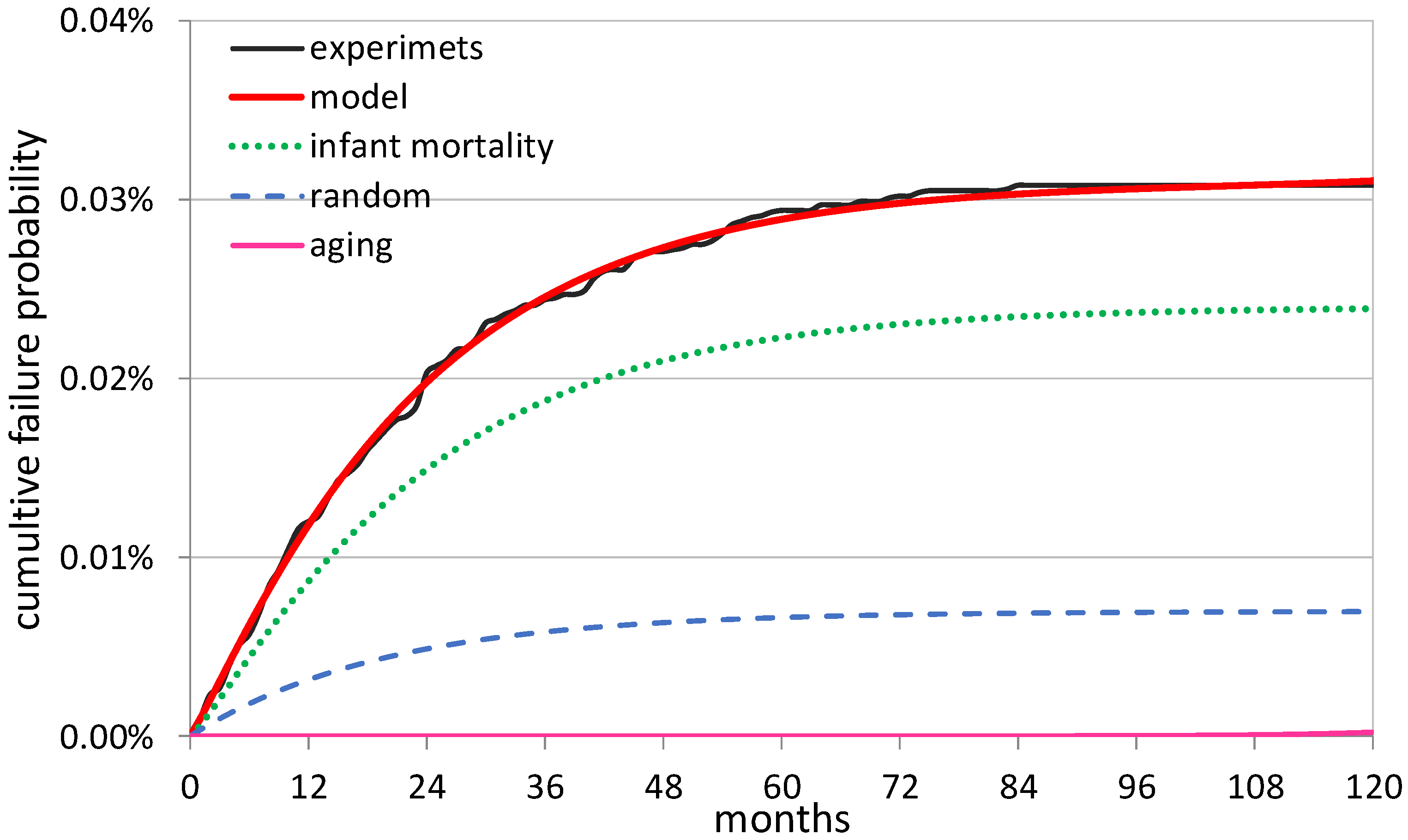
Similarly, Figure 7 and Figure 8 show the pdf and cumulative failure probability function, respectively, of the Integrated Circuits for the first 10 years of life.

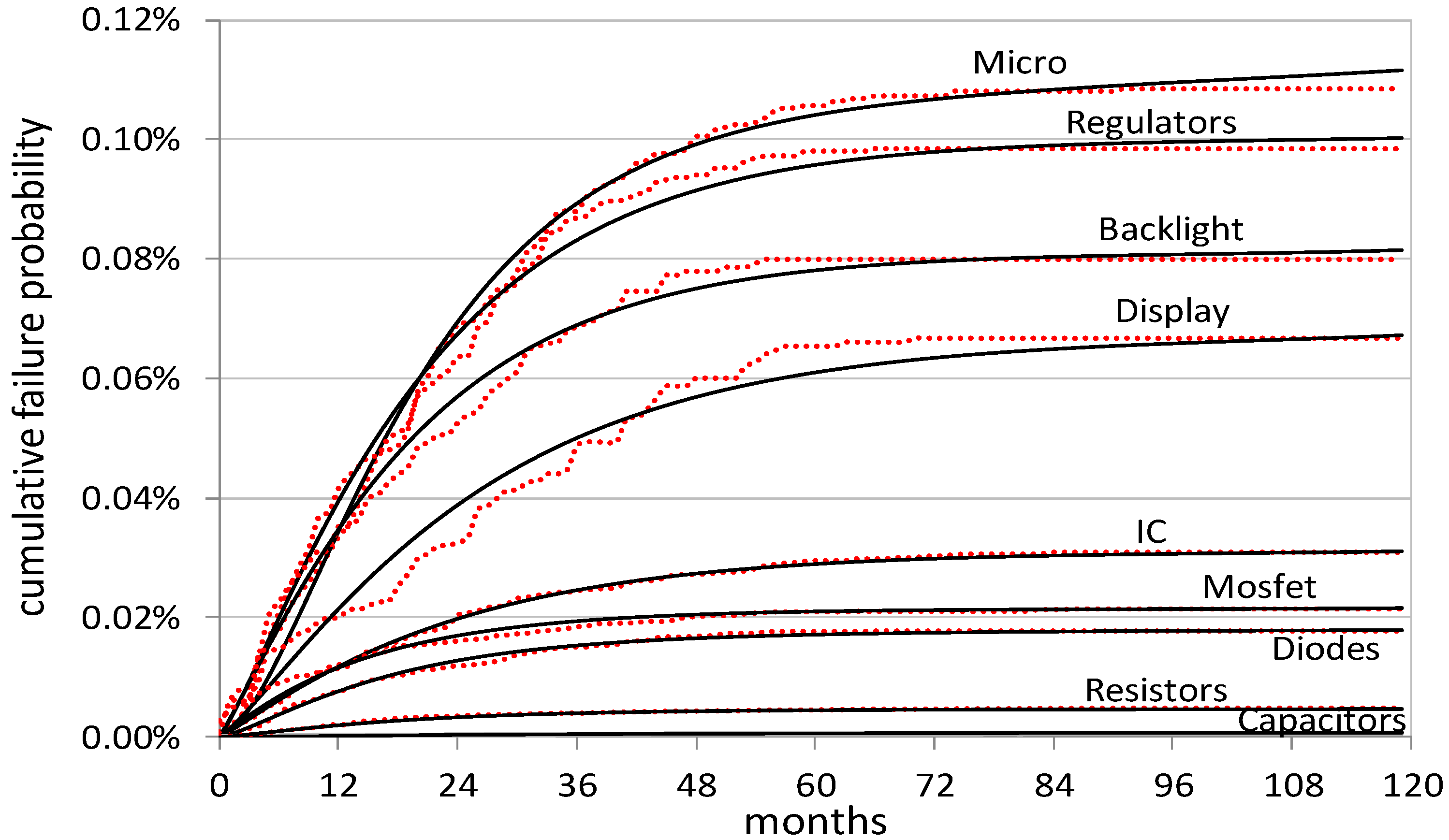
Model (in continuous lines) and historical data (dots) of the cumulative failure probability function of the main components are reported in Figure 9. It can be seen that for all the components the error is very low.

Table 1. Table of coefficients of the failure model.

Component	GAMMA			EXP		NORMAL
	α	β (months−1)	aΓ	λ (months−1)	aλ	μ (months)	σ (months)
Microprocessor	1.90	11	9.5 × 10−4	60	1.8 × 10−4	500	90
IC	1.20	20	2.4 × 10−4	20	7.0 × 10−5	350	50
Regulator	1.40	16	8.0 × 10−4	15	2.0 × 10−4	390	60
Backlight	1.55	15	5.6 × 10−4	11	2.5 × 10−4	360	55
Display	1.40	18	4.7 × 10−4	30	2.0 × 10−4	380	60
Diode	1.50	11	1.3 × 10−4	30	5.0 × 10−5	300	35
Mosfet	1.20	15	1.6 × 10−4	8	5.5 × 10−5	330	45
Capacitor	1.20	20	3.5 × 10−6	50	3.5 × 10−6	390	52
Resistor	1.40	13	3.3 × 10−5	22	1.4 × 10−5	390	55

reports the coefficients of the model for each component, as obtained by the fit with the cumulative failure probability.

A comparison between the results of the four methodologies consisting of IEC, Telcordia, our model and historical data was performed.

Table 2. Failure rate of the single components expressed in FIT (FIT = 1/${10}^9$ h) for the four methodologies: Telcordia, IEC experimental data and our model.

Component	$\mathit{\lambda }$ (FIT)
	Measure (0–7) Y	Measure (0–2) Y	Model (0–7) Y	Model (0–2) Y	Telcordia	IEC
Microprocessor	16.4	38.2	20.3	41.2	22	65
Flash Memory			15	35	20	45
SDcard	15	18	30	65	60	353
Regulator	16.3	35.4	19	41.3	14	44
IC	16.9	35.7	22.4	43.1	18	398
Display	12.8	24.7	16.8	27.5	31	380
Mosfet	3.2	9.2	3.7	9.7	1.7	42
Diode	3.8	8.9	3.1	7.1	1.7	42
Capacitor	0.1	0.2	0.3	0.4	0.2	0.2
Resistor	0.8	2	1	2.1	0.51	0.03
Microprocessor	16.4	38.2	20.3	41.2	22	65

reports, for the four methodologies, the failure rate $\lambda$ expressed as failures in time (FIT) rate, which is the number of failures that can be expected in one billion (${10}^9$ h) device-hours of operation. Telcordia and IEC give a constant value of the failure rate, whereas the failure rate depends on time for the experimental data and our model. To compare the results, the average value over the first three years (where the infant mortality is relevant) or the first eight years was calculated.

The results confirm a good agreement between historical data and our model. The error is relevant between Telcordia/IEC and data, due to the fact that those models take into account the information on the datasheet and mission profile and not the experimental data. In fact, Telcordia and IEC are used, in general, when experimental data are not available. Furthermore, the infant mortality gives a relevant contribution to the failure rate: for example, 38.2 FIT is the failure rate in the first three years and 16.4 in the first eight years. This aspect makes the reuse of components in the fabrication of the board convenient since the used components survived the infant mortality.

The failure rate of the single components has been used to estimate the failure rate of the equipment under production using Equation (32) for equipment composed of N components with independent failure rate.

Figure 10 shows the contribution to the failure rate of the TFT board of different types of components. The data are derived from historical failure data, considering the component that was the reason for the fault. From the historical data we verified that a joint fault of more than one component is negligible. Display, diodes and IC are responsible for about 60% of the faults.

Similarly, Figure 11 shows the contribution to the failure rate of the Control board of the different types of components. The SD card, Amplifier and DAC were responsible for about 70% of the faults.

TFT and Control are boards under production. We redesigned the Control board on the basis of the analysis of the failure data. The Control_new is the redesign of the Control board in order to reduce the failure rate and on the basis of improvement of the product. The main change in the Control_new board with respect to the previous version was made with the aim of reducing the failure rate and it consisted of the addition of a flash memory in conjunction with the existing SD card, as the faults related to the SD card were related to the loss of data due to frequent access. The flash memory with a higher data retention period limits the access to the SD card only to reprogram the memory. Another change consists of the substitution of the regulator with a new one able to work with higher voltages and with additional protection devices. These changes allow an expected reduction in the failure rate, as reported in

Table 3. Failure rate of four boards expressed in FIT (FIT = 1/${10}^9$ h) for the four methodologies: Telcordia, IEC experimental data and our model.

Board	$\mathit{\lambda }$ (FIT)
	Measure (0–7) Y	Measure (0–2) Y	Model (0–7) Y	Model (0–2) Y	Telcordia	IEC
TFT	248	738	467	870	364	3733
Control	585	720	364	630	292	2340
Control_new			321	549	259	1448

.

Figure 11 shows the contribution to the failure rate of the Control_new board of the different types of components. The results are derived from the failure model of the components and the use of Equations (36) and (37) to estimate the failures of the board.

Table 3 reports the failure rate of the three boards expressed in FIT for the four methodologies: Telcordia, IEC, experimental data and our model. The count of failures of the boards was used for the experimental data, while Equations (36) and (37) were used for the models.

Our model and experimental data are in acceptable accordance. Since Telcordia and IEC give a constant value of the failure rate, they are not able to take into account the infant mortality. This is evident from the fact that the failure rate is higher in the first three years with respect to the first eight years. Furthermore, the IEC model highly overestimates the failure rate.

The changes in the control board allow an expected reduction of the failure rate, as reported in Table 3. This reduction is mainly due to the use of the flash memory, as can be seen by comparing Figure 11 and Figure 12.

Finally, the proposed model of cumulative failure probability of used components has been applied to estimate the reliability of the boards manufactured with one-year-old used components. As already shown, the infant mortality of the components is relevant, and the cost of some new components is high. As in the pre-burning methodology, the reuse of components allows for the reduction of infant mortality.

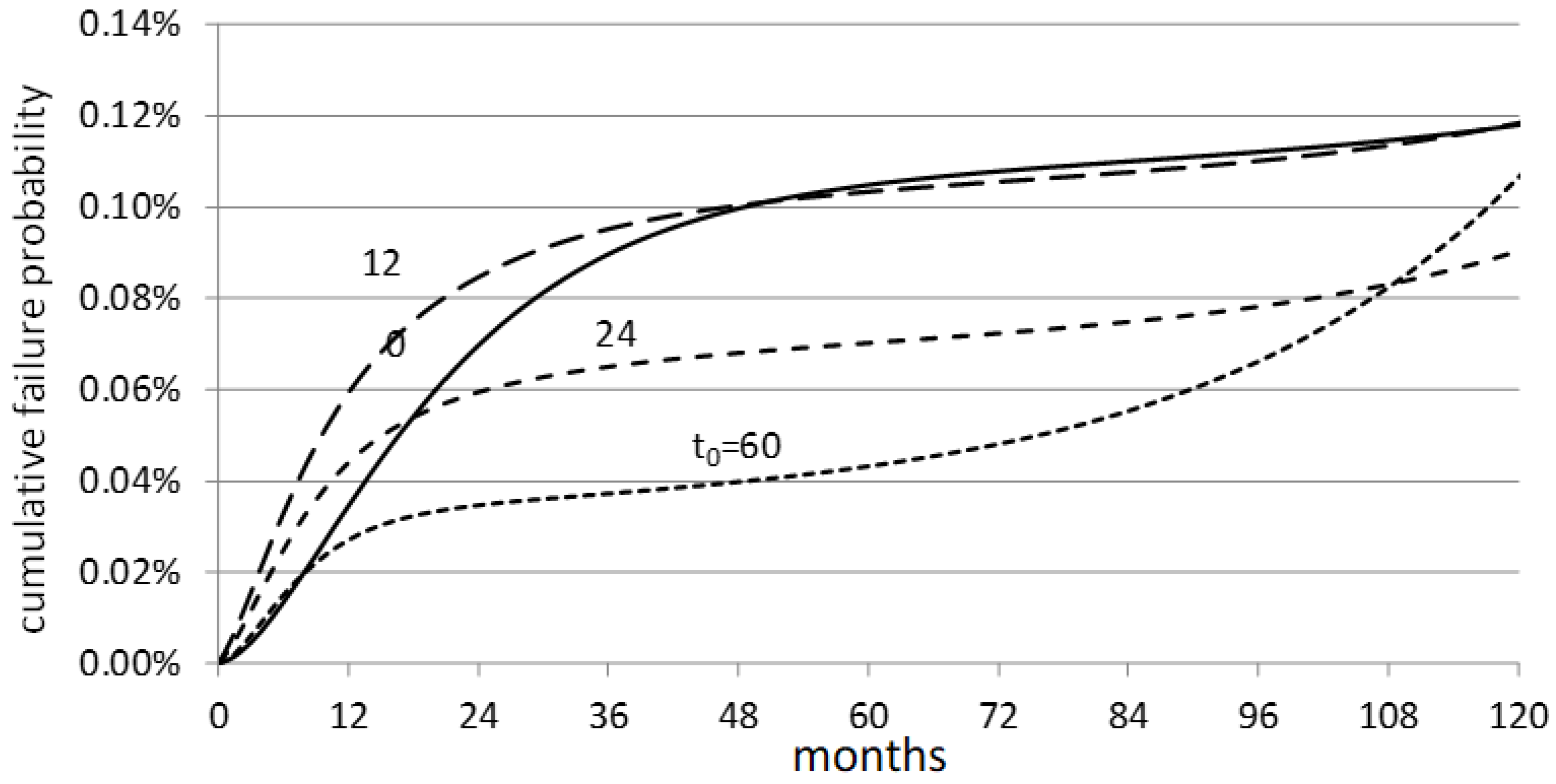
As an example, Figure 13 reports the pdf $f_R\left(t,t_0\right)$ of a used microcontroller component as a function of time for different values of $t_0$, that is the life of the component before it is mounted on a new device. Similarly, Figure 14 reports the cumulative failure probability $F_R\left(t,t_0\right)$.

The case of a new component corresponds to $t_0$ = 0. The additional “infant mortality” $f_s$ due to the stress remounting of the component in the new board has been considered. Figure 13 and Figure 14 show that the reuse of a component reduces infant mortality, partially reintroduced by the remounting stress, but it anticipates its aging.

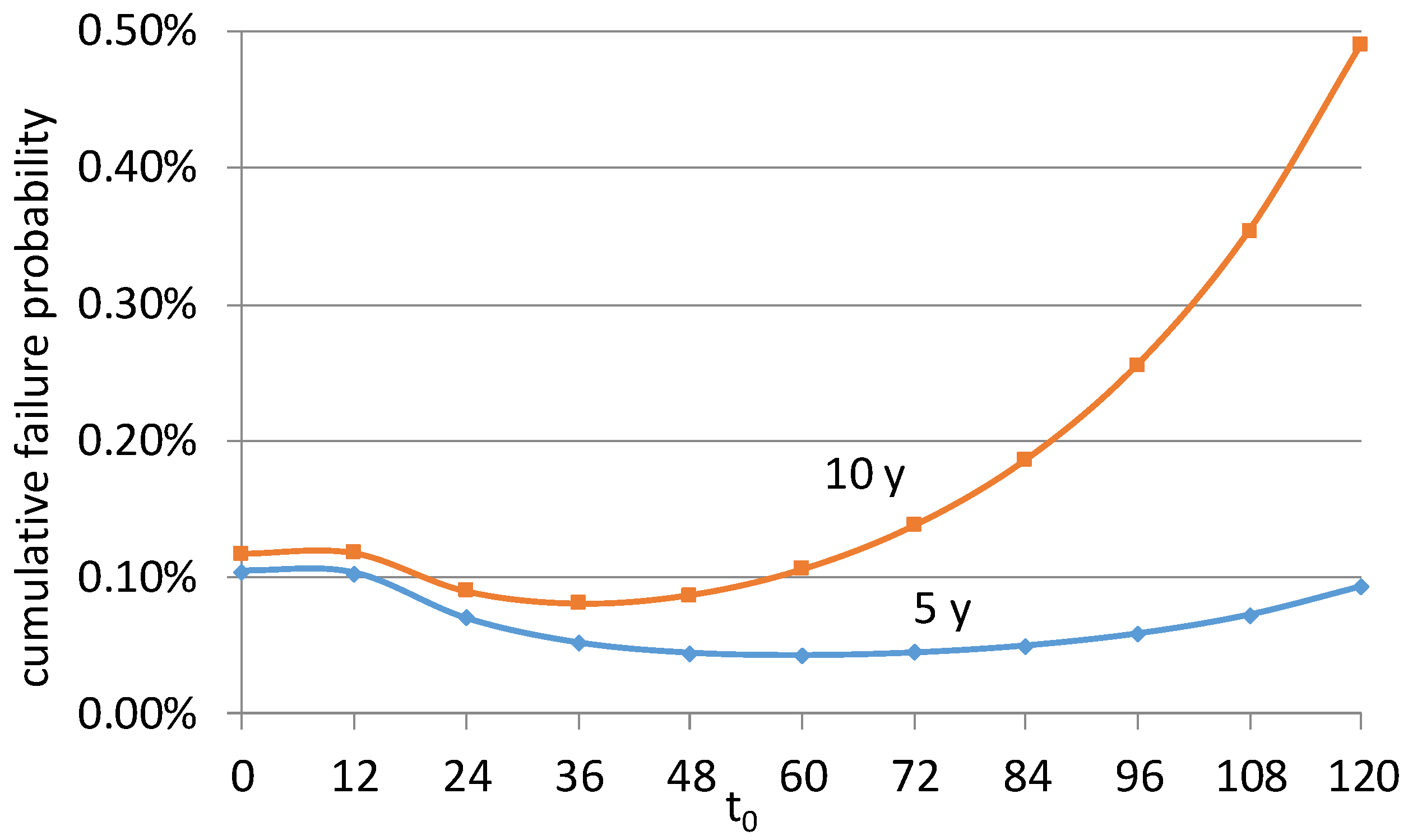
Conversely, Figure 15 shows the cumulative failure probability of the used microcontroller after five or ten years as a function of its previous life. Young used microcontrollers are more reliable than new ones. When $t_0$ is too high (old used microcontrollers), the reliability is worse.

The failure probability has been estimated after five and ten years for the three boards.

Table 4. Estimated cumulative failure probability using new components or used components in the three test boards.

Board	Failure 5 Y		Failure 10 Y		Failure 15 Y
	New	Reused	New	Reused	New	Reused
TFT	2.10%	0.93%	2.50%	1.33%	3.45%	4.46%
Control	1.43%	0.90%	1.62%	1.11%	2.24%	3.20%
Control_new	1.20%	0.66%	1.40%	0.88%	2.02%	2.97%

reports the estimated cumulative failure probability using new components or one-year-old used components. The advantages of reusing components are evident for the first ten years.

An additional consideration must be drawn with regards to the cost of disposal of used boards and the cost of buying a new component for the new board. We have shown that the reuse of components in many cases gives an advantage in terms of the reliability of the equipment. If the cost of the new component is high, an economic advantage is evident, too.

Table 5. Failure rate and cost of some components of the Control_new board.

Component	IEC $\mathit{\lambda }$ (FIT)	Cost
Microcontroller	65	4.30 €
Flash mem	45	3.60 €
IC (transceiver)	23	2.50 €
IC (digital reostat)	14	0.75 €
Switching Regulator	3.4	0.57 €

reports some relevant components in terms of the cost of the Control_new board, whose reuse is interesting both in terms of reliability and economic impact.

7. Conclusions

The reliability analysis, modeling and optimization of electronic equipment have been widely studied for a long time. In recent years, the problem of the reduction of WEEE has been faced, in connection with the concept of circular and green economy. The design of electronic systems for EoL considers the possibility for repair, reuse and recycling, in order to reduce waste.

This work proposes a new accurate model of failure probability density, that includes the failure probability of used components in new equipment. The model has been tested, in conjunction with the standard IEC and Telcordia in real industrial production. Eight years of historical faults have been analyzed to derive the fault models of the components. The model and analysis were used for the study of two pieces of equipment and the results were used to redesign one board.

In the near future, we can have the real verification of the reliability improvement of the new control system designed. Another key point, that we will verify, is the experimental evaluation of the effect of the dismounting stress on the components. Nevertheless, the positive message that we want to transmit is that a good redesign of electronic equipment and the reuse of components could make an improvement to the reliability of the equipment, in addition to waste reduction.

The mathematical framework we propose can be used in different applications. The framework has been much more accurate than the commonly used standards, such as IEC 62380 and Telcordia. The acquisition of field data is fundamental for ensuring the accuracy of the prediction.

Nevertheless, the verification of the relevance of the infant mortality with respect to the other causes of faults can be quickly verified, since it happens in the first years of the life of the product.

Other aspects, connected to the design for reuse and reliability, are the modular design [21] and traceability of the electronic components. The use of RFId for traceability is applied in a wide variety of applications: food [22,23], organic waste [24], integrated circuits [25] and WEEE waste [12,13,26,27,28].

The partitioning of boards into modules could allow for the speeding up of the disassembly process, to reduce the amount of WEEE and to reduce the fault probability of the complete system by replacing the single module.

The accurate modeling of the reliability of each component, new and used, is fundamental for component reuse and modular design. Conversely, electronic component traceability is fundamental for the estimation of the residual life of the used components and for the creation of a market of used devices. A real-time database based on RFId can be used to track the history of a board or component, and this information can be used to make better end-of-life decisions.