Article

Energy–Economy Coupled Simulation Approach and Simulator Based on Invididual-Based Model

School of Electric Power Engineering, South China University of Technology, Guangzhou 510641, China
*
Author to whom correspondence should be addressed.
Current address: 381 Wushan Road, Tianhe District, Guangzhou, China.
Energies 2020, 13(11), 2771; https://doi.org/10.3390/en13112771
Submission received: 2 April 2020 / Revised: 18 May 2020 / Accepted: 25 May 2020 / Published: 1 June 2020

Abstract

:
An integrated energy system, referred to specifically as a heterogeneous energy system that combines cooling, heating, power, etc., is a dynamic system containing continuous as well as discrete behaviors on both technical and economic levels. Currently, the comprehensive utilization of multiple forms of energy and the implementation of the energy market have made the simulation of such a system very complicated, which is reflected in two aspects. First, the simulation model becomes complex and varied. Second, the time-varying characteristics of the models are quite diverse. Therefore, a standard and normative modeling and simulation method is urgently needed. This work aims to obtain a compatible modeling and simulation method for the energy economy coupling system. The individual-based model is widely used to describe organisms in an ecology system that are similar to the energy–economy coupled system. Inspired by this, a general simulation approach based on the individual-based model is proposed in this paper to overcome these existing problems. The standard formal expression model is built, then its structure and elements explained in detail, and multi-scale time simulation supported to model and simulate an integrated energy system that is coupled with markets. In addition, a simulator is designed and implemented based on multi-agent framework and model-view-controller architecture. Finally, a simulation case of a conceived scenario was designed and executed, and the results analysis proved the validity and versatility of the proposed approach. The proposed method has the advantages of model standardization, multi-scale time compatibility, distributed simulation capability, and privacy protection. These advantages support and strengthen each other. Through these studies, a systematic approach was formed that could improve the standardization of modeling and simulation in the energy–economy research area.

Graphical Abstract

1. Introduction

Owing to the graded and complementary use of energy, an integrated energy system (IES) has considerable advantages as it enables more efficient use of energy and is advocated in many countries and regions. At the same time, market-based competitive transactions are being implemented with greater coverage in several energy sectors, which cause the study of physical energy systems and financial market transactions to be often intertwined [1]. The research objects of this topic include not only energy devices with different physical properties and members with economic decision-making properties, but also bidirectional influences between the two. Therefore, such a system is also called the energy–economy coupled system (EECS). Among methods used to research the EECS, modeling and simulation (M&S) plays a very important role in energy planning programming, policy making, and dynamic analysis. The core technology for an EECS simulation exists in two aspects: system level specification and model specification formalism. The former refers to the operating principle of the simulation system, while the latter declares the structure and elements of the model.
Currently, in the fields of energy and economy research, both have their own simulation methods and scope, according to the characteristics of the study object concerned. For example, in power system research, dynamic simulations such as electromagnetic and electromechanical transient simulation programs based on different numerical calculation methods are used. Regarding a multi-energy system, several energy modeling and planning systems were built based on GAMS (the General Algebraic Modeling System), such as TIMES [2] and its original version MARKAL [3]. For an overview, the reader is referred to [4], in which a detailed introduction to 68 energy tools is given. Similarly, 24 different energy optimizers and simulators are summarized in [5], adopting multiple evaluation criteria, such as time and spatial resolution, an analytical approach, and a programming environment. Economic systems also feature a variety of simulation methods, such as agent-based simulation [6,7] and system dynamics simulation [8]. Among numerous modeling and simulation approaches, agent-based simulation is popular for its distributed ideology, which is suited to a multi-component and non-centralized coordination system. In multiple research areas, including the brain, immune system, ecosystems, societies, and financial markets, an agent-based approach has been widely applied [9]. For example, ASPEN (an agent-based simulation model of the U.S. economy) developed by the Sandia National Laboratories has long played an important role in energy policy research [10]. Individuals in the ASPEN model represent real-life economic decision-makers, including households, banks, government, the Federal Reserve, and firms. In the field of computational economics, AMES is used to simulate spot electricity market transactions based on node price [11].
Just in terms of quantity, there is no shortage of energy or economy simulation tools, but to study dynamic interactions between different sub-systems their integration in one simulation environment is necessary [12]. A coupled simulation that combines a bottom-up/top-down approach shows its potential in energy–economy–environment (3E) prospective modeling, which is worthy of attention [13]. Current research attempts to achieve coupled simulation by connecting different simulation tools [14]. For instance, in [15], a soft-linking of a power systems model to an energy system model is presented. Both models exist as themselves in a simulation system, i.e., PLEXOS [16] and TIMES [17]. Furthermore, in [18], an architecture that tries to encompass any tool that aims to model the energy sector is proposed. Distributed simulation offers strong computing power and less computing time based on multi-thread simulation technology. These features are the reasons distributed simulation is widely used in complex system simulation. It is difficult to implement parallel simulation through the joint simulation of software connections due to limitations of interface authority. In addition, the data format or application interface of each system is different, and each application must develop special data interface conversion programs for other applications to realize information sharing. In the absence of a common data interface/model, the number of data converter programs required by N applications is C N 2 = N · ( N 1 ) 2 , which requires significant human effort to implement mappings.
Regarding a model specification formalism, generic and scalable models have also received considerable attention. Modelica [12] is an open, object-oriented, equations-based language that can only model complex physical systems across different fields. PRIMES is a 3E model developed by E3M-Lab in the institute of Communication and Computer Systems of the National Technical university of Athens [19], and its objective is to simulate energy systems and markets across Europe. The model in PRIMES provides detailed descriptions, including of energy production, emissions, and market, but it still does not involve more elaborate operations models, such as transient models. The Common Information Model (CIM), which is currently modeled as a UML, allows application software to exchange information about power systems [20] and energy market data [21]. It has been widely used in the field of power system modeling but not used in a general energy–economy coupled system. There are also optional agent development frameworks that can be adopted to code the simulation, but the programmer still must define the non-standard and user-defined model of the agents by writing code in a programming language. Thus, a unified modeling and simulation approach that is easily implemented is needed. Odell and Giorgini [22] summarized the existing meta-models of multi-agent systems from the perspective of software engineering, which attempts to propose a unified multi-agent model.
The simulation of EECS has four characteristics. First, almost all existing components in a system may change their intrinsic properties over time, such as the technical arguments, evolving behavior, and acquired data. Second, as a broad cross-disciplinary approach capable of capturing system-wide interdependencies [23], such a simulation system contains a large number of individuals and requires a broader modeling scope, not only with respect to energy devices, but also active market players. Third, interactions between individuals exist universally [24]. Fourth, the time-varying characteristics of individuals vary greatly, so that multiple simulation timescales coexist, from long-term investments and de-carbonization strategies to short-term operational and even transient process aspects of systems.
Regarding the aforementioned characteristics, requirements for simulation platforms of EECS are introduced. First, the platform should adopt a general and extensible model or interface that can be compatible with different types of individuals to facilitate the easy design and development of simulations. Second, the platform should enable parallel computing to decompose computing tasks. Because the simulation system contains a large number of individuals whose decision-making may be very complicated, and some small-step simulations have high calculation frequency, the amount of calculations is very large, so that parallel computing and distributed simulation are needed. Third, multiple-timescale simulation deserves strong support for different frequency individual characteristics, considering long-term perspectives as well as short-term operational details. Fourth, the platform requires dynamic simulation ability for complex adaptive systems.
The individual-based model (IBM) is widely applied in ecology [25]. The authors of [26] proposed a standard protocol called ODD (Overview, Design, and Details) to describe simulation models in the field of ecology. When ODD was proposed, it was intended to solve the problem of irregular complex model descriptions of ecology research papers in the case of limited space in academic journals. The protocol consists of three components: the overview, design concepts, and details. In the overview, the purpose of simulation, simulation variables, simulation scale, simulation step size, simulation calculation order, and other simulation information are included in detail. Design concepts contain a number of concepts. Details contain the simulation initialization configuration data, input data for the external environment, and the calculation subprocesses. The ODD protocol is a good idea that has been applied in many subsequent studies, and has been improved in a later updated version [27]. Energy–economy coupled systems comprise a complex system similar to an ecosystem, and the ODD protocol can also be used to describe simulation models of energy–economy systems. However, to adopt this protocol as a computable data model, many improvements must still be made, because it is not designed as a canonical computing model for the simulation of EECS, but rather a model for document description. In [28], attempts are made to apply the IBM in system dynamic analysis and the result shows that IBM can work well in IESs. At the same time, the IBM has superior characteristics, e.g., it is distributed and privacy-protected. The cross-disciplinary trend makes model compatibility necessary and possible, mainly through general software and standard protocols. In such a context, building a simulation platform suitable for the IBM must also be considered.
In summary, the IBM has the following characteristics: First, it describes a single entity, not the entire simulation system. This feature is in line with the bottom-up modeling idea, and can realistically describe the model details, resulting in the “emergent” behavior of the system. Second, the IBM is standardized in that it has a fixed form that applies to a wide variety of individual descriptions. Third, it is distributed compared to the centralized model. The IBM is expected to be applied more in the current climate of distributed research. Fourth, the IBM protects privacy. In the EECS, there are different interest subjects that put forward the requirement of information protection. The data contained in the IBM are readable only to subjects who have access to it, helping to protect individual privacy. Therefore, compared with existing models and tools, the proposed approach is more versatile for the cross-disciplinary EECS and has better compatibility with multiple models with significantly different characteristics. Moreover, the distributed idea makes it easier to decompose complex systems into multiple sub-parts, which interact with each other through communication. The decoupled IBM is used to realize the coupling simulation, which can not only adapt to the privacy protection needs of the energy market research but also study the overall performance of the whole system. A detailed technology characteristics comparison between the popular M&S methods and the proposed method is shown in Table 1. By comparison, we can see that the PRIMES is excellent among multiple existing methods. However, compared with the proposed method, it still lacks standardized model form, more compatible multi-scale time simulation, and adaptive distributed simulation ability. In Appendix A, the SWOT analysis matrix of the proposed method is presented (see Table A1).
For the reasons given above, in this paper, an attempt is made to address the two key issues in simulation and modeling aspects, considering that the IBM has the characteristics of being distributed, standardized, generalized, and to offer privacy protection. The main contributions of this paper are the following. (1) A review of the current state of simulation in the energy–economy field, including methods, tools, and shortcomings. (2) It improves the standardization with a proposed superstructure specification; that is, the modified IBM, consisting of a multi-tuple, which is defined and proved to be applicable to energy–economy coupled systems. In addition, an abstract interface is designed for a customized model solver. (3) Another forward-looking aspect of this study is to propose a coupled system simulation method that can be compatible with different simulation step sizes. (4) A programmable implementation scheme is provided. (5) A use case is designed to illustrate how the IBM works when applied in energy scenarios. The remainder of this paper is organized as follows. IBM and its general structure are explained, in particular, a full description of the elements of IBM, in Section 2. In Section 3, the simulation approach suitable for the IBM is presented. In Section 4, an implementation of simulation platform is described. Simulation results from runs of the proposed model and method, as well as its related analysis, are also presented in Section 5. Finally, conclusions and future prospects are given in Section 6.

2. IBM for EECS Simulation

An IBM models not only energy physical systems, but also energy economic, social, and cyber systems that affect the physical system. Therefore, the individual may be a physical device, financial market, data interface, or even a test rag. Almost all individuals can be modeled using an IBM. In addition, multiple relationships exist among individuals, resulting in individuals in the IBM of an EECS at different scales. For example, a thermal power plant individual usually contains more than one generator unit individual. Furthermore, each generator unit individual contains sub-units, such as exciter, steam turbine, and heat pump individuals. Figure 1 shows a common energy–economy coupled scenario consisting of multiple individuals of different types and sizes. Using mathematical set theory, the IBM can be formulated as Equations (1) and (2) in the form of five-tuples. The model describes individuals in detail without redundant data:
= I , M , S , F , O
M = ( ID , T , A , C , W ) ,
where denotes any target individual or component; I and O denote individual’s inputs and outputs; and M denotes static model of the individual that presents inherent attributes, including a globally unique identifier (ID), type (T), argument set ( A ), connectors ( C ), and subset ( W ). S is an individual’s state set and F denotes the function set that defines an individual’s dynamic behavior. All elements are described in detail below.

2.1. Input and Output

I and O are coupling artifacts among multiple individuals. Specifically, I means their external input events that describe environmental conditions and O means that an individual can also post external output events. I and O in Equation (3) denote an individual with m inputs and n outputs, respectively:
I = { x 1 , x 2 , , x m } O = { y 1 , y 2 , , y n } .
During the simulation, an individual will provide updated values for the output variables, which serve as input variables for other individuals. The contents of input and output are multiple flows, including information flow, cash flow, and energy flow. Information flow represents information exchanged between individuals, such as price information that an exchange publishes to market participants. Cash flow represents the financial income or expenditure generated by the activities of individuals. Energy flow represents the energy production and consumption at the physical mechanism level, and it obeys the fundamental laws of physics, such as the conservation of energy and Kirchhoff’s laws.
During the actual modeling process, one can also do some special processing on individual input and output. For example, a source can be regarded as an individual with no input and n outputs. A sink can be regarded as an individual with m inputs and no output. A converted individual (such as a transformer) can be seen as an individual with m input and n outputs [41].

2.2. Static Model

The static model M describes the general and characteristic parameters of an individual with five elements, namely ID , T , A , C , and W , as shown in Equation (2). ID (identification) is a means to identify an individual and it should be immutable and globally unique. It can be expressed by a name or sequence number so that any one individual will be marked with I D . T (type) denotes the classification of individuals corresponding to the conception Class in object-oriented programming. A (arguments) are some values that describe individual characteristics. C (connector) reflects a mapping between inputs and outputs. In addition, connectors have two basic functions, namely translation and arithmetic for the three kinds of flows: energy flow, information flow, and cash flow. It must be emphasized that energy flow and cash flow are usually expressed by a sum-to-zero equation, while information flow is expressed by trivial identity equations that are seen as comprising lossless transfer. W represents included or belonging relationships between individuals. If an individual has no child individual, W can be represented by ∅.

2.3. State

Regarding an individual, two key components exist in its internal structure: the state and its transition mechanism. State denotes a condition in which an individual must meet certain requirements, perform certain actions, or wait for certain events. The state set includes all states in the lifecycle of an individual. At the same time, the state transition mechanism shows how a state is transferred to a successor state, which is explained in Section 2.4.

2.4. Function

Function specifies the way in which states and variables are modified. It consists of three key functions: the time advance function ( t a ( ) ), state transition function ( s t ( ) ), and output function ( y ( ) ). In a single simulation step, an individual itself makes output and interaction decisions according the initial state by carrying y ( ) in the first place. Subsequently, its state is updated by s t ( ) . Finally, simulation logic time is pushed to the next step by t a ( ) . State trajectory is determined by input x and initial state s ( 0 ) .
The state at the next time instant ( t + λ ) is expressed by Equation (4):
s ( t + λ ) = s t ( s ( t ) , x ( t ) ) ,
where λ is the simulation step size. Thus, it can be concluded that output trajectory [ y ( t ) ] can be given by Equation (5):
y ( t ) = y ( s ( t ) , x ( t ) ) .
For a physical individual, y ( ) usually is a simple reflection such as a control signal. Regarding a decision maker individual, y ( ) often is polymorphic.

3. Simulation Approach Compatible with Different Simulation Step Sizes

In the real world, different individuals have different time-varying characteristics. Taking the individual model of a multi-energy system as an example, there are power system individuals with rapidly changing electromagnetic characteristics, as well as natural gas and thermal system individuals with slowly changing characteristics. To describe various dynamic characteristics, different timescales should be used to model these objects in the simulation model. At the same time, there are both macro models with a relatively long timescale and micro models with a short timescale in economic models. In particular, continuous time simulation and discrete time simulation may exist in the same system; for the former, individuals can usually be described by the basic laws of physics in a differential equation model manner, while, for the latter, the individual logic time can jump from t 1 to t 2 , ignoring the time in between. In environmental and ecological science, a hybrid bottom-up/top-down simulation is also widely used to represent complex, integrated systems of social and technological components, as in [42,43]. When all of these simulation models with different timescales exist in the same simulation system, the synchronization of simulation time between individuals must be addressed.
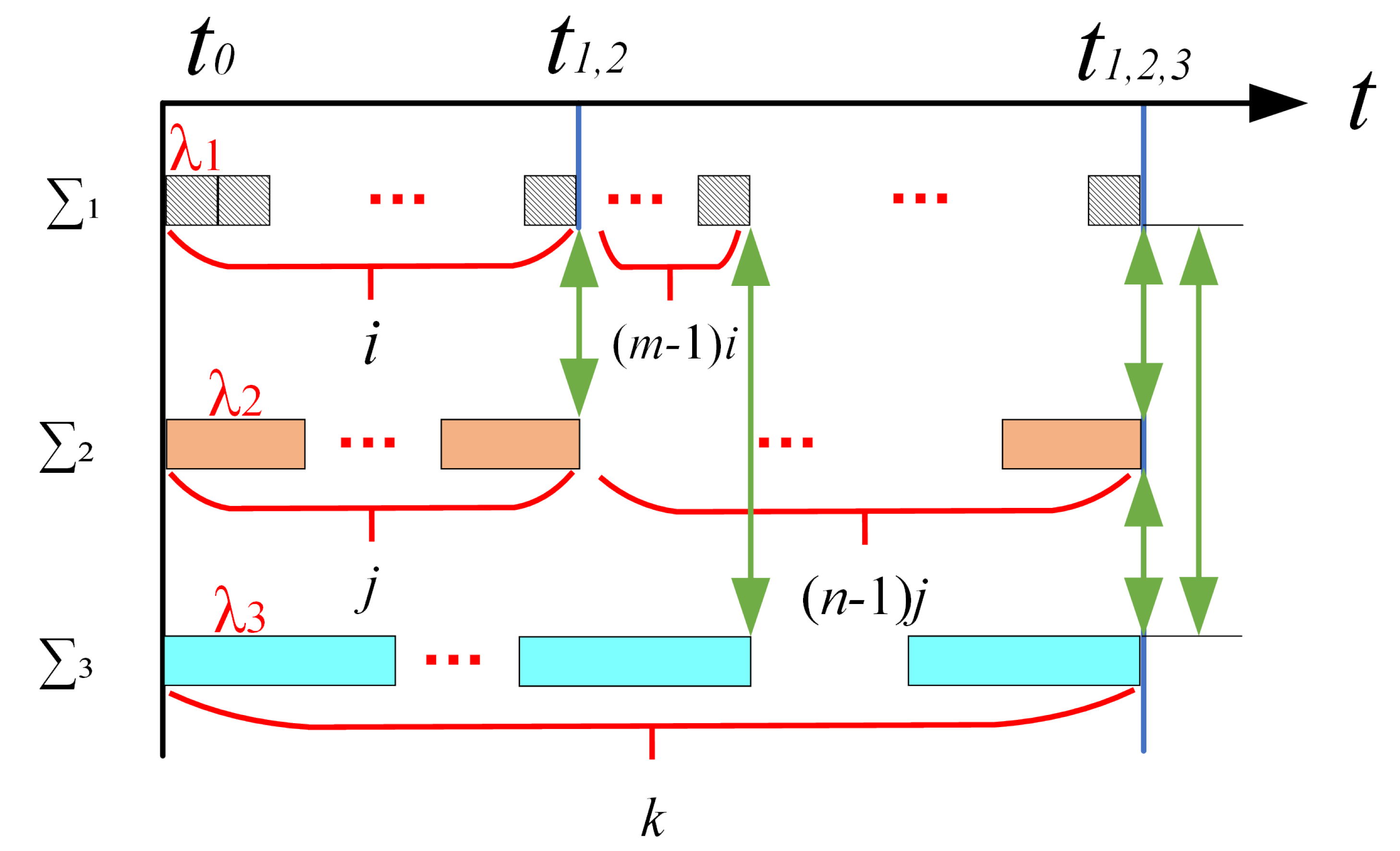
In this paper, a multi-scale time simulation approach compatible with different simulation step sizes is adopted. During simulation, different individuals may run independently for several time intervals and individual behaviors are executed in parallel; the value of the coupling variables are exchanged at a defined logic time called a macro-time step (MTS) [44]. After pushing one MTS, an output variable will be sent to the individual that has input with the same name. A different time step may be adopted internally, called a micro-time step ( μ TS). The synchronous method is explained by Figure 2. Taking three individuals 1 , 2 , 3 with different simulation step sizes λ 1 , λ 2 , λ 3 , all individuals initialize their logic time at t 0 . The first interaction occurs between 1 and 2 at t 1 , 2 when 1 has pushed i steps and 2 has pushed j steps. Thus, t 1 , 2 = i λ 1 = j λ 2 . Regarding t 1 , 2 , 3 , three individuals interact with one another, and 2 and 3 have pushed n , k steps, respectively. Here, t 1 , 2 , 3 is the lowest common multiple of λ 1 , λ 2 , λ 3 , and t 1 , 2 , 3 = n i λ 1 = n j λ 2 = k λ 3 .
The mathematical expression of the interaction time ( T ) for any two individuals the step sizes of which are λ and λ , respectively, is the following (Equation (6)):
T = { t | t % λ = 0 & t % λ = 0 } .

4. Implementation

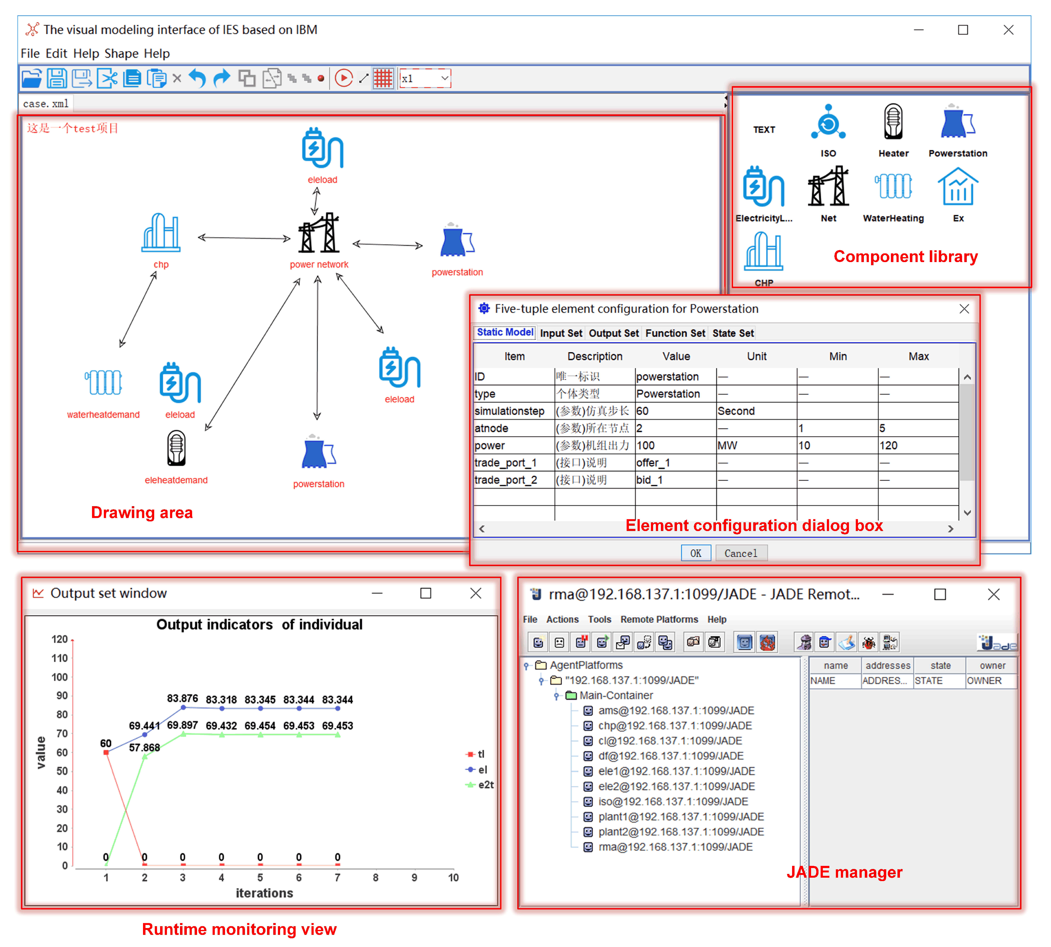
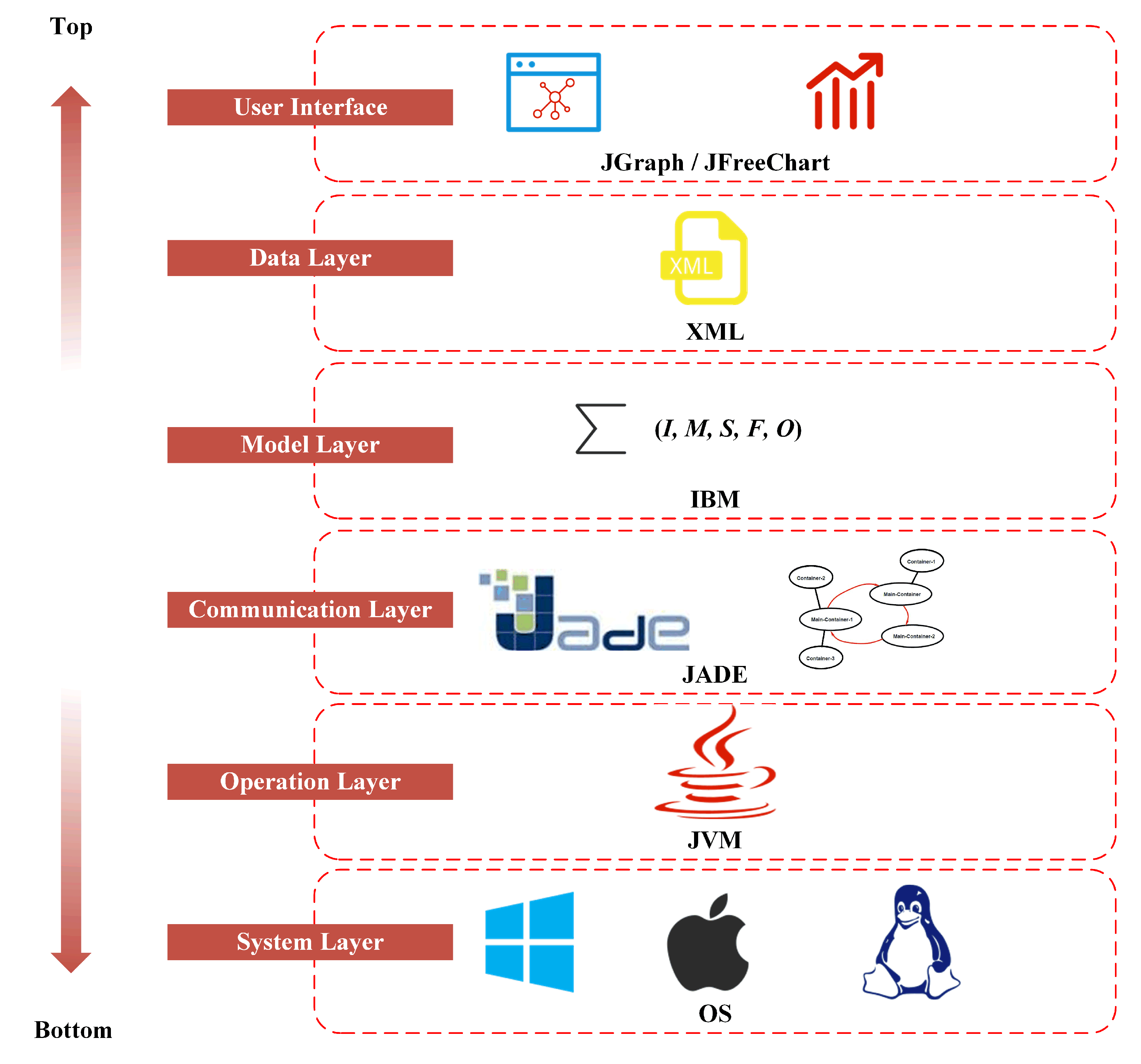
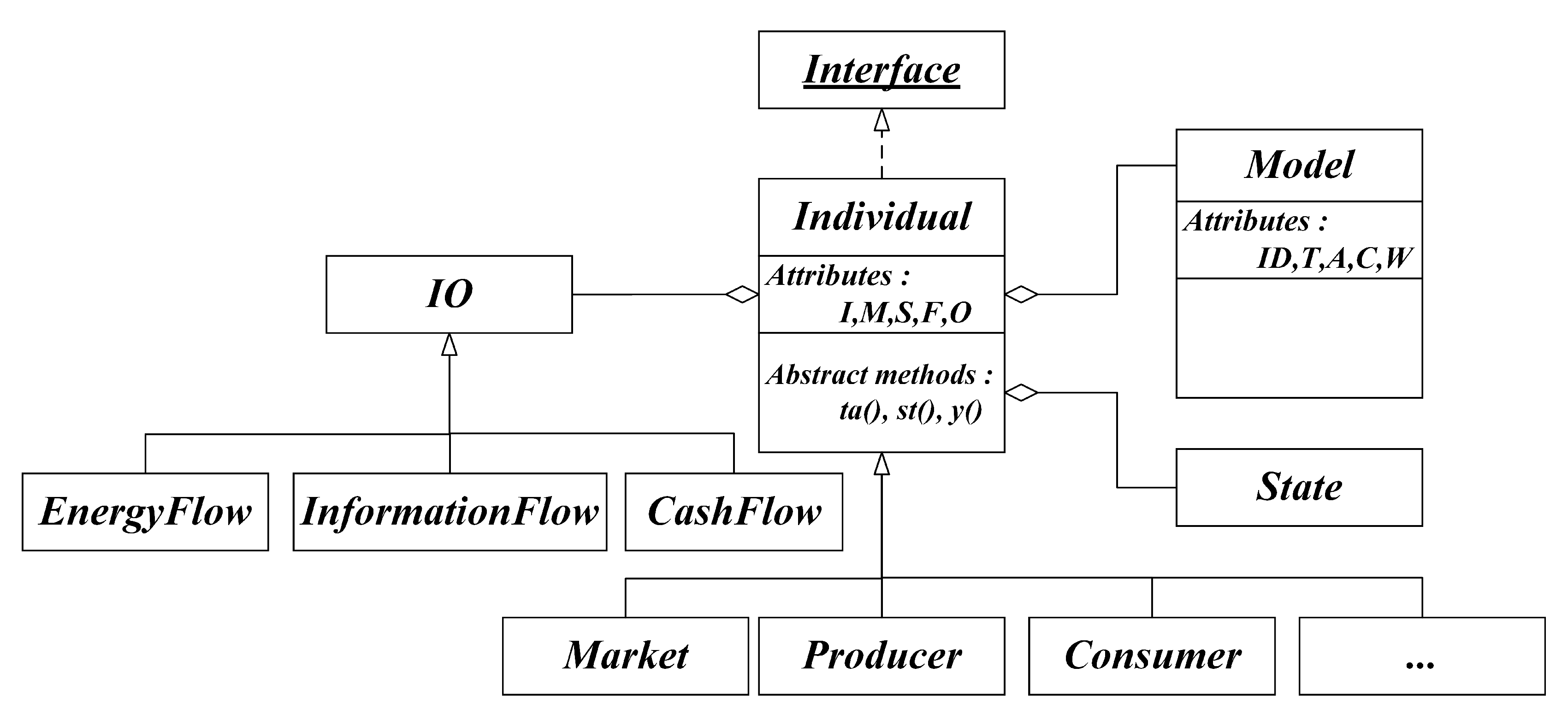
As shown in Figure 3, the proposed simulator is implemented with a hierarchical framework adopting Java, an object-oriented programming language. In this way, polymorphism and inheritance techniques can be used to realize reuse and extension. A Java virtual machine (JVM) is located between the operating system (OS) and Java agent development framework (JADE). This feature enables the emulator to function across platforms. JADE plays a role of communication between individuals and is located in the communication layer. Based on the IBM definition and object-oriented programming practice, the unified modeling language (UML) class diagram of the extensible IBM is presented as Figure 4. Extensible markup language (XML) is adopted for data modeling considering its standard and extensible form of expression. For the sake of individual-based simulation, component modeling can be implemented by visual interface actions such as dragging, dropping, and linking, with the help of third-party libraries such as JGraph [45]. It should be noted that JGraph is implemented on the basis of the model–view–controller architecture so that the model can be filled with the IBM directly without additional efforts. JFreeChart is an open charting class library on the Java platform, and with its help many kinds of charts can be generated, so that individual internal state and input or output indicators can be viewed. The visual modeling interface consists of five main panels, including the graphical modeling panel, component library, five-tuple configuration dialog, run monitor interface, and JADE manager. Among these panels, frequently used models are built into the component library panel, which can be added to the graphical modeling panel. In addition, the five-tuple configuration dialog provides an interface for setting up IBM data. The run monitor and JADE manager interface are responsible for individual indicator monitoring and JADE communication management, respectively.
Compared with other simulation platforms (mainly centralized standalone platforms), the proposed simulation platform can run on multiple hosts in a distributed manner, based on the above design and implementation methods. This can reduce performance requirements (such as memory and central processing unit) on a single machine. Based on experience, researchers can distribute the computational load of the system evenly across multiple hosts. In particular, we encourage researchers to take full advantage of multithreading and parallelism, which is supported by the simulation platform designed in this paper. The benefits are reflected in two aspects, one is different individuals can take up a thread to carry a task. Another is individual inner can also deal with parallel behavior. At the same time, the simulation times on different computers are synchronized according to the method in Section 3, to maintain the consistency of simulation times.

5. Case Study

Energy–economy coupled scenarios can be explored by building a series of IBMs that contains goals or constraints of a system individual. A scenario is introduced in this section to further clarify the application of the proposed model and method. The experiments were performed using a mid-range consumer laptop (Intel i5, 1.8 HZ and 8 G memory) to run the code and the visual interface, which also functioned as a data-logger.
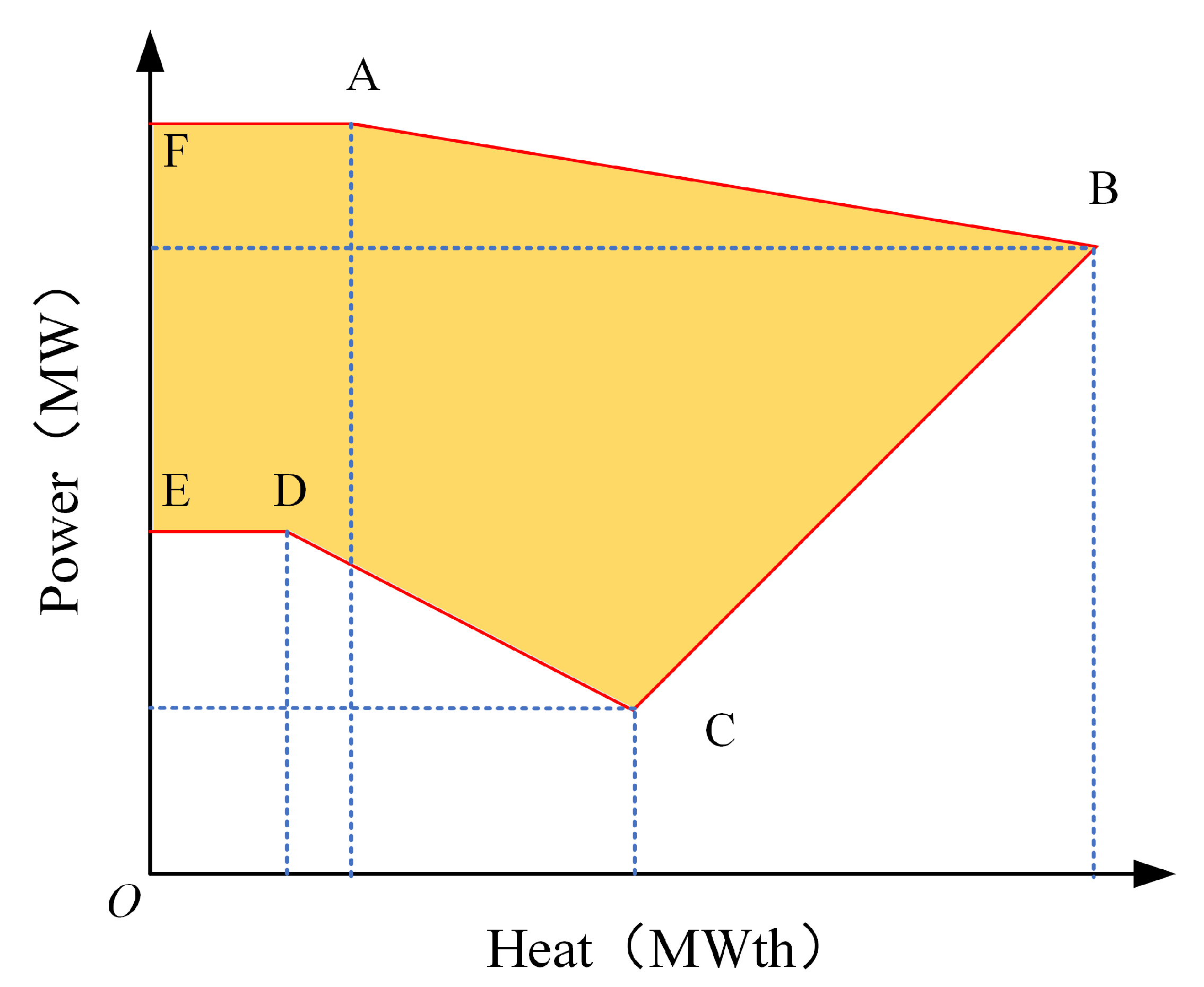
As shown in Figure 5, based on data presented in [46] and a modified IEEE three-machine system, a test system was conceived and outlined that contains heating and electricity. It is assumed that a co-generator ( G 2 ) is located at bus 2 ( B 2 ) and another two routine generators ( G 1 and G 3 ) are located at buses 1 and 3, respectively. G 2 provides a heating stream for the comprehensive load ( L 1 ) at bus 4 ( B 4 ) through a hot water pipeline without considering transmission loss. Figure 6 shows the thermal and electrical output feasible region of G 2 , which is described as a polygon [46]. In addition, G 1 and G 3 only provide the system with electricity. Regarding energy consumption, the consumer at B 4 is a comprehensive consumer having both heating and electrical demands. What needs to be illustrated here is that the heating demand can be met by water-heat radiators and an electric heater. Therefore, L 1 at B 4 must decide the volume of heating and electricity ( d t , L 1 h , d t , L 1 e ) to be purchased according to the published locational marginal price ( p t , L 1 e ) and preset heating price, as well as its maximized utility function (Equation (9)). Parameters μ h , μ e , σ h , and σ e in Equation (9) are coefficients of heating and the electricity utility function, respectively. v t , i h , v t , i and v t are decision variables, and k is the efficiency of the electric heater. d t , L 1 e consists of two parts: demand of non-heating electrical load ( d t , L 1 ) and demand of the electric heater ( d t , L 1 ). Therefore, total electrical demand d t , L 1 e = d t , L 1 + d t , L 1 for L 1 . The load at bus 5 ( L 2 ) and bus 6 ( L 3 ) are purely non-heating electricity loads.
At the beginning of the tth iteration, L 1 informs G 2 of its heating stream demands ( d t , L 1 h ). G 2 operates in the “electricity follows heating” mode to meet heating demand with adequate supply. Then, all of the loads submit their demands to the independent system operator (ISO) while generators report their marginal linear supply curve [47]. ISO performs the economical dispatch based on the optimal direct current flow and returns clearing results to each individual. Directly after that, each load individual participates in a new round of market and repeats the cycle according to the clearing price ( p t , L i e ). Similarly, all generators formulate their supply curve based on the clearing volume ( v t , G i e ).
Usually, the cost of a co-generator (e.g., c G 2 ) can be expressed as a multinomial of Equation (7), in which a 0 , a 1 , a 2 , a 3 , a 4 , and a 5 represent coefficients of cost. In this paper, a 0 = 2650 , a 1 = 14.5 , a 2 = 4.2 , a 3 = 0.0345 , a 4 = 0.03 , and a 5 = 0.031 . Letting v t h = 0 represent the cost of a traditional generator (i.e., G 1 and G 3 ), one can arrive at the marginal cost of electricity production of G 2 , i.e., (8), as well as its supply curve, Equation (11):
c G 2 = a 5 v t , G 2 e d t , L 1 h + a 4 ( d t , L 1 h ) 2 + a 3 ( v t , G 2 e ) 2 + a 2 d t , L 1 h + a 1 v t , G 2 e + a 0 ,
c G 2 = a 5 v t h + 2 a 3 v t e + a 1 ,
arg max ( v t , L 1 h , v t , L 1 , v t , L 1 ) 1 2 μ h v t , L 1 h + k v t , L 1 2 1 2 μ e v t , L 1 2 + σ h v t , L 1 h + k v t , L 1 + σ e v t , L 1 p t , L 1 h v t , L 1 h p t , L 1 e v t , L 1 + v t , L 1 .
The utility functions of L 2 and L 3 are given by the following formulation (Equation (10)):
arg max v t , L i e 1 2 μ e v t , L i e 2 + σ e v t , L i e p t , L i e v t , L i e ,
a t , G 1 = a 5 v t h + a 1 b t , G 1 = 2 a 3 p m i n = min { y | ( v t h , y ) R } p m a x = max { y | ( v t h , y ) R } ,
N = 2 6 550 0.072 3 6 240 0.101 2 4 240 0.161 3 5 240 0.170 4 1 240 0.085 5 1 240 0.092 .
The IBMs of the simulation case are listed in Table 2, in which R is the output feasible region of G 2 and N is the power network topology matrix, which is represented by a matrix as Equation (12). Each row of the matrix represents branch information of the transmission line, and the four columns of data represent the start bus number, end bus number, capacity, and reactance of the line, from left to right. E H , E L , and W H represent electric heater individual, electricity load individual, and water-heat radiators individual, respectively. N is the power network individual. WAIT and DECISION in the table means two finite states of the individual. WAIT & DECISION in the table means two finite states of the individual. p m i n   a n d   p m a x are the generator’s maximum and minimum generating capacity, respectively.
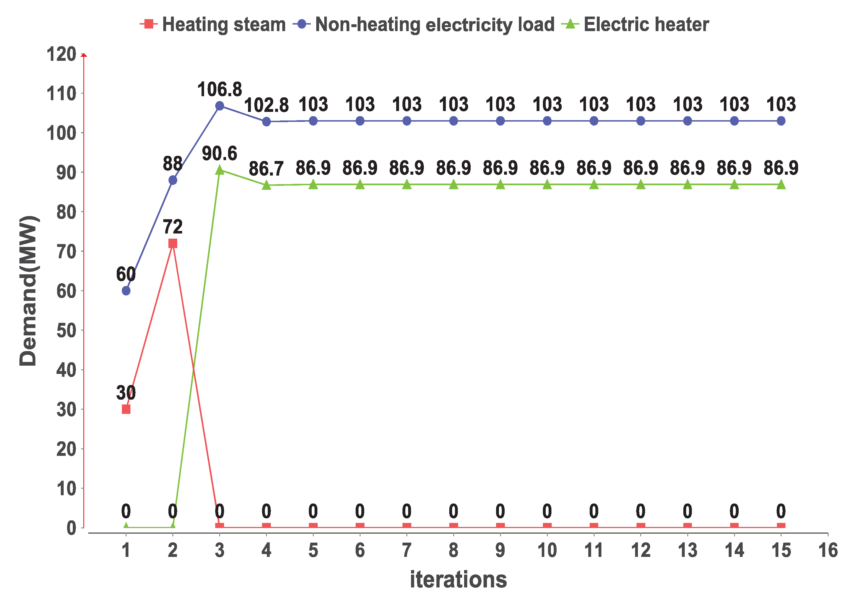
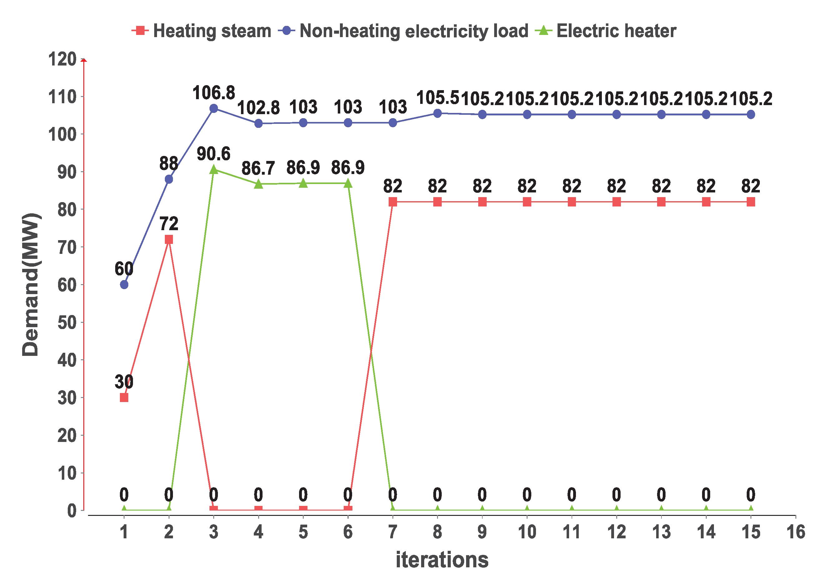
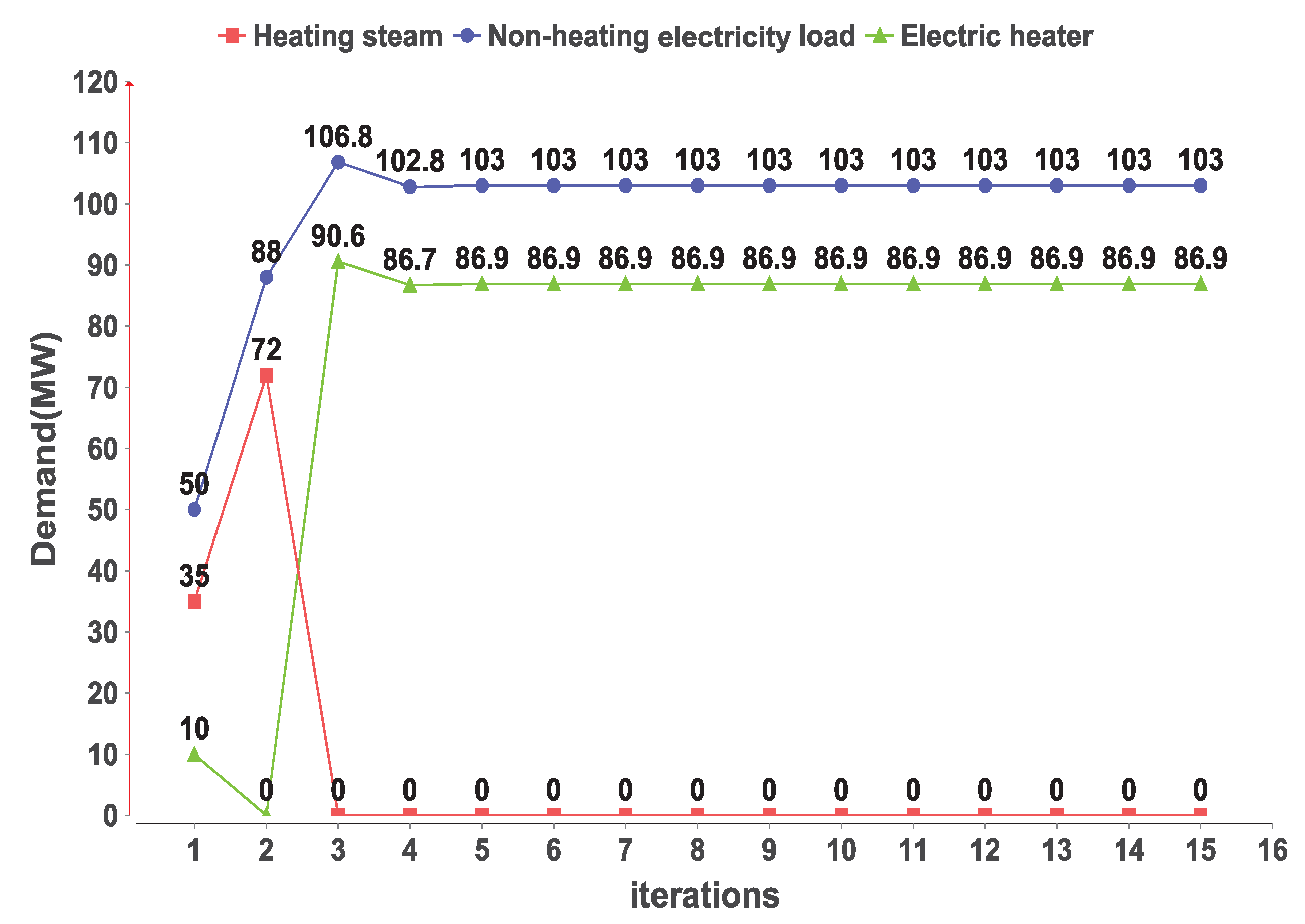
It is easy to see that the IBMs in Table 2 have the same data structure and interfaces and require only minor modifications. This will make it possible to reuse the model, greatly reducing the modeling effort. Figure 7 shows demand volume of comprehensive consumers for each delivery cover, including heating steam, non-heating electricity load, and electric heater. As can be seen in the figure, non-heating electricity load reaches up to the high value of 106.8 MW at the third iteration. Then, a drop occurs, followed by a slight rise from 102.8 to 103.0 MW. Upon changing the steam price from 21.0 to 18.0 $/MWh, it is seen that a low electricity price leads to more electricity purchased for electricity consumption and replacement, as shown in Figure 8. Because of the coupling of power and heat by the co-generator, the electrical consumption demand has also changed. It is necessary to note that 30.0, 60.0, and 0.0 MW were set as the initial values for v t , G 1 h , v t , G 1 , and v t , G 1 , respectively. When the initial values were changed to 35.0, 50.0, and 10.0 MW, a steady state is realized in a few iterations, as shown in Figure 9. As shown in Figure 9, we changed the initial demand value without changing the steam price and found that the system reached the same equilibrium after several iterations, indicating that the same equilibrium value can be obtained from different initial values. This is consistent with the common knowledge of research in this field. To a certain extent, it verified the effectiveness of the simulation model and method.
Compared to the centralized modeling approach, the IBM approach requires several interactions to reach equilibrium and may have a relatively inefficient optimization process or result because it does not have sufficient global information. At the same time, it is difficult to verify the high complexity problem mathematically. However, the distributed evolution process is still considered in the existing research to be a more realistic reflection of the dynamic process in the real world.

6. Conclusions

To summarize, considering the characteristics and requirements of the simulation of the EECS, this study obtained a suited IBM by defining standardized structures and elements. Following the bottom-up modeling idea, the IBM can be used to model each and every individual, no matter how complex or simple they are. In particular, it can work with multiple-timescale models, which is valuable for research on time-varying systems. Moreover, the reserved interface is an important feature of the IBM, which makes the IBM model more applicable, considering there is no universal algorithm for all individuals, both physical and social. In addition, a practical programming implementation method is developed that helps lower the threshold for beginners. According to the simulation case presented in this paper, the simulated target system can be represented by a regular and clear IBM set, which helps to reuse and globalize the model. In addition, the proposed method can describe the individual dynamic characteristics in the energy–economy coupled simulation scenario, and the simulation platform can clearly observe the dynamic process of the system. All these efforts aim to obtain a systematic approach that can help find better solutions for energy and environmental problems at the intersection of energy techniques, market economy, environmental protection, and human society. Although this work describes completion of the major portion of work in design and implementation, to show its significance, the model, method, and platform form a complete simulation architecture that is worthy of further improvement. At the same time, considering that the proposed method in this paper supports distributed simulation technology, it is valuable and promising to adopt a real complex system for modeling in our future research work.

Author Contributions

Conceptualization, J.Z. and Z.J.; software, J.Z.; validation, J.Z., Z.J., T.J. and N.A.L.; writing—original draft preparation, J.Z.; writing—review and editing, T.J. and N.A.L.; visualization, J.Z.; supervision, Z.J. All authors have read and agreed to the published version of the manuscript.

Funding

This work was supported by the State Key Program of the National Natural Science Foundation of China (Grant No. 51437006).

Conflicts of Interest

The authors declare no conflict of interest.

Appendix A

A hierarchical individual illustration is shown in Figure A1.
Figure A1. Hierarchical individual illustration.
Energies 13 02771 g0a1
The SWOT analysis matrix of the proposed method is shown in Table A1.
Table A1. The SWOT analysis matrix of the proposed method.
Strengths
1. Standardized and formalized model
2. Flexible time scale
3. Distributed and parallel
technologies inclusion
4. Dynamic simulation inclusion
Weaknesses
1. Difficult mathematical
theory validation
Opportunities
1. Distributed technologies are
in vogue
2. Interdisciplinary studies are
highly valued
3. Energy markets are being
implemented widely
4. Dynamic simulation is
considered to be more realistic
than pure centralization
mathematical optimization
Opportunity–Strength strategies
(use strengths to take advantage
of opportunities)
1. Standardized models can be used to
model multidisciplinary models uniformly
2. Multi-scale time simulation can adapt to
different models with different characteristics
3. It is promising to integrate distributed
frontiers, such as algorithms, models,
databases, and so on
4. Dynamic simulation is helpful to
understand the system characteristics
Opportunity–Weakness
strategies
(overcome weaknesses
by taking advantage of
opportunities)
1. Seeking support from
decentralized optimization
and game theory
Threats
1. The target system becomes
more and more complex
Threat–Strength strategies
(use strengths to avoid threats)
1. Decomposition modeling complex
systems based on individual model
2. Distributed parallel technology
can improve simulation performance
Threat–Weakness
strategies
(minimize weaknesses
and avoid threats)
1. Delimit boundaries of
the research and M&S
A visual modeling interface illustration is shown in Figure A2.
Figure A2. Simulator process visual modeling interface.
Energies 13 02771 g0a2

References

  1. Chen, X.; Mcelroy, M.; Wu, Q.; Shu, Y.; Xue, Y. Transition towards higher penetration of renewables: An overview of interlinked technical, environmental and socio-economic challenges. J. Mod. Power Syst. Clean Energy 2019, 7, 1–8. [Google Scholar] [CrossRef] [Green Version]
  2. Loulou, R.; Labriet, M. ETSAP-TIAM: The TIMES integrated assessment model Part I: Model structure. Comput. Manag. Sci. 2008, 5, 7–40. [Google Scholar] [CrossRef]
  3. Loulou, R.; Goldstein, G.; Noble, K. Documentation for the MARKAL Family of Models. Available online: http://www.iea-etsap.org/MrklDoc-III_SAGE.pdf (accessed on 26 May 2020).
  4. Connolly, D.; Lund, H.; Mathiesen, B.V.; Leahy, M. A review of computer tools for analysing the integration of renewable energy into various energy systems. Appl. Energy 2010, 87, 1059–1082. [Google Scholar] [CrossRef]
  5. Lopion, P.; Markewitz, P.; Robinius, M.; Stolten, D. A review of current challenges and trends in energy systems modeling. Renew. Sustain. Energy Rev. 2018, 96, 156–166. [Google Scholar] [CrossRef]
  6. Tesfatsion, L.; Judd, K. A Constructive Approach to Economic Theory in: Handbook of Computational Economics: Agent-Based Computational Economics; Elsevier Science: Amsterdam, The Netherlands, 2006. [Google Scholar]
  7. Robert, A.; Leigh, T. On-Line Guide for Newcomers to Agent-Based Modeling in the Social Sciences. Available online: http://www2.econ.iastate.edu/tesfatsi/abmread.htm (accessed on 8 April 2019).
  8. Wu, D.; Ning, S. Dynamic assessment of urban economy-environment-energy system using system dynamics model: A case study in Beijing. Environ. Res. 2018, 164, 70–84. [Google Scholar] [CrossRef]
  9. Vincenot, C.E. How new concepts become universal scientific approaches: Insights from citation network analysis of agent-based complex systems science. Proc. Biol. Sci. 2018, 285, 20172360. [Google Scholar] [CrossRef]
  10. Basu, N.; Pryor, R.; Quint, T. ASPEN: A Microsimulation Model of the Economy. Comput. Econ. 1998, 12, 223–241. [Google Scholar] [CrossRef]
  11. Li, H.; Leigh, T. The AMES Wholesale Power Market Test Bed: A Computational Laboratory for Research, Teaching, and Training. In Proceedings of the 2009 IEEE Power & Energy Society General Meeting, Calgary, AB, Canada, 26–30 July 2009. [Google Scholar]
  12. De Coninck, R.; Baetens, R.; Verbruggen, B.; Driesen, J.; Saelens, D.; Helsen, L. Modelling and simulation of a grid connected photovoltaic heat pump system with thermal energy storage using Modelica. In Proceedings of the 8th International Conference on System Simulation in Buildings, Belgium, Liege, 13–15 December 2010; p. 177. [Google Scholar]
  13. Ghersi, F. Hybrid bottom-up/top-down energy and economy outlooks: A review of IMACLIM-S experiments. Front. Environ. Sci. 2015, 3. [Google Scholar] [CrossRef] [Green Version]
  14. Schweiger, G.; Gomes, C.; Engel, G.; Hafner, I.; Nouidui, T. An Empirical Survey on Co-simulation: Promising Standards, Challenges and Research Needs. Simul. Model. Prac. Theory 2019, 95. [Google Scholar] [CrossRef] [Green Version]
  15. Deane, J.; Chiodi, A.; Gargiulo, M.; Gallachóir, B.P. Soft-linking of a power systems model to an energy systems model. Energy 2012, 42, 303–312. [Google Scholar] [CrossRef]
  16. Energy Exemplar, PLEXOS for Power Systems. Available online: http://www.energyexemplar.com (accessed on 8 April 2019).
  17. Loulou, R.; Remme, U.; Kanudia, A.; Lehtilä, A.; Goldstein, G. Documentation for the TIMES model. Available online: https://www.researchgate.net/publication/242686300_Documentation_for_the_TIMES_model (accessed on 27 May 2020).
  18. Martín-Lopo, M.M.; Boal, J.; Sánchez-Miralles, Á. Transitioning from a meta-simulator to electrical applications: An architecture. Simul. Model. Pract. Theory 2019, 94, 177–198. [Google Scholar] [CrossRef]
  19. E3MLab. PRIMES Model—Detailed Model Description (Version 2018). Available online: http://www.e3mlab.eu/ (accessed on 8 April 2019).
  20. Becker, D.; Saxton, T.L. CIM standard for model exchange between planning and operations. In Proceedings of the 2008 IEEE Power and Energy Society General Meeting-Conversion and Delivery of Electrical Energy in the 21st Century, Pittsburgh, PA, USA, 20–24 July 2008; pp. 1–5. [Google Scholar] [CrossRef]
  21. Electronic Data Interchange Library. Available online: https://www.entsoe.eu/publications/electronic-data-interchange-edi-library/ (accessed on 8 April 2018).
  22. Odell, J.; Giorgini, E.A. Agent-Oriented Software Engineering V; Springer: Berlin/Heidelberg, Germany, 2004. [Google Scholar] [CrossRef]
  23. Granado, P.C.D.; Van Nieuwkoop, R.; Kardakos, E.G.; Schaffner, C. Modelling the energy transition: A nexus of energy system and economic models. Energy Strategy Rev. 2018, 20, 229–235. [Google Scholar] [CrossRef] [Green Version]
  24. Wei, W.; Wu, D.; Wu, Q.; Shafie-Khah, M.; Catalao, J.P.S. Interdependence between transportation system and power distribution system: A comprehensive review on models and applications. J. Mod. Power Syst. Clean Energy 2019, 7, 433–448. [Google Scholar] [CrossRef] [Green Version]
  25. Grimm, V.; Railsback, S.F. Individual-Based Modeling and Ecology; Princeton University Press: Princeton, NJ, USA; Oxford, UK, 2005. [Google Scholar] [CrossRef]
  26. Grimm, V.; Berger, U.; Bastiansen, F.; Eliassen, S.; Ginot, V.; Giske, J.; Goss-Custard, J.; Grand, T.; Heinz, S.K.; Huse, G. A standard protocol for describing individual-based and agent-based models. Ecol. Model. 2006, 198, 115–126. [Google Scholar] [CrossRef]
  27. Grimm, V.; Berger, U.; DeAngelis, D.L.; Polhill, J.G.; Giske, J.; Railsback, S.F. The ODD protocol: A review and first update. Ecol. Model. 2010, 221, 2760–2768. [Google Scholar] [CrossRef] [Green Version]
  28. Wang, L.; Zheng, J.; Li, M.; Lin, X.; Jing, Z.; Wu, P.; Wu, Q.; Zhou, X. Multi-time scale dynamic analysis of integrated energy systems: An individual-based model. Appl. Energy 2019, 237, 848–861. [Google Scholar] [CrossRef]
  29. Energy Modeling Framework: Model for Energy Supply Strategy Alternatives and Their General Environmental Impact (MESSAGE). International Institute for Applied Systems Analysis (IIASA). Available online: https://webarchive.iiasa.ac.at/Research/ENE/model/message.html (accessed on 15 May 2020).
  30. Enerdata. POLES: Prospective Outlook on Long-Term Energy Systems. Available online: https://www.enerdata.net/solutions/poles-model.html (accessed on 15 May 2020).
  31. KTH—Division of Energy System Analysis. OSeMOSYS Documentation (Release 0.0.1). Available online: https://osemosys.readthedocs.io/_/downloads/en/latest/pdf/ (accessed on 15 May 2020).
  32. Stockholm Environment Institute. Long Range Energy Alternatives Planning (LEAP) System. Available online: https://www.energycommunity.org/default.asp (accessed on 15 May 2020).
  33. Fishbone, L.G.; Abilock, H. Markal, a linear-programming model for energy systems analysis: Technical description of the bnl version. Int. J. Energy Res. 1981, 5, 353–375. [Google Scholar] [CrossRef]
  34. Messner, S.; Golodnikov, A.; Gritsevskii, A. A stochastic version of the dynamic linear programming model MESSAGE III. Energy 1996, 21, 775–784. [Google Scholar] [CrossRef] [Green Version]
  35. Kitous, A. POLES Description. Available online: http://www.yegm.gov.tr/projeler/document/5_POLES_description.pdf (accessed on 16 May 2020).
  36. Howells, M.; Rogner, H.; Strachan, N.; Heaps, C.; Huntington, H.; Kypreos, S.; Hughes, A.; Silveira, S.; DeCarolis, J.; Bazillian, M.; et al. OSeMOSYS: The Open Source Energy Modeling System: An introduction to its ethos, structure and development. Energy Policy 2011, 39, 5850–5870. [Google Scholar] [CrossRef]
  37. Stockholm Environment Institute. Model for Energy Supply Strategy Alternatives and their General Environmental Impact (MESSAGE). Available online: https://www.energyplan.eu/othertools/global/message/ (accessed on 15 May 2020).
  38. KTH Royal Institute of Technology. Development of the Model Management Infrastructure (MoManI) Interface. Available online: https://www.energy.kth.se/energy-systems/completed-projects/development-of-the-model-management-infrastructure-momani-interface-1.940019 (accessed on 15 May 2020).
  39. International Academy of Mathematical Chemistry. Model Concept, Solver and Details—POLES. Available online: https://www.iamcdocumentation.eu/index.php/Model_concept,_solver_and_details_-_POLES (accessed on 16 May 2020).
  40. OSeMOSYS Official Website. OSeMOSYS Code. Available online: http://www.osemosys.org/get-started.html (accessed on 15 May 2020).
  41. Hilpert, S.; Kaldemeyer, C.; Krien, U.; Günther, S.; Wingenbach, C.; Plessmann, G. The Open Energy Modelling Framework (oemof)—A new approach to facilitate open science in energy system modelling. Energy Strategy Rev. 2018, 22, 16–25. [Google Scholar] [CrossRef] [Green Version]
  42. Parrott, L. Hybrid modelling of complex ecological systems for decision support: Recent successes and future perspectives. Ecol. Inform. 2011, 6, 44–49. [Google Scholar] [CrossRef]
  43. Vincenot, C.E.; Mazzoleni, S.; Parrott, L. Editorial: Hybrid Solutions for the Modeling of Complex Environmental Systems. Front. Environ. Sci. 2016, 4, 53. [Google Scholar] [CrossRef] [Green Version]
  44. Molitor, C.; Groß, S.; Zeitz, J.; Monti, A. MESCOS—A Multienergy System Cosimulator for City District Energy Systems. IEEE Trans. Ind. Inform. 2014, 10, 2247–2256. [Google Scholar] [CrossRef] [Green Version]
  45. JGraph Specialises in Browser-Based Diagramming Components and Applications. Available online: https://github.com/jgraph (accessed on 8 April 2019).
  46. Tao, G.; Henwood, M.; van Ooijen, M. An algorithm for combined heat and power economic dispatch. IEEE Trans. Power Syst. 2002, 11, 1778–1784. [Google Scholar] [CrossRef]
  47. Li, H.; Sun, J.; Leigh, T. Dynamic LMP response under alternative price-cap and price-sensitive demand scenarios. In Proceedings of the 2008 IEEE Power and Energy Society General Meeting, Pittsburgh, PA, USA, 20–24 July 2008; pp. 1–8. [Google Scholar] [CrossRef]
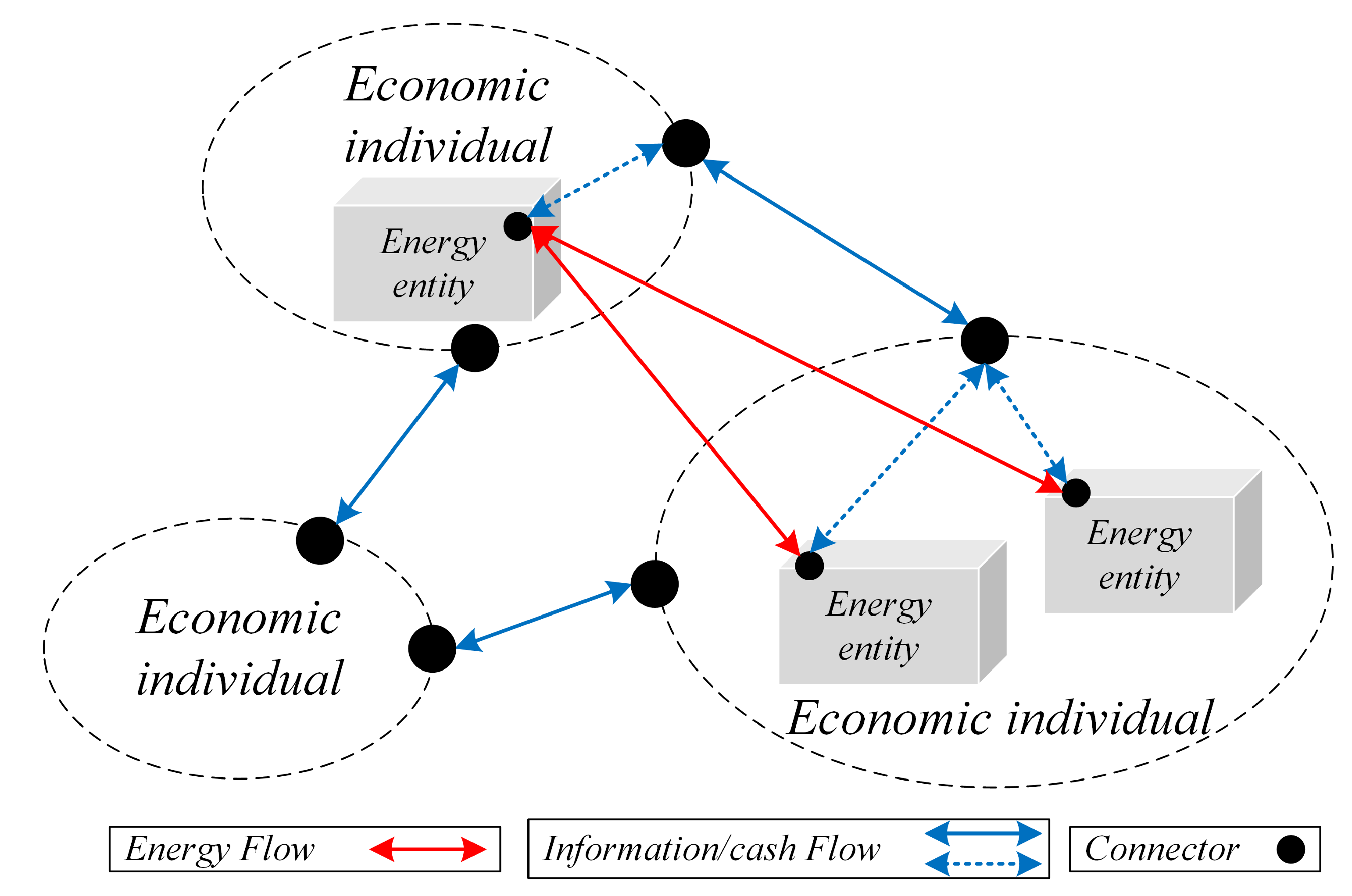
Figure 1. Multiple individuals with different types and sizes in energy system.
Energies 13 02771 g001
Figure 2. Individual interaction moments with different simulation step sizes.
Energies 13 02771 g002
Figure 3. Simulator hierarchical framework.
Energies 13 02771 g003
Figure 4. UML class diagram of IBM.
Energies 13 02771 g004
Figure 5. Topology of test system.
Energies 13 02771 g005
Figure 6. Co-generator heat-power output feasible region: A (32.4, 125.8); B (135.6, 110.2); C (75, 40); D (15.9, 44), E (0, 44); and F (0, 125.8).
Energies 13 02771 g006
Figure 7. Dynamic equilibrium is reached after several iterations.
Energies 13 02771 g007
Figure 8. When the steam price changes after the sixth iteration, the mix of energy demand changes.
Energies 13 02771 g008
Figure 9. Dynamic equilibrium is still reached, even if the setting of the initial value has changed.
Energies 13 02771 g009
Table 1. The feature comparison of various modeling and simulation methods in the energy economy field.
MARKAL (MARKet Allocation Model) [3]MESSAGE (Model for Energy Supply Strategy Alternatives and Their General Environmental Impact) [29]PRIMES (Price-Induced Market Equilibrium System) [19]POLES (Prospective Outlook on Long-Term Energy Systems) [30]OSeMOSYS (Open Source Energy Modelling System) [31]LEAP (Long-Range Energy Alternatives Planning System) [32]The Proposed Method
MethodologyBottom-upBottom-upHybridHybridBottom-upHybridBottom-up
Model classification Mathematical programming [33]Mathematical programming [34]SimulationEconometric [35]Mathematical programmingAccountingSimulation
Model scope Energy sector onlyEnergy sector onlyEuropean energy sector and its market [19]Mainly energy supply and demand sectorsEnergy sectorEnergy and climate sectorEnergy economy system
Dynamic simulation UnsupportedUnsupportedSupportedSupportedSupportedUnsupportedSupported
Model standardization PersonalizedPersonalizedPersonalizedPersonalizedPersonalized [36]PersonalizedFormalization
Privacy protection PoorPoorGoodPoorPoorPoorGood
Time horizon Medium, long termMedium, long term [37]Long term up to 2070Up to 2050 [30]Long termMedium, long termShort, medium, long term
Time step User-defined5 or 10 years [37]YearlyYearlyYearlyYearlyUser-defined
Interaction method Hard-linkedSoft- and hard-linkedSoft-linkedHard-linkedHard-linkedUnknownSoft-linked
Distributed or parallel technology UnsupportedUnsupportedUnsupportedUnsupportedUnknownUnsupportedSupported
VisualizationUnknownUnknownUnsupportedUnsupportedUnsupported but the third part interface available [38]SupportedSupported
Language or software GAMS [3]FORTRAN [29]UnknownVensim software required [39]MathProg and being translated into GAMS and Python [40]MathProgJAVA/JADE
ScalabilityOrdinaryOrdinaryGoodOrdinaryGood [31]OrdinaryGood
Interaction method: a coupling of existing models (“soft-linked”) or a single integrated model which blends features of both top-down and bottom-up models (“hard-linked”).
Table 2. Individual model elements.
L 1 L i ( i = 2 , 3 ) G i ( i = 1 , 3 ) G 2 O
I p t , L 1 h , p t , L 1 e p t , L i e v t , G i e d t , 1 h , v t , G 2 e a t , G i , b t , G i , d t , L i e ,
p m a x , p m i n
ID L i L 2 G i G 2 O
TComprehensive ConsumerConsumerGeneratorCo-generatorISO
MA μ h , μ e , σ h , σ e , k μ e , σ e P m i n i , P m a x i R N
C C G 2 , C O C O C O C O , C L 1 C L i , C G i
W E H , E L , W H N
S WAIT , DECISION WAIT , DECISION WAIT , DECISION WAIT , DECISION WAIT , DECISION
FEquation (9)Equation (10)Equations (8) and (11) and v t h = 0 Equations (8) and (11) min i = 1 3 c G i
O d t , 1 h , d t , 1 e d t , i e a t , G i , b t , G i a t , G 2 , b t , G 2 ,
p m a x , p m i n
v t , i e , p t , i e