Multi-Objective Tabu Search for the Location and Sizing of Multiple Types of FACTS and DG in Electrical Networks

Abstract

Flexible AC transmission systems and distributed generation units in power systems provide several benefits such as voltage stability, power loss minimization, thermal limits enhancement, or enables power system management close to the limit operation points; and by extension, economic benefits such as power fuel cost and power loss cost minimization. This work presents a multi-objective optimization algorithm to determine the location and size of hybrid solutions based on a combination of Flexible AC transmission systems devices and distributed generation. Further, the work expands the types of FACTS usually considered. The problem is solved by means of a Tabu search algorithm with good results when tested in a network of 300 nodes.

1. Introduction

In deregulated markets, power transactions in transmission and distribution networks lead the power systems to operate close to their limits to maximize the benefits [1,2,3,4]. Furthermore, climate change and other environmental concerns force the installation of distributed generation (DG) units, renewable and conventional, close to load centres to feed the demand growth [5]. There is no doubt that the installation of DG has benefits for both the consumer, the supplier and the network [6], but the increase in the penetration of the DG can also cause several problems in the operation of the network [7] (voltage profile, stability, wave quality, harmonics, imbalances, …). The creation of a microgrid architecture [8] together with a suitable energy management system [9] is the most advantageous mode of operation for both the consumer and the network.

Flexible AC transmission systems (FACTS) and DG installations in the transmission lines have the capacity to enhance power systems [10]. However, finding the optimal FACTS and DG devices location for power system enhancement is a non-linear complex problem which involves economical, environmental and electrical variables. In the technical literature, authors have used different FACTS to control the power network attributes [3,11,12] as summarized in

Table 1. FACTS control attributes.

FACTS Controller	Control Attributes
	1	2	3	4	5	6	7	8	9
STATCOM	x	x	x	x
SVC	x	x	x	x	x
SSSC			x		x	x	x
TCSC			x	x	x	x	x
UPFC	x	x	x	x	x		x	x	x

(1) Voltage control, (2) VAr compensation, (3) damping oscillations, (4) voltage stability, (5) transient and dynamic stability, (6) current control, (7) fault current limiting, (8) active power control, (9) reactive power control.

. Several authors utilise intelligent systems to improve the voltage stability in real time, during the operation of saturated electrical networks. Devaraj et al. [13] use a radial basis function network model to estimate the voltage stability level of the power system based on the L-index, and this way, detect how far the nodes are from voltage collapse. Tomin et al. [14] present an automatic intelligent system for voltage security control based on a decision trees model, and use the L-index for the localisation of critical nodes. Satheesh et al. [15] use a neural network to identify the optimal location of FACTS controllers and a Bees algorithm to calculate the operation point of these devices in the power system.

One way to solve the problem in consideration is by optimizing an economic objective function, formulated with fixed kVAr costs [16,17] or with quadratic formulations [18,19,20,21,22,23,24,25]. Other authors include the annual investment cost [26], capital recovery factor [27,28], annual cost device [29], or a combination of them; as well as the active power generation fuel cost and the reactive power generation fuel cost, if the DG units are combustion machines [30,31,32]. The optimization problem is usually subject to common power flow constraints, such as bus voltage limits, thermal limits, feeders power transfer capability, real and reactive power generation limits, among others [33,34].

Another way is to solve it as a multi-objective optimization problem and obtain a set of non-dominated solutions. Authors in [35] optimize the location of thyristor controlled series capacitors (TCSC) and/or static VAR compensators (SVC), considering the investment and power generation cost as objective functions, by means of genetic algorithms (GA), successive linear programming and Benders decomposition, maintaining the voltage profile within its limits. Another multi-objective formulation of FACTS costs has been developed by [36], averaging investment and generation costs, and solving with a GA technique to find the optimal location of unified power flow control (UPFC), TCSC, thyristor controlled phase shifting transformer and SVC devices in power systems, where the FACTS candidate nodes and lines are selected using a randomization method. Voltage profile enhancement and TCSC device number minimization are used as objectives to improve line congestion in [37], and solved through simulated annealing and sequential quadratic programming (SQP) algorithms. A model for finding the optimal location of TCSC and SVC devices using a hybrid GA-SQP algorithm with a fuzzy multi-objective function, that includes power loss, investment cost (quadratic costs functions), peak point power generation, voltage deviation, as well as security margin minimization, is presented by [38]; this work is addressed in [39], adding Pareto optimal solutions to obtain faster results. Other authors [40,41] determine the maximum loading factor possible, implementing FACTS devices in power systems, taking into account the voltage deviation and the real power loss minimization, finding the optimal parameters settings and locations of coordinated SVC and TCSC devices, and selecting the best compromise solution of the Pareto optimal solutions in non-dominated sorting particle swarm optimization. The optimal FACTS location problem is solved in [42] considering the power system total cost, where Akaike’s information criterion is minimized and the expected security is maximized. A multi-objective non-dominated sorting improved harmony search is proposed by [43] for voltage stability improvement, considering the optimal placement of TCSC and/or SVC devices in power systems through loading factor maximization, and voltage deviation and real power loss minimization. The gravitational search algorithm is introduced and compared with particle swarm optimization for reactive power planning, considering FACTS implementation in power systems, by [44]; in said work, the goal is to minimize both real power loss and FACTS investment cost, while increasing the reactive load. The effectiveness of the harmony search algorithm is used in [45] to find optimal TCSC and static synchronous series compensator (SSSC) locations, considering power system loading factor maximization.

Presently, Tabu search has been used in the location and sizing of DG [46] or the FACTS [47,48,49,50] with mono-objective models, and with multi-objective models for the location and sizing of DG [51]. In this paper, a multi-objective Tabu search (MOTS) algorithm is carried out to find the optimal location and size of FACTS devices and DG units in a power system network. The problem has also been generalized by expanding the types of FACTS considered, including their hybrid use with other solutions, such as the installation of DG and high-voltage direct current (HVDC) systems. The FACTS devices considered in this work are: HVDC, STATCOM, SSSC, SVC, TCSC and UPFC. Section 2 depicts the multi-objective function, and the tabu search algorithm method, including the description of the permanency and the recency effect in the memory, and the selection of nodes and branches through analytical methods. Section 3 presents the test results obtained for a modified IEEE 300-bus system. Finally, in Section 4 the conclusions are presented.

2. Methodology

In the proposed model, an analytical method is applied to select the lines or buses to install DG units or FACTS devices to enhance the power system stability, taking into consideration the technical power flow constraints and the total power system cost analysis. Costs are presented in annualized values, with the objective to obtain benefits regarding the total investment cost (TIC) and the total generation cost (TGC), including the power losses cost (PLC). The algorithm is coded in MATLAB 2019 using the continuation power flow routine extracted from the power system analysis toolbox [52] to work embedded with tabu search [53]. The results are compared with the initial solution on a IEEE 300 bus test system.

2.1. Cost Functions

The economic analysis in this work employs the $TIC$, the $TGC$, and the $PLC$. To calculate the $TIC$, maintenance, operation and installation costs are considered. For the $TGC$, reference bus active power generation cost ($PGC$), and DG units $PGC$ and reactive power generation cost ($QGC$) are taken into account.

2.1.1. Power Losses Cost

The $PLC$ is determined by the continuation power flow using the mathematical formulation presented in [54].

$$PLC=\sum _{pϵN_p}\sum _{ijϵN_L}P{l}_{ij,p}·C_{\mathrm{L},p}·{\alpha }_p^{\mathrm{PLC}}$$

(1)

where ${\alpha }_p^{\mathrm{PLC}}$ (Equation (2)) is the power loss discount rate for the $PLC$ determination in period p; $P{l}_{ij,p}$ are the power losses in the line $ij$ in period p; $C_{\mathrm{L},p}$ is the cost of losses in period p in $/kWh, $N_p$ is the period set and $N_L$ is the lines set.

The discount factors are determined by means of:

$${\alpha }_p^{\mathrm{PLC}}=\stackrel{ny}{\sum _{y=1}}\frac{{\left(1+L{G}_p\right)}^y}{{\left(1+r\right)}^{\left(ny\right)\left(p-1\right)+y}}$$

(2)

where $ny$ are the periods in the planning horizon in years; $L{G}_p$ is the load annual growth rate in period p; and r is the annual interest rate.

2.1.2. FACTS Costs

In this research, HVDC, TCSC, SSSC, STATCOM, SVC and UPFC are the devices considered to enhance the power system network, and thus, it is necessary to determine the FACTS investment cost (FIC).

$$FIC=\sum _{iϵN_F}\mathrm{CRF}·C_i$$

(3)

where $N_F$ is the FACTS set, the FACTS cost $\left(C_i\right)$ and the capital recovery factor (CRF) [27,28,29,55,56,57,58,59,60,61,62,63] are:

$$C_i=F_{1,i}·S_i^2-F_{2,i}·S_i+F_{3,i}$$

(4)

$$\mathrm{CRF}={\displaystyle \frac{r{\left(1+r\right)}^{ny}}{{\left(1+r\right)}^{ny}-1}}$$

(5)

where $S_i$ is the nominal apparent power of FACTS i.

The values of the coefficients $F_{1,i},F_{2,i}$ and $F_{3,i}$ are specified in

Table A1. Cost functions coefficients for FACTS devices.

Device	${\mathit{F}}_1$	${\mathit{F}}_2$	${\mathit{F}}_3$
HVDC	0.1576	711.9	26,330
TCSC	0.0015	−0.7130	153.75
STATCOM	0.0001	−0.185	158
SSSC	0.00039	−0.3245	173.42
SVC	0.0003	−0.3051	127.38
UPFC	0.0003	−0.2691	188.22

. These coefficients are retrieved from [18,19,20,21,22,23,24,25,64]. For the STATCOM function, the data curve recognition provided by [18] is employed; the values for the HVDC are obtained by adjusting the curve using the cost information calculated in [64].

2.1.3. Distributed Generation Costs

The DG units are considered as PV nodes and the costs are simulated as diesel generators. In [30,31,32,36,65,66,67], the simplified equation for $PGC$ is presented, taking into account the equations developed by [68].

$$PGC=8760·\left\{\left[\sum _{i\in N_{\mathrm{G}}}\left({\alpha }_{2,i}·P_{\mathrm{G},i}^2+{\alpha }_{1,i}·P_{\mathrm{G},i}+{\alpha }_{0,i}\right)\right]+61.38·P_{\mathrm{G},\mathrm{SW}}\right\}$$

(6)

where ${\alpha }_{2,i}$, ${\alpha }_{1,i}$ and ${\alpha }_{0,i}$ are the generators coefficients [57,62,69,70,71,72] (

Table A2. Coefficients for active power generation cost depending on their production capacity.

${\mathit{P}}_{\mathit{G},\mathit{i}}^{max}$	${\mathit{P}}_{\mathit{G},\mathit{i}}^{min}$	${\mathit{Q}}_{\mathit{G},\mathit{i}}^{max}$	${\mathit{P}}_{\mathit{G},\mathit{i}}^{min}$	${\mathit{\alpha }}_2$	${\mathit{\alpha }}_1$	${\mathit{\alpha }}_0$
MW	MW	MVAr	MVAr	$/MW2h	$/MWh	$/h
250	45	150	−100	0.000820	11.00	692.32
250				0.11000	5.00	150
250				0.12250	1.00	33
200				0.08500	1.50	0
150	15	50	−40	0.000776	12.00	692.32
118.9				0.07000	30.00	0
55				0.00830	3.25	0
30				0.02500	3.00	0
8.0				0.00040	24.30	0
3.6	0.5	1.5	−0.4	0.0037	2	18
3.0				0.00060	29.10	0
2.7	0.2	1.0	−0.8	0.01	10	100
2.5	0.2	0.8	−0.8	0.05	30	100
2.0	0.3	0.5	−0.5	0.02	15	100
2.0	0.2	0.8	−0.8	0.05	30	100
2.0	0.4	0.7	−0.7	0.03	20	100
2.0				0.00150	50.00	0
1.4	0.2	0.6	−0.4	0.0175	1	16
1.2				0.00067	6.90	0
1.0	0.15	0.4	−0.4	0.0625	1	14
1.0	0.10	0.4	−0.1	0.0083	3.25	12
1.0	0.10	0.24	−0.6	0.025	3	13
0.8				0.00026	6.90	0

); the coefficient 61.38 is obtained from [73]; $P_{\mathrm{G},i}$ is the active power supplied by generator i and $N_{\mathrm{G}}$ is the generators set.

The $QGC$ equations are developed in [65,74], where ${\beta }_{1,i}=0.1{\alpha }_{1,i}$ and ${\beta }_{0,i}=0.1{\alpha }_{0,i}$ [65]; and $Q_{\mathrm{G},i}$ is the reactive power supplied by generator i.

$$QGC=8760·\left[\sum _{i\in N_{\mathrm{G}}}\left({\beta }_1·Q_{\mathrm{G},i}+{\beta }_0\right)\right]$$

(7)

The distributed generation investment cost ($GIC$) function considers the CRF, DG installation cost, and operation and maintenance costs in the $C_i$ value [75].

$$GIC=\sum _{i\in N_{\mathrm{G}}}\mathrm{CRF}·C_i$$

(8)

2.1.4. Multi-Objective Function

The multi-objective function presented aims at minimizing the $TIC$ and the $TGC$, where the $TIC$ is formulated by means of the Equations (3) and (8). The $TGC$ is calculated using Equations (1), (6) and (7).

$$min\left(TGC\right)=min\left(PGC+QGC+PLC\right)$$

(9)

$$min\left(TIC\right)=min\left(FIC+GIC\right)$$

(10)

Subject to the following constraints:

-

Power balance with FACTS in each bus i:

$$P_i(\vartheta ,V)-P_{\mathrm{G},i}+P_{\mathrm{D},i}+P_{\mathrm{F},i}=0$$

(11)

$$Q_i(\vartheta ,V)-Q_{\mathrm{G},i}+Q_{\mathrm{D},i}+Q_{\mathrm{F},i}=0$$

(12)

-

Thermal limit in each line $ij$:

$$|S_{ij}|\le S_{ij}^{max}$$

(13)

-

Bus voltage and angle limits in each bus i:

$$V_i^{min}\le V_i\le V_i^{max}$$

(14)

$${\vartheta }_i^{min}\le {\vartheta }_i\le {\vartheta }_i^{max}$$

(15)

-

Power limits in each generator i:

$$P_{\mathrm{G},i}^{min}\le P_{\mathrm{G},i}\le P_{\mathrm{G},i}^{max}$$

(16)

$$Q_{\mathrm{G},i}^{min}\le Q_{\mathrm{G},i}\le Q_{\mathrm{G},i}^{max}$$

(17)

-

Power limits in each FACT i:

$$P_{\mathrm{F},i}^{min}\le P_{\mathrm{F},i}\le P_{\mathrm{F},i}^{max}$$

(18)

$$Q_{\mathrm{F},i}^{min}\le Q_{\mathrm{F},i}\le Q_{\mathrm{F},i}^{max}$$

(19)

-

Power relations between bus i and bus j with FACTS:

$$f(P_{\mathrm{F},i},P_{\mathrm{F},j},Q_{\mathrm{F},i},Q_{\mathrm{F},j})=0$$

(20)

where $P_{\mathrm{D},i},Q_{\mathrm{D},i}$ represent the active and reactive power demand in bus i. The Power System Analysis Toolbox (PSAT) [52,76,77] is used to evaluate the power flow.

2.2. Multi-Objective Tabu Search Algorithm

Tabu search is the heuristic method used in this work, proposed by Glover [53]. It is based on local search with different strategies to escape the local optima, such as by means of long- and short-term memory analysis, giving the model the ability to change the search area.

The local search consists of making a movement between two interchangeable elements selected in the actual search area (called neighbourhood) to find a solution that satisfies an objective function. As stated above, the heuristic employs two types of memory structures to store movements: the first one, short-term memory, provides the capability to avoid movements that do not result in favorable solutions in a fixed number of iterations. The short-term memory forces the algorithm to search in other directions inside the actual neighbourhood using one or more strategies such as: aspiration plus, elite candidate list, successive filter strategy, sequential fan or bounded change candidate list. In respect of the long-term memory, this structure sequentially stores every movement in a frequency list, and is used to modify the neighbourhood search areas by means of different strategies such as: modifying the choice rules, restarting, strategic oscillation patterns and decisions or path re-linking techniques.

The process employed to solve the multi-objective function to optimize FACTS and DG units location using tabu search is described in Algorithm 1. As a result, a list is obtained with all the solutions that are part of the Pareto front. The following subsections address the explanation of each algorithm line.

2.2.1. Initialization

Network data are loaded in the PSAT and MOTS structures. The location of the swing bus is determined by the rotation-buses technique [78] that uses the shortest path function to determine the route from the slack bus to the end buses and initial solution is obtained. Then, a radial search tree is built by means of a minimum spanning tree using the Kruskal method [79].

Algorithm 1: Multi-Objective Tabu Search.

input: electrical network;

output: Pareto front list;

variables:

$PFL$: Pareto front list;

$TL$: Tabu list; (Section 2.2.4)

$FL$: Frequency list; (Section 2.2.5)

$S_k,Sne{w}_k$: a solution of the problem;

$X_k$: a bus or line of the electrical network;

2.2.2. Solution Evaluation

The power flow of the actual network is evaluated with PSAT. The $TIC$ and $TGC$ objectives are evaluated after the continuation power flow routine reaches a feasible solution, considering the technical power flow constraints. Besides, others indices ($C_{ev,1}$, $C_{ev,2}$ and $C_{ev,3}$) are obtained:

$$C_{ev,1}={\displaystyle \frac{\Delta PLC}{\Delta TIC}}$$

(21)

$$C_{ev,2}=\left\{\begin{array}{cc}0,\hfill & \mathrm{if}TG{C}_{act}<TG{C}_{bst}\hfill \\ 1,\hfill & \mathrm{otherwise}\hfill \end{array}\right.$$

(22)

$$C_{ev,3}=\Delta PGC+\Delta QGC+\Delta PG{C}_{SW}+\Delta PLC$$

(23)

where $\Delta$ represents the difference between the best and the actual solution values.

These indexes allow accepting a solution even if the economic objective function is worse than the current one; this happens when $C_{ev,1}>0$ or when $C_{ev,2}=1$ and $C_{ev,3}>0$. This strategy allows escape from local minima.

All non-dominated solutions are stored in the Pareto Front list, PFL, and the list is then updated by removing the dominated solutions.

2.2.3. Solution Neighbourhood

Every modification in the location or size of a DG unit or FACTS device in the power system is considered a movement in the search process; the possible movements are enlisted as follows:

• Add, change or remove a generator.
• Add, change or remove a FACTS device.
• Remove a generator to add a FACTS device.
• Remove a FACTS device to add a generator.

These movements are applied to the candidate buses and lines which are selected according to the following rules for each device:

• DG units: worst bus voltage in non-end bus or transformer node.
• SVC: worst bus voltage and worst line with the highest power losses.
• TCSC: lines voltage or current flow out of the limits.
• STATCOM: weakest bus voltage and reactive power received control needs.
• UPFC: weakest bus voltage or reactance control needs.
• SSSC: weakest bus voltage, reactance or apparent power control needs.
• HVDC: voltage current or apparent power control needs, taking longest lines, between 500 and 800 km or 40 and 80 km if cables are used and power ranges up to 4000 MW at ±500 $k{V}_b$, 4800 MW at ±600 $k{V}_b$ in accordance with [80].

2.2.4. Tabu List

When any movement does not yield an improvement, in order to avoid repetitive movements, that movement is penalized and prohibited during several iterations. The list where these movements are stored is called the tabu list, and the number of iterations that the movement is stored in the tabu list is the tabu tenure (Equation (24)), whose length $TT$ is a function of the number of buses $N_{buses}$.

$$TT=\sqrt[3]{10·log\left(N_{buses}\right)+\frac{N_{buses}}{10}}+\frac{0.2·N_{buses}}{4}$$

(24)

2.2.5. Frequency List

The frequency list adds the current movement to the permanent memory to store the devices and branches or buses employed in the search process. These values provide the tabu search with less explored areas to select, when the improvements have stalled.

2.2.6. Diversification and Intensification Process

The diversification process takes into account the non-improvement movements to evaluate the HVDC, STATCOM, SSSC and UPFC devices installation in the power system. The intensification process considers the less used buses to either add or remove devices, or change DG units. The diversification and intensification processes are activated three times during the tabu search routine.

2.2.7. Aspiration Plus

The aspiration plus strategy is applied in this work, it consists of establishing a threshold for the quality of a move, based on the search pattern history [53]. When a good movement is found within the threshold, additional movements around this good movement are inspected to expand the search in that area and then select the best movement. Afterwards, the procedure continues with the next iteration in another neighbourhood area.

2.2.8. Stop Criteria

The proposed algorithm finishes when the maximum number of iterations is reached or the non-improvement moves reach 50% of the maximum number of iterations, and the diversification and intensification processes have been applied at least once.

3. Results

The proposed MOTS algorithm has been tested with a modified IEEE 300-bus power system network [81] with 69 PV nodes whose data are in

Table 2. PV nodes data from the initial solution.

N	Cap	N	Cap	N	Cap	N	Cap	N	Cap	N	Cap
8	0.05	10	0.05	19	0.1	55	0	63	0	69	3.75
76	1.55	77	2.9	80	0.68	88	1.17	98	19.3	103	2.4
104	0	117	1.925	120	2.81	122	6.96	125	0.84	126	2.17
128	1.03	131	3.72	132	2.16	135	0	149	2.05	150	0
155	2.28	156	0.84	164	2	165	12	166	12	169	4.75
170	19.73	177	4.24	192	2.72	199	1	200	4.5	201	2.5
206	3.03	209	3.45	212	3	215	6	217	2.5	218	5.5
220	5.7543	221	1.7	222	0.84	247	4.67	248	6.23	249	12.1
250	2.34	251	3.72	252	3.3	253	1.85	254	4.1	255	5
256	0.37	258	0.45	259	1.65	260	4	261	4	261	1.16
263	12.92	264	7	265	5.53	267	0.042	292	0.3581	294	0.2648
295	0.5	296	0.08

N: bus location; Cap: capacity of generator in p.u.

. Voltage limits between 0.9 and 1.1 of the nominal voltage have been added in the nodes, and the thermal limit has been placed at 1.2 of the nominal current in the lines and transformers. In addition, DC lines and associated converters have been removed.

For the initial solution, $TIC$ is zero, $TGC$ is 4,541,173.09 USD/year and there are 45 violations of the proposed constraints (18 bus minimum voltage, 26 maximum and one minimum reactive power). Results were obtained using an AMD AM3+ FX 6300 CPU with 24 GB RAM and MATLAB 2019a.

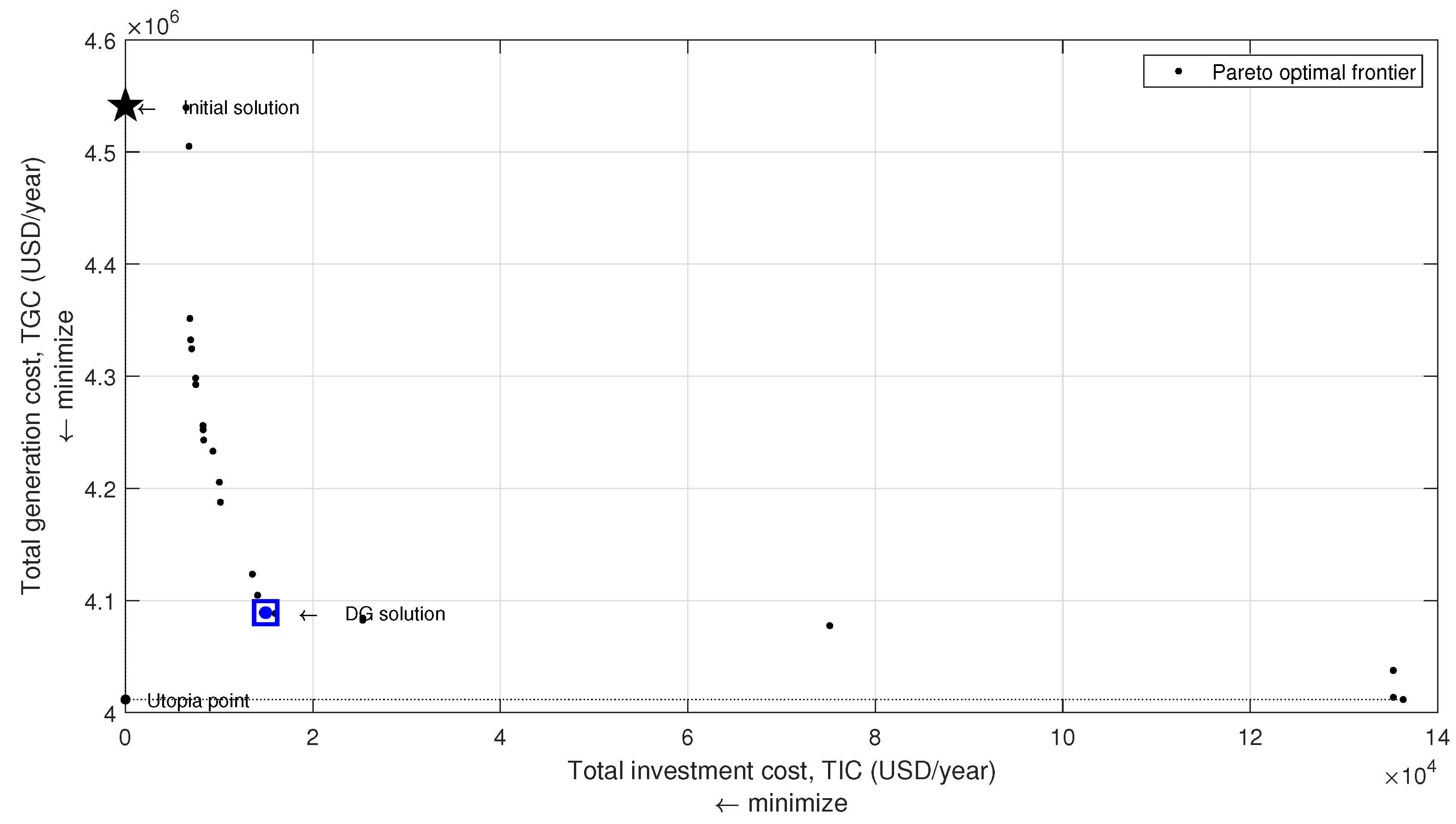
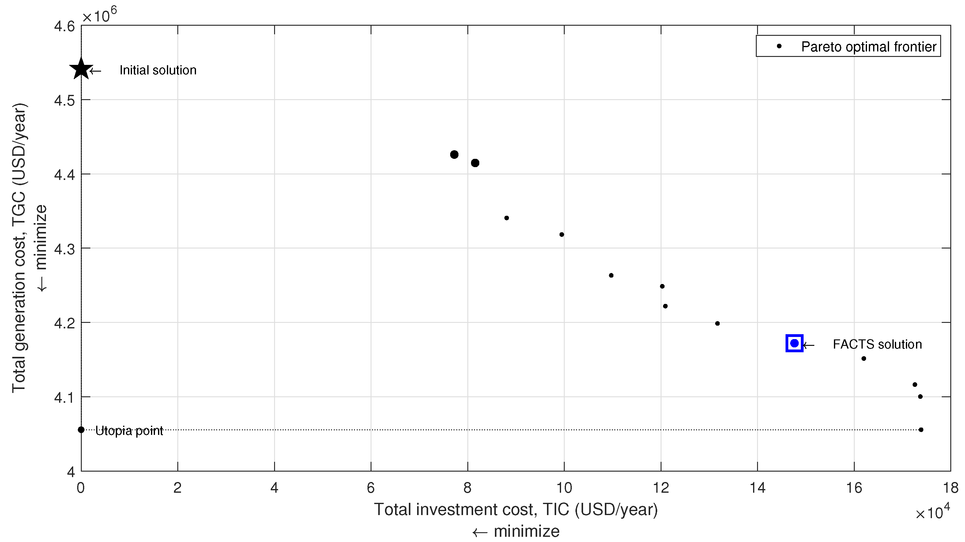
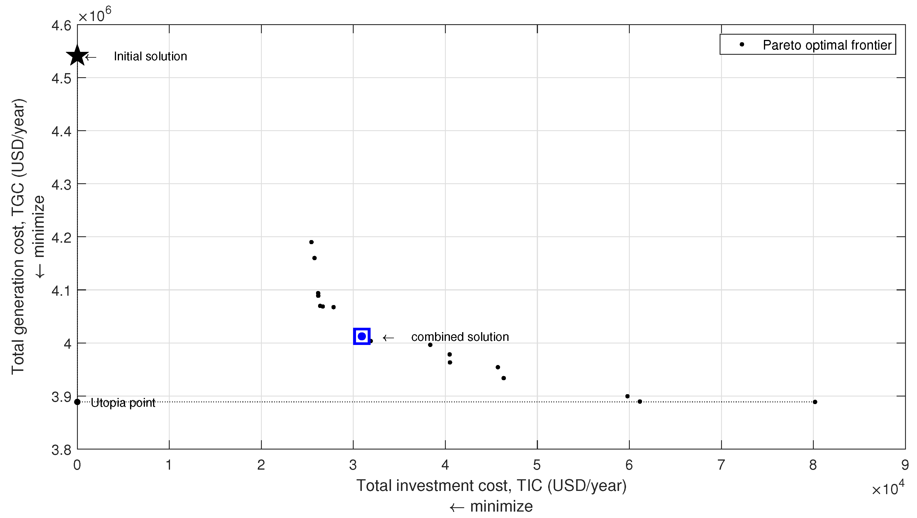
Three strategies were tested with the MOTS algorithm to improve the original case: the first strategy consists of adding only DG units, the second is to add only FACTS, and the third is a combined strategy that allows adding both DG units and FACTS. The comparison between these three strategies is analysed in this study by means of the Pareto optimal frontier, as shown in Figure 1, Figure 2 and Figure 3. The algorithm minimises two objectives: $TIC$ and $TGC$. “Black dots” are the solutions that are part of the Pareto front and the “star dot” is the initial solution. The range of variation of the $TGC$ is similar, but not equal, for the three strategies, however there are significant differences when the $TIC$ is compared. The DG installation is the cheapest strategy and the FACTS installation is the most expensive, while the combined strategy has intermediate costs.

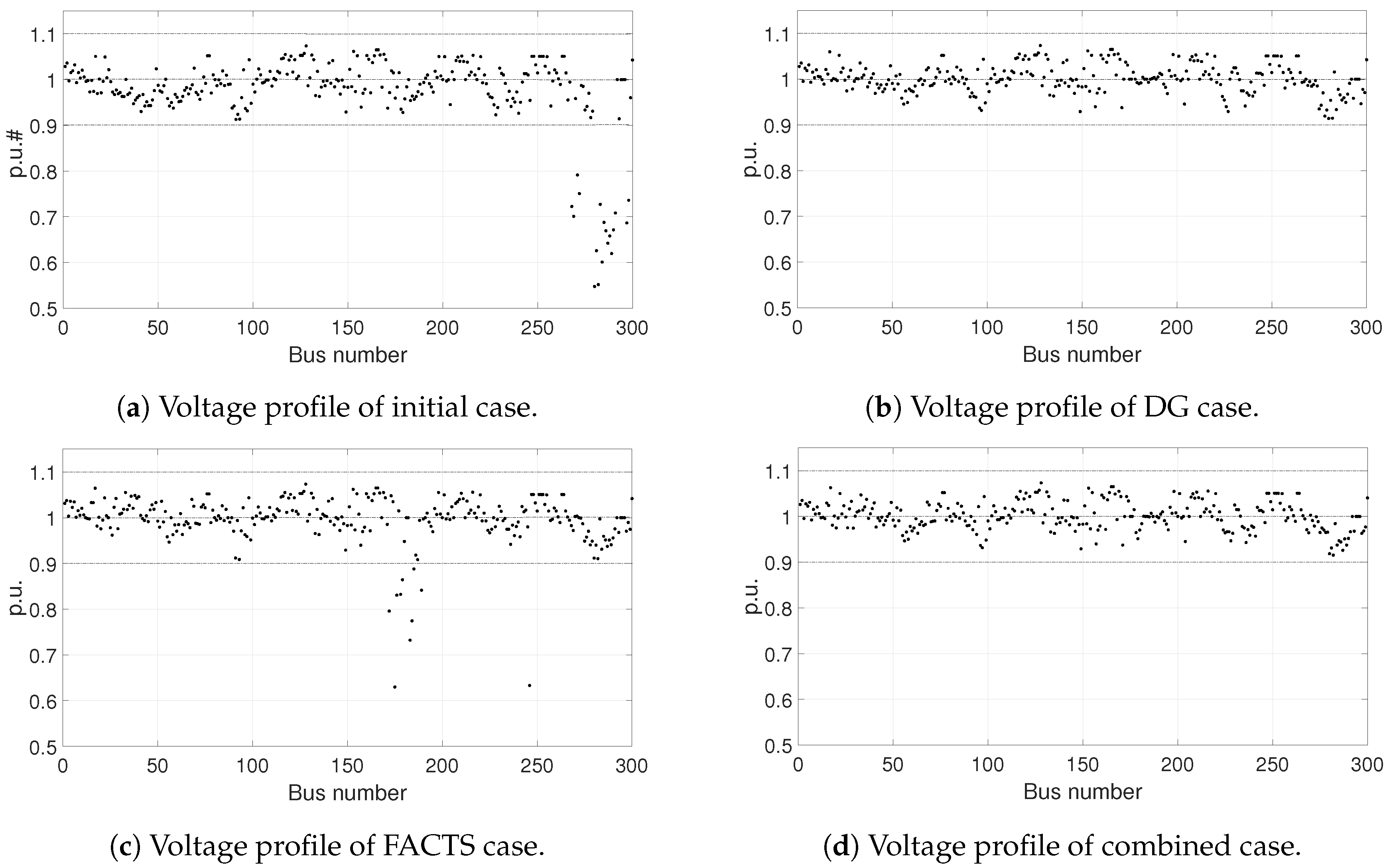
First, considering the Pareto front for the DG units case in Figure 1, it can be seen that the generation costs are low with relatively small investments, in the range of 0 to $2\times {10}^4$ USD/year. However, from that point on, strong investments, about $14\times {10}^4$ USD/year, are needed to only slightly reduce the cost of generation. In other words, the installation of DG is cheap, and reduces losses in the network, but eventually the network is saturated. Furthermore, in the DG units case, it is possible to keep the voltages within the allowed limits, as can be seen in Figure 4b. In the FACTS devices case, as shown in Figure 4c, it is possible to obtain generation costs similar to those obtained in the DG units case, although higher investments are necessary. In this case, there is also the disadvantage that it is not possible to maintain the voltages at all buses within their limits, as shown in Figure 4c; i.e., the voltage profile is improved, but not enough at all buses. Finally, in the Pareto front for the Combined devices case in Figure 3, it can be observed that the cost of generation may be reduced to a point below the minimum obtained in the previously mentioned cases. The solution for this case requires greater investments than in the DG units case, but much smaller than in the FACTS devices case, in the range of $2\times {10}^4$ to $8\times {10}^4$ USD/year. That is, the joint installation of DG and FACTS allows to solve the problems that a high penetration of DG in the network produces, decreasing the losses in the network and keeping the voltage profile within the permissible limits, as presented in Figure 4d.

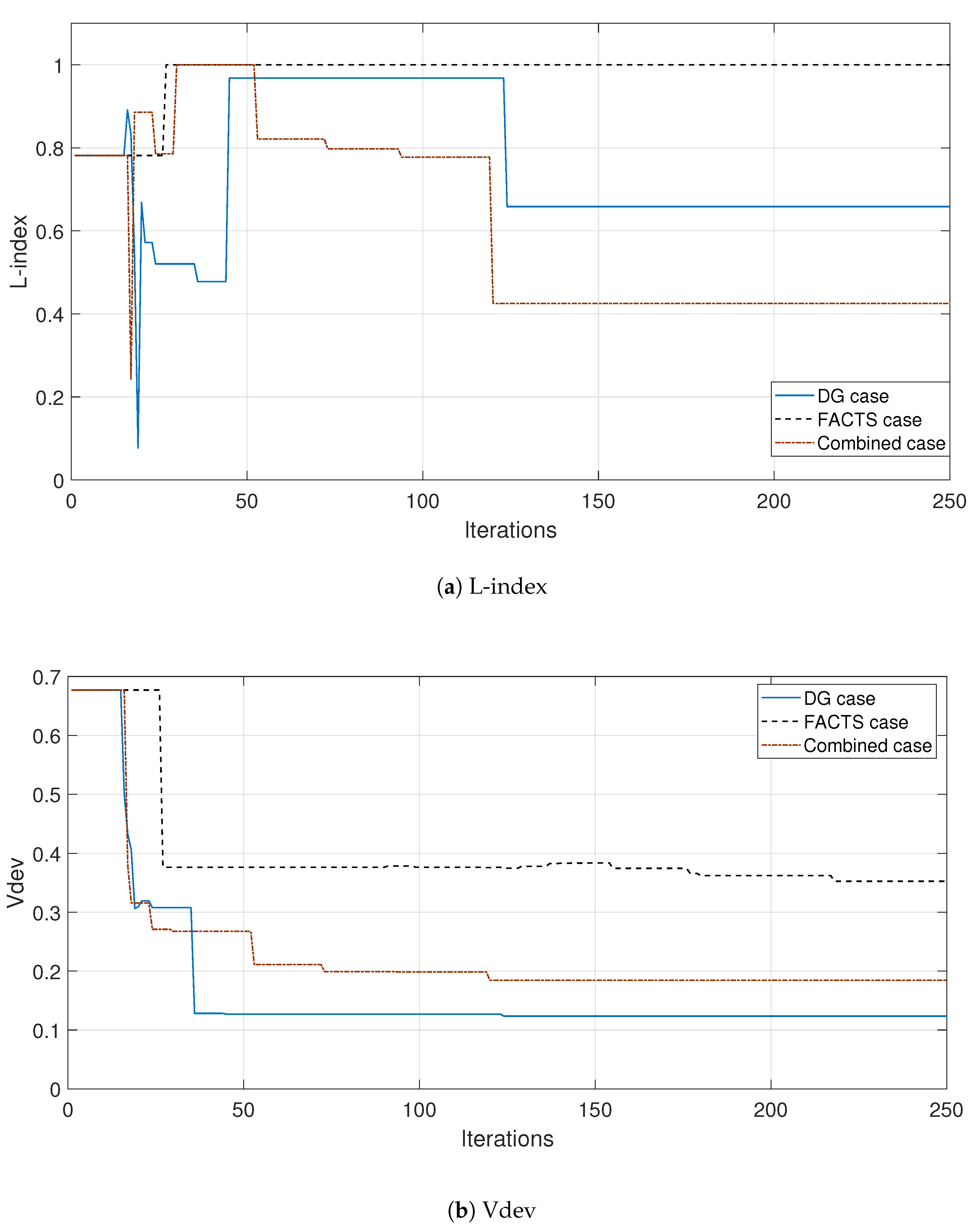
The algorithm monitors two technical indices during the search, shown in Figure 5, to determine if the technical characteristics of the solutions found with the different strategies are similar. These indices are: the L-index [82], which is a parameter that indicates the proximity of the node to voltage collapse, and the other is the difference between the reference voltage and the real voltage.

The L-index for add-only DG or add-only FACTS strategies approaches one, meaning that such solutions are near to the point of collapse. In contrast, for the combined strategy, a value further from the point of collapse is obtained. Thus, the inclusion of both DG and FACTS allows for the system to approach the limit operation point without collapse problems.

All the solutions of the Pareto curve are non-dominated, so to choose one, one must use an external criteria for the optimization to be carried out. The solution for each curve is the one with the best L-index and smallest voltage variation. These solutions are marked with a blue square in the Pareto curves and the description of location and characteristics of the installed devices are detailed in

Table 3. Location and characteristics of installed devices.

Stragtegy	Dev.	N	Observ.	Dev.	N	Observ.	Dev.	N	Observ.
Only DG	G	268	Cap = 1	G	190	Cap = 2	G	179	Cap = 1
	G	183	Cap = 8	G	93	Cap = 2	G	180	Cap = 1.2
	G	168	Cap = 2.5	G	175	Cap = 8	G	204	Cap = 1
	G	246	Cap = 1
Only FACTS	SVC	24	$\alpha =-0.6191$$v_m=0.99986$	SVC	81	$b=1.5$	SVC	266	$\alpha =-0.61726$$v_m=1.0014$
	SVC	87	$\alpha =-0.4941$$v_m=0.99992$	SVC	54	$b=-0.30335$	SVC	272	$\alpha =0.33423$$v_m=1.0001$
	SVC	38	$b=1.5$	SVC	89	$\alpha =0.62832$$v_m=1$	SVC	97	$b=1.5$
	SVC	208	$b=-1$	SVC	7	$b=1.5$	SVC	58	$b=0.07184$
	SVC	12	$\alpha =-0.52826$$v_m=0.99999$	SVC	57	$\alpha =0.95074$$v_m=0.99996$	SVC	188	$b=-0.35074$
	SVC	182	$\alpha =-0.19191$$v_m=0.99969$	SVC	168	$\alpha =1.0107$$v_m=0.99997$	SVC	227	$\alpha =0.81705$$v_m=0.99987$
	TCSC	267	$x=0.03279$	SSSC	381	$v_{cs}=2.5534$	UPFC	16	$v_p=0$$v_q=0.00001$$i_q=0.80591$
DG-FACTS	G	172	Cap = 2	G	189	Cap = 2	G	116	Cap = 1
	G	176	Cap = 8	G	184	Cap = 2	G	187	Cap = 0.8
	G	183	Cap = 1	G	175	Cap = 8	G	91	Cap = 1
	TCSC	13	$x=0.00323$	UPFC	179	$v_p=0$$v_q=0.02027$$i_q=-1$

Dev.: device type; N: bus or line location; Observ.: characteristics of device; $\alpha$: SVC firing angle; $v_m$: SVC measured voltage; b: SVC susceptance; x: TCSC series reactance; $v_{cs}$: SSSC voltage in quadrature with the line current; $v_p$: UPFC series voltage in phase with the line current; $v_q$: UPFC series voltage in quadrature with the line current; $i_q$: UPFC shunt current wich is in quadrature with the bus voltage in the line.

.

The $TIC$ plus the $TGC$ for the three strategies (DG, FACTS and combination) are presented in

Table 4. Costs results for selected solutions in [USD/year].

Description	Initial Solution	Only DG	Only FACTS	Combined Devices
$TIC$	0.00	14,958.00	147,639.31	30,924.21
$TGC$	4,541,173.09	4,089,150.61	4,172,071.38	4,012,460.96
Total cost	4,541,173.09	4,104,108.61	4,319,710.69	4,043,385.17
Save	–	−437,064.48	−221,462.40	−497,787.92

. The solution for only DG units has zero bus voltage violations and 38 lines are less saturated, obtaining a reduction of 437,064.48 USD/year compared to the initial solution. The solution with only FACTS devices obtains a 221,462.40 USD/year reduction in comparison with the initial solution, 47 lines are less saturated and the number of bus voltage violations is reduced to nine. The combination of DG and FACTS devices achieves a reduction of 497,787.92 USD/year in comparison to the initial solution, with zero bus voltage violations, and 53 lines less saturated.

Figure 4 depicts the bus voltage profiles comparison between the selected solutions for each strategy analysed in this work, where it can be seen that the first and third strategies provide better results. The second strategy (FACTS addition) is not able to reach an acceptable bus voltage profile improvement. The combination of DG and FACTS results in the best solution, finishing with more non-expenses and better bus voltage profile for all buses.

4. Conclusions

In this work, the capability of the proposed MOTS algorithm to find good solutions, in large-scale power systems, is demonstrated. By means of DG units implementation in the power system network, the bus voltage profile is improved, reaching zero violations. On the other hand, the add-only FACTS strategy is not able to reach zero bus voltage violations. Finally, the combination strategy with the installation of FACTS and DG units into the power system delivers better results than the other strategies analysed in this work. An excessive use of only FACTS devices or only DG units does not guarantee to enhance the power system stability nor to achieve power losses cost minimization; meanwhile, the combination of them reduces the total investment with improved expenses reduction. These conclusions are confirmed in the results presented in Table 4. The investment necessary to reach the solution of the DG units case is the lowest of the three cases, and an important amount of savings is obtained. However, it is not the best solution, because the solution of the Combined devices case, with only double the investment, allows to further decrease the generation cost and therefore amortize the investment, obtaining slightly higher savings than the DG units case. The FACTS devices case generates savings, but considerably less so than the other options. Maybe it could also be emphasized that with DG units alone, the saturation point is very close to the proposed solution, so that any generation cost improvement will require large investment costs, while the combined case allows for the reduction in generation cost to be more proportional to the investment cost.

These results are in line with the conclusions obtained in other papers. Singh’s review of DG impact in power systems [83] indicates that installing DG improves the voltage profile and reduces losses, among other benefits, but also warns that high DG penetration causes network problems. The authors of [84] comment that DG is advantageous over FACTS to improve the voltage profile. And in the papers [10,85], the advantages of the joint installation of DG and FACTS are discussed.

Below the most important practical information that can be extracted from this paper is summarized:

• DG installation is the cheapest measure that can be used in unsaturated networks, both to improve the voltage profile and to reduce losses.
• The installation of FACTS improves the network, but at higher prices.
• When the network is saturated with DG, it is also necessary to use FACTS to improve the network in terms of losses, voltages or even to improve stability.
• Locating multiple DG and FACTS units in a network is a complex problem that needs the help of specialized algorithms.

References

1. Song, Y.H.; Johns, A.T. Flexible AC Transmission Systems (FACTS); Institution of Engineering and Technology: London, UK, 1999. [Google Scholar]
2. Borbely, A.M.; Kreider, J.F. Distributed Generation: The Power Paradigm for the New Millennium; Mechanical and Aerospace Engineering Series; CRC Press: Boca Raton, FL, USA, 2001. [Google Scholar]
3. Acha, E.; Fuerte-Esquivel, C.R.; Ambriz-Pérez, H.; Angeles-Camacho, C. FACTS: Modelling and Simulation in Power Networks; John Wiley & Sons, Ltd.: Hoboken, NJ, USA, 2004. [Google Scholar] [CrossRef]
4. Vijayakumar, K.; Kumudinidevi, R.P. A new method for locating TCSC for congestion management in deregulated electricity markets. Int. J. Power Energy Convers. 2009, 1, 313–326. [Google Scholar] [CrossRef]
5. Pepermans, G.; Driesen, J.; Haeseldonckx, D.; Belmans, R.; D’haeseleer, W. Distributed generation: Definition, benefits and issues. Energy Policy 2005, 33, 787–798. [Google Scholar] [CrossRef]
6. Smallwood, C. Distributed generation in autonomous and nonautonomous micro grids. In Proceedings of the 2002 Rural Electric Power Conference. Papers Presented at the 46th Annual Conference (Cat. No. 02CH37360), Colorado Springs, CO, USA, 5–7 May 2002. [Google Scholar]
7. Hatziargyriou, N.; Meliopoulos, A. Distributed energy sources: Technical challenges. In Proceedings of the 2002 IEEE Power Engineering Society Winter Meeting. Conference Proceedings (Cat. No.02CH37309), New York, NY, USA, 27–31 January 2002. [Google Scholar]
8. Lasseter, R.; Piagi, P. Microgrid: A conceptual solution. In Proceedings of the 2004 IEEE 35th Annual Power Electronics Specialists Conference (IEEE Cat. No.04CH37551), Aachen, Germany, 20–25 June 2004. [Google Scholar]
9. Tian, W.; Zhang, Y.; Fu, R.; Zhao, Y.; Wang, G.; Winter, R. Modeling and Control Architecture of Source and Load Management in Islanded Power Systems. In Proceedings of the 2015 IEEE Energy Conversion Congress and Exposition (ECCE), Montreal, QC, Canada, 20–24 September 2015. [Google Scholar]
10. Singh, B.; Mukherjee, V.; Tiwari, P. A survey on impact assessment of DG and FACTS controllers in power systems. Renew. Sustain. Energy Rev. 2015, 42, 846–882. [Google Scholar] [CrossRef]
11. Zhang, X.P.; Rehtanz, C.; Pal, B. Flexible AC Transmission Systems: Modelling and Control (Power Systems); Springer: Berlin, Germany, 2006. [Google Scholar]
12. Padiyar, K.R. FACTS Controllers in Power Transmission and Distribution; New Age International (P) Limited.: Delhi, India, 2007. [Google Scholar]
13. Devaraj, D.; Roselyn, P. On-line voltage stability assessment using radial basis function network model with reduced input features. Int. J. Electr. Power Energy Syst. 2011, 33, 1550–1555. [Google Scholar] [CrossRef]
14. Tomin, N.; Zhukov, A.; Kurbatsky, V.; Sidorov, D.; Negnevitsky, M. Development of automatic intelligent system for on-line voltage security control of power systems. In Proceedings of the 2017 IEEE Manchester PowerTech, Manchester, UK, 18–22 June 2017. [Google Scholar] [CrossRef]
15. Satheesh, A. Maintaining power system stability with FACTS controller using bees algorithm and NN. J. Theor. Appl. Inf. Technol. 2013, 49, 38–47. [Google Scholar]
16. Acharya, N.; Sode-Yome, A.; Nadarajah, M. Facts about flexible AC transmission systems (FACTS) controllers: Practical installations and benefits. In Proceedings of the Australian Universities Power Engineering Conference (AUPEC), Melbourne, Australia, 25–28 September 2005; Volume 2, p. 6. [Google Scholar]
17. Nagesh, H.B.; Puttaswamy, P.S. Enhancement of voltage stability margin using FACTS controllers. Int. J. Comput. Electr. Eng. 2013, 5, 261–265. [Google Scholar] [CrossRef]
18. Habur, K.; O’Leary, D. FACTS for Cost Effective and Reliable Transmission of Electrical Energy Siemens-World Bank document–Final Draft Report, Erlangen. 2004. Available online: https://sites.google.com/site/lawking/facts_siemens.pdf (accessed on 20 February 2020).
19. Rashed, G.I.; Shaheen, H.I.; Cheng, S.J. Optimal location and parameter settings of multiple TCSCs for increasing power system loadability based on GA and PSO techniques. In Proceedings of the Third International Conference on Natural Computation (ICNC 2007), Haikou, China, 24–27 August 2007; Volume 1, pp. 1–10. [Google Scholar] [CrossRef]
20. Saravanan, M.; Slochanal, S.M.R.; Venkatesh, P.; Abraham, J.P.S. Application of PSO technique for optimal location of FACTS devices considering cost of installation and system loadability. Electr. Power Syst. Res. 2007, 77, 276–283. [Google Scholar] [CrossRef]
21. El Metwally, M.M.; El Emary, A.A.; El Bendary, F.M.; Mosaad, M.I. Optimal allocation of FACTS devices in power system using genetic algorithms. In Proceedings of the 2008 12th International Middle-East Power System Conference, Aswan, Egypt, 12–15 March 2008; pp. 1–4. [Google Scholar] [CrossRef]
22. Idris, R.M.; Khairuddin, A.; Mustafa, M.W. A multi-objective Bees Algorithm for optimum allocation of FACTS devices for restructured power system. In Proceedings of the TENCON 2009 IEEE Region 10 Conference, Singapore, 23–26 January 2009; pp. 1–6. [Google Scholar] [CrossRef]
23. Peikherfeh, M.; Abapour, M.; Moghaddam, M.P.; Namdari, A. Optimal allocation of FACTS devices for provision of voltage control ancillary services. In Proceedings of the 2010 7th International Conference on the European Energy Market, Madrid, Spain, 23–25 June 2010; Volume 23, pp. 1–5. [Google Scholar] [CrossRef]
24. Ara, A.L.; Kazemi, A.; Niaki, S.A.N. Multiobjective Optimal Location of FACTS Shunt-Series Controllers for Power System Operation Planning. IEEE Trans. Power Del. 2012, 27, 481–490. [Google Scholar] [CrossRef]
25. Deb, T.; Siddiqui, A.S. Congestion management through optimal placement of SSSC using modified gravitational search algorithm. Am. Int. J. Res. Sci. Technol. Eng. Math. (AIJRSTEM) 2017, 17, 66–69. [Google Scholar]
26. Pisica, I.; Bulac, C.; Toma, L.; Eremia, M. Optimal SVC placement in electric power systems using a genetic algorithms based method. In Proceedings of the 2009 IEEE Bucharest PowerTech, Bucharest, Romania, 28 June–2 July 2009; pp. 1–6. [Google Scholar] [CrossRef]
27. Chang, Y.C. Multi-objective optimal SVC installation for power system loading margin improvement. IEEE Trans. Power Syst. 2012, 27, 984–992. [Google Scholar] [CrossRef]
28. Taher, S.A.; Afsari, S.A. Optimal location and sizing of DSTATCOM in distribution systems by immune algorithm. Int. J. Electr. Power Energy Syst. 2014, 60, 34–44. [Google Scholar] [CrossRef]
29. Baghaee, H.R.; Kaviani, A.; Mirsalim, M.; Gharehpetian, B.G. Short circuit level and loss reduction by allocating TCSC and UPFC using particle swarm optimization. In Proceedings of the 2011 19th Iranian Conference on Electrical Engineering, Tehran, Iran, 17–19 May 2011; pp. 1–6. [Google Scholar]
30. Basu, M. Optimal power flow with FACTS devices using differential evolution. Int. J. Electr. Power Energy Syst. 2008, 30, 150–156. [Google Scholar] [CrossRef]
31. Singh, R.P.; Mukherjee, V.; Ghoshal, S.P. Particle swarm optimization with an aging leader and challengers algorithm for optimal power flow problem with FACTS devices. Int. J. Electr. Power Energy Syst. 2015, 64, 1185–1196. [Google Scholar] [CrossRef]
32. Mukherjee, A.; Mukherjee, V. Solution of optimal power flow with FACTS devices using a novel oppositional krill herd algorithm. Int. J. Electr. Power Energy Syst. 2016, 78, 700–714. [Google Scholar] [CrossRef]
33. John Grainger, W.S.J. Power System Analysis; McGraw-Hill series in electrical and computer engineering: Power and energy; McGraw-Hill: New York, NY, USA, 1994. [Google Scholar]
34. Weedy, B.M.; Cory, B.J.; Jenkins, N.; Ekanayake, J.B.; Strbac, G. Electric Power Systems; John Wiley and Sons Ltd.: West Sussex, UK, 2012. [Google Scholar]
35. Yorino, N.; El-Araby, E.E.; Sasaki, H.; Harada, S. A new formulation for FACTS allocation for security enhancement against voltage collapse. IEEE Trans. Power Syst. 2003, 18, 3–10. [Google Scholar] [CrossRef]
36. Cai, L.J.; Erlich, I.; Stamtsis, G. Optimal choice and allocation of FACTS devices in deregulated electricity market using genetic algorithms. In Proceedings of the IEEE PES Power Systems Conference and Exposition, New York, NY, USA, 10–13 October 2004; pp. 201–207. [Google Scholar] [CrossRef]
37. Gitizadeh, M.; Kalantar, M. A new approach for congestion management via optimal location of FACTS devices in deregulated power systems. In Proceedings of the Third International Conference on Electric Utility Deregulation and Restructuring and Power Technologies, Nanjing, China, 6–9 April 2008; pp. 1592–1597. [Google Scholar] [CrossRef]
38. Gitizadeh, M.; Kalantar, M. Genetic algorithm based fuzzy multi-objective approach to FACTS devices allocation in FARS regional electric network. Int. J. Sci. Technol. 2008, 15, 534–546. [Google Scholar]
39. Gitizadeh, M. Allocation of multi-type FACTS devices using multi-objective genetic algorithm approach for power system reinforcement. Electr. Eng. 2010, 92, 227–237. [Google Scholar] [CrossRef]
40. Benabid, R.; Boudour, M.; Abido, M.A. Optimal location and setting of SVC and TCSC devices using non-dominated sorting particle swarm optimization. Electr. Power Syst. Res. 2009, 79, 1668–1677. [Google Scholar] [CrossRef]
41. Benabid, R.; Boudour, M.; Abido, M.A. Optimal placement of FACTS devices for multi-objective voltage stability problem. In Proceedings of the IEEE/PES Power Systems Conference and Exposition, Seattle, WA, USA, 15–18 March 2009. [Google Scholar] [CrossRef]
42. Wibowo, R.S.; Yorino, N.; Eghbal, M.; Zoka, Y.; Sasaki, Y. FACTS devices allocation with control coordination considering congestion relief and voltage stability. IEEE Trans. Power Syst. 2011, 26, 2302–2310. [Google Scholar] [CrossRef]
43. Laïfa, A.; Medoued, A. Optimal FACTS location to enhance voltage stability using multi-objective harmony search. In Proceedings of the 3rd International Conference on Electric Power and Energy Conversion Systems, Istanbul, Turkey, 2–4 October 2013; Volume 1, p. 6. [Google Scholar] [CrossRef]
44. Bhattacharyya, B.; Kumar, S. Reactive power planning with FACTS devices using gravitational search algorithm. Ain Shams Eng. J. 2015, 6, 865–871. [Google Scholar] [CrossRef] [Green Version]
45. Mohammadi, M.; Rezazadeh, A.; Sedighizadeh, M. Optimal placement and sizing of FACTS devices for loadability enhancement in deregulated power systems. Recent Re. Artif. Intell. Database Manag. 2019, 12, 148–156. [Google Scholar]
46. Sugimoto, J.; Yokoyama, R.; Niimura, T.; Fukuyama, Y. Tabu search based-optimal allocation of voltage control devices by connections ofdistributed generators in distribution systems. In Proceedings of the 39th International Universities Power Engineering Conference, UPEC 2004, Bristol, UK, 6–8 September 2004. [Google Scholar]
47. Bhasaputra, P.; Ongsakul, W. Optimal placement of multi-type FACTS devices by hybrid TS/SA approach. In Proceedings of the 2003 International Symposium on Circuits and Systems, 2003. ISCAS ’03, Bangkok, Thailand, 25–28 May 2003. [Google Scholar]
48. Chansareewittaya, S.; Jirapong, P. Total transfer capability enhancement with optimal number of FACTS controllers using hybrid TSSA. In Proceedings of the IEEE Southeastcon, Orlando, FL, USA, 15–18 March 2012. [Google Scholar]
49. Mori, H.; Tani, H. Two-staged tabu search for determining optimal allocation of D-FACTS in radial distribution systems with distributed generation. In Proceedings of the IEEE/PES Transmission and Distribution Conference and Exhibition, Yokohama, Japan, 6–10 October 2002. [Google Scholar]
50. Ebrahimi, S.; Farsangi, M.; Nezamabadi-Pour, H.; Lee, K. Optimal allocation of static VAr compensators using modal analysis, simulatedannealing and tabu search. In Proceedings of the IFAC Proceedings Volumes, Kananaskis, AB, Canada, 25–28 June 2006. [Google Scholar]
51. Maciel, R.; Padilha-Feltrin, A. Distributed Generation Impact Evaluation Using a Multi-Objective Tabu Search. In Proceedings of the 2009 15th International Conference on Intelligent System Applications to Power Systems, Curitiba, Brazil, 8–12 November 2009. [Google Scholar]
52. Milano, F. An Open Source Power System Analysis Toolbox. Trans. Power Syst. 2005, 20, 1199–1206. [Google Scholar] [CrossRef]
53. Glover, F.W.; Laguna, M. Tabu Search; Number 1 in Tabu Search; Springer: Berlin, Germany, 1998. [Google Scholar] [CrossRef]
54. Pereira, B.R.; Cossi, A.M.; Contreras, J.; Mantovani, J.R.S. Multiobjective multistage distribution system planning using tabu search. IET Gener. Transm. Distrib. 2013, 8, 35–45. [Google Scholar] [CrossRef] [Green Version]
55. Singh, S.N.; David, A.K. Placement of FACTS devices in open power market. In Proceedings of the APSCOM 2000—5th International Conference on Advances in Power System Control, Operation and Management. Institution of Engineering and Technology, Hong Kong, China, 30 October–1 November 2000; pp. 173–177. [Google Scholar] [CrossRef]
56. Singh, S.N.; David, A.K. A new approach for placement of FACTS devices in open power markets. IEEE Power Eng. Rev. 2001, 21, 58–60. [Google Scholar] [CrossRef]
57. Ippolito, L.; Siano, P. Selection of optimal number and location of thyristor-controlled phase shifters using genetic based algorithms. IEE Proc.-Gener. Transm. Distrib. 2004, 151, 630–637. [Google Scholar] [CrossRef]
58. Ippolito, L. A novel strategy for selection of the optimal number and location of UPFC devices in deregulated electric power systems. In Proceedings of the 2005 IEEE Russia Power Tech, St. Petersburg, Russia, 27–30 June 2005; pp. 1–9. [Google Scholar] [CrossRef]
59. Ippolito, L.; Cortiglia, A.L.; Petrocelli, M. Optimal allocation of FACTS devices by using multi-objective optimal power flow and genetic algorithms. Int. J. Emerg. Electr. Power Syst. 2006, 7. [Google Scholar] [CrossRef]
60. Eghbal, M.; Yorino, N.; Zoka, Y. Comparative study on the application of modern heuristic techniques to SVC placement problem. J. Comput. 2009, 4. [Google Scholar] [CrossRef]
61. Joorabian, M.; Saniei, M.; Sepahvand, H. Locating and parameters setting of TCSC for congestion management in deregulated electricity market. In Proceedings of the 6th IEEE Conference on Industrial Electronics and Applications, Beijing, China, 21–23 June 2011; Volume 1, pp. 2185–2190. [Google Scholar] [CrossRef]
62. Taher, S.A.; Amooshahi, M.K. New approach for optimal UPFC placement using hybrid immune algorithm in electric power systems. Int. J. Electr. Power Energy Syst. 2012, 43, 899–909. [Google Scholar] [CrossRef]
63. Iqbal, F.; Khan, M.T.; Siddiqui, A.S. Optimal placement of DG and DSTATCOM for loss reduction and voltage profile improvement. Alex. Eng. J. 2017, 57, 755–765. [Google Scholar] [CrossRef]
64. Hartel, P.; Vrana, T.K.; Hennig, T.; von Bonin, M.; Wiggelinkhuizen, E.J.; Nieuwenhout, F.D.J. Review of investment model cost parameters for VSC HVDC transmission infrastructure. Electr. Power Syst. Res. 2017, 151, 419–431. [Google Scholar] [CrossRef] [Green Version]
65. Alabduljabbar, A.A.; Milanovic, J.V. Genetic algorithm based optimization for allocation of static VAr compensators. In Proceedings of the 8th IEE International Conference on AC and DC Power Transmission (ACDC 2006), London, UK, 28–31 March 2006; Volume 1, pp. 115–119. [Google Scholar] [CrossRef]
66. Chandrasekaran, K.; Jeyaraj, K.A.; Sahayasenthamil, L.; Saravanan, M. A new method to incorporate FACTS devices in optimal power flow using particle swarm optimization. J. Theor. Appl. Inf. Technol. 2009, 5, 67–74. [Google Scholar]
67. Nabavi, S.M.; Hajforoosh, S.; Hajforoosh, S.; Karimi, A.; Khafafi, K. Maximizing the overall satisfaction degree of all participants in the market using real code-based genetic algorithm by optimally locating and sizing the thyristor-controlled series capacitor. J. Electr. Eng. Technol. 2011, 6, 493–504. [Google Scholar] [CrossRef] [Green Version]
68. Zhong, J.; Bhattacharya, K. Toward a competitive market for reactive power. IEEE Trans. Power Syst. 2002, 17, 1206–1215. [Google Scholar] [CrossRef]
69. An, S.; Condren, J.; Gedra, T.W. An ideal transformer UPFC model, OPF first-order sensitivities, and application to screening for optimal UPFC locations. IEEE Trans. Power Syst. 2007, 22, 68–75. [Google Scholar] [CrossRef]
70. Blanco, G.; Olsina, F.; Garces, F.; Rehtanz, C. Real option valuation of FACTS investments based on the least square Monte Carlo method. IEEE Trans. Power Syst. 2011, 26, 1389–1398. [Google Scholar] [CrossRef]
71. Niknam, T.; Narimani, M.; Aghaei, J.; Azizipanah-Abarghooee, R. Improved particle swarm optimisation for multi-objective optimal power flow considering the cost, loss, emission and voltage stability index. IET Gener. Transm. Distrib. 2012, 6, 515. [Google Scholar] [CrossRef]
72. Tlijani, K.; Guesmi, T.; Abdallah, H.H.; Ouali, A. 0ptimal location and parameter setting of TCSC based on sensitivity analysis. In Proceedings of the 2012 First International Conference on Renewable Energies and Vehicular Technology, Hammamet, Tunisia, 26–28 March 2012; Volume 1, pp. 420–424. [Google Scholar] [CrossRef]
73. INEGI. Economic Information Bank. 2020. Available online: https://www.inegi.org.mx/sistemas/bie/ (accessed on 20 February 2020).
74. Chen, L.; Zhong, J.; Gan, D. Reactive power planning and its cost allocation for distribution systems with distributed generation. In Proceedings of the 2006 IEEE Power Engineering Society General Meeting, Montreal, QC, Canada, 18–22 June 2006; p. 6. [Google Scholar] [CrossRef] [Green Version]
75. CFE. Price per Requested Work. 2020. Available online: https://app.cfe.mx/Aplicaciones/OTROS/Aportaciones/MenuAportaciones.aspx (accessed on 20 February 2020).
76. Milano, F. Power System Modelling and Scripting; Power Systems; Springer: Berlin/Heidelberg, Germany, 2010. [Google Scholar] [CrossRef]
77. Milano, F. Power system analysis toolbox (PSAT). Available online: http://faraday1.ucd.ie/psat.html (accessed on 6 March 2019).
78. Matlab. Matlab Documentation; Mathworks: Natick, MA, USA, 2017. [Google Scholar]
79. Papachristoudis, G. Kruskal Algorithm. Mathworks File Exchange. 2014. Available online: https://la.mathworks.com/matlabcentral/fileexchange/41963-kruskal-s-algorithm (accessed on 20 February 2020).
80. Arcia-Garibaldi, G.; Cruz-Romero, P.; Gómez-Expósito, A. Future power transmission: Visions, technologies and challenges. Renew. Sustain. Energy Rev. 2018, 94, 285–301. [Google Scholar] [CrossRef]
81. University of Washington. Power Systems Tests Case Archive. 2020. Available online: https://labs.ece.uw.edu/pstca/pf300/pg_tca300bus.htm (accessed on 20 February 2020).
82. Kessel, P.; Glavitsch, H. Estimating the voltage stability of a power system. IEEE Trans. Power Del. 1986, 1, 346–354. [Google Scholar] [CrossRef]
83. Singh, B.; Sharma, J. A review on distributed generation planning. Renew. Sustain. Energy Rev. 2017, 76, 529–544. [Google Scholar] [CrossRef]
84. Chatterjee, S.; Nath, P.; Biswas, R.; Das, M. Advantage of DG for improving voltage profile over facts devices. Int. J. Eng. Res. Appl. 2013, 3, 2029–2032. [Google Scholar]
85. Bharathi Dasan, S.; Gayatri, S.; Lavanya, V.; Praveena, N.; Preethi, T. FACTS based voltage enhancement in hybrid DG distribution system with mixed load model. J. Electr. Eng. 2012, 12, 188–196. [Google Scholar]
Figure 1. Pareto optimal frontier for the DG units case.
Energies 13 02722 g001
Figure 2. Pareto optimal frontier for the FACTS devices case.
Energies 13 02722 g002
Figure 3. Pareto optimal frontier for the combined units case.
Energies 13 02722 g003
Figure 4. Bus voltage profile for the selected solutions on each strategy.
Energies 13 02722 g004
Figure 5. Evolution of technical parameters in the MOTS search.
Energies 13 02722 g005