Abstract
This paper presents a new linear state estimation model based on a current summation load flow method for three-phase distribution systems. The developed estimator may be applied to both the supervision of distribution systems under normal operating conditions and the fault location in cases of low and high impedance faults. Our studies were conducted using a real distribution feeder. For fault location analysis, the system was modeled using the ATP (alternative transient program) in order to emulate measurements of voltages and currents at the substation, and voltage magnitudes registered by other meters during the fault. We used the MATLAB™ software to process the algorithms. The main contributions that arose after integrating the current method into system supervision in case of network failures under normal operating conditions and the fault location are as follows: (i) estimation of system losses; (ii) modeling of loads in real time to consider their contributions in the fault location process; and (iii) low influence of fault resistance in the location algorithm. The results show that the proposed method has good precision, low computational processing time, and is promising for distribution system supervision with a reduced number of meters.
1. Introduction
Current energy systems have undergone intense modifications over the past few decades to provide the end-user with a reliable and quality electricity supply. With the exponential increase in consumers, generation diversification, and increase in power quality requirements, there was a need to improve the operation and planning structures within electric power systems. Traditionally, methods for both the load flow calculation and state estimation are used for these purposes and are the focus of several studies that examine electrical power systems.
The purpose of the load flow calculation and the state estimator is to determine voltages in magnitude and angle for all nodes of the grid, given a specific configuration and a load condition. From the known voltages, the active and reactive power flow in the branches and the active and reactive powers generated, consumed, and lost in the system are calculated. Although they present similar objectives, the load flow is used in both network operation and planning—i.e., in off-line applications—whereas state estimation is generally used in control and supervision centers and consist of an online application.
It is noteworthy that most state estimators described in the literature were developed based on the classical model for power transmission systems, while there are a smaller number of studies about estimators applied to distribution networks. In order to estimate the state of a power distribution system by applying traditional algorithms, it is necessary to obtain measured data in real time. However, most feeders usually have just one measurement set at the output of the substation, compromising system observability and making it inadequate for estimation. Thus, it is necessary to use pseudo-measurements [1,2]. Pseudo-measurements are values of quantities obtained from measurements of two or more other quantities, which contain errors [3]. As an example, the power pseudo-measures are built from current and voltage measures, whose uncertainties about the pseudo-measure value need to be determined. They can be constructed by means of indirect measurements (i.e., measurements of quantities that are related) through circuit equations, with the quantities to be measured. They can also be obtained from the information obtained offline, assuming greater errors are admitted than those inherent in measuring equipment. Information traditionally used for distribution system planning was adopted as pseudo-measures, such as transformers utilization factors. In these cases, a relatively high margin of error of ±20% was admitted in order to compute the corresponding variances.
The use of the state estimation method for fault location in distribution networks has been the focus of recent studies [4,5,6,7,8,9]. These techniques can be classified according to location, quantity, and technology of the available monitoring infrastructure [10]. The method proposed by Gord et al. [9] estimates the fault location based on a comparison between the stored current and voltages measured at the beginning of the feeder with the corresponding values obtained by simulating short circuits at different points of a distribution system. Moreover, the work determines the faulted section by calculating an index developed by analyzing the frequency components. Dashti and Sadeh [11] propose a method based on impedance using dynamic load estimation and a distributed parameter line model. As has been previously reported, dynamic load estimation contributes to increased accuracy in the region under fault. Moreover, Vieira et al. [12] presented a new method for detecting and locating high impedance faults (HIF) in primary networks using unbalanced voltage measurements collected from smart meters (SMs), which were installed in low voltage end customers. Li et al. [13] proposes a program for analyzing faults in distribution systems in association with pattern recognition methods, database searches, and phasors obtained from the feeder root node. A non-linear state estimator based on power summation was proposed by Almeida et al. [14]. In this work, the authors estimate only one phase of the system, using the single-phase equivalent to determine the state of the other phases.
This paper proposes a new multi-purpose linear state estimator based on the current summation method for real-time supervision of distribution networks under normal operating conditions and for fault location. During normal operation, the algorithm uses current and voltages measured in real time to estimate current pseudo-measures, through the use of utilization and load imbalance factors, which are constantly updated. In a second step, the estimator performs load estimation, bus voltages, branch currents, and total network losses for each time window defined by the network operator. In the event of a fault, the estimator initializes the localization mode by assuming that each bus in the system is short-circuited once, sequentially, replacing the currents of these loads with a value that results from the subtraction of the fault current measured in the substation minus the estimated load currents of the other nodes in the system. For each assumption, we estimate the voltages of the nodes and currents of all branches of the system. These estimated data are compared with the data acquired from the meters installed along the feeder, which makes it possible to define the fault location as having the least variation between the measured and estimated data. Objectively, this method uses a state estimator developed specifically to determine the state of distribution networks to locate faults in this type of system using real-time data, avoiding the use of state estimators made for transmission system analysis.
Simulations were performed to verify the robustness of the method on the various fault scenarios in distribution networks. These included: feeder location, fault type, influence of low and high faults impedance, and the influence of system load level and load modeling. The method was validated using a real distribution system located in northeastern Brazil, which was modeled in the ATP (alternative transient program), in order to obtain the phasors of short circuit simulations.
This article has the following structure: Section 2 presents a general approach to the state estimation theory; Section 3 demonstrates how adjustments are made to system loads by calculating load and load imbalance factors; Section 4 reviews the current summation method; Section 5 addresses the linear state estimation model proposed by this work, both for normal operating conditions and for the fault condition; Section 6 shows the computer simulation results for a real 58-node distribution system, simulated by the ATP and MATLAB™, which verified the behavior of the algorithm in the operating condition and addressed various conditions that can influence the location of faults, such as the resistance of fault, the type of fault, and the influence of the load level; in Section 7, numerical results are discussed; and lastly, in Section 8, conclusions are presented.
2. State Estimation
In most current power distribution networks, it is economically unviable to use measuring units in all branches of the feeder. However, it is of great importance for the system operator to have an approximate estimate of network conditions that are specified by variables like voltages and currents. In this case, the unmeasured variables must be estimated based on the measurement information present in the system [15]. Mathematically, the problem of state estimation is fundamentally constituted by an overdetermined system of non-linear equations [16]. The relationship between the measured (or pseudo-measured) values of the monitored quantities with the state variables is established in Equation (1):
where z is the vector of measurements (and pseudo-measurements) with dimension (m × 1). m is the total number of performed measurements and x is the vector of state variables. In dimension (n × 1), m > n (overdetermined system). h(x) is the vector of functions that relates state variables to measurements and pseudo-measurements and e is the error vector of the measurements and pseudo-measurements, with dimension (m × 1).
It is necessary to optimize Equation (2) according to the weighted least squares methodology, i.e., it is necessary to minimize the objective function J(x) [3]:
The weights are considered by means of the covariance matrix Rz. The estimated state variables are updated using iterative methods, usually Gauss–Newton or Newton–Raphson, according to Equations (3) and (4).
In Equations (3) and (4), t represents the iteration counter and g(x) and G(x) represent the gradient of J(x) and the gain matrix, respectively. According to the Newton–Raphson method, the Taylor expansion in Equation (1) is used, resulting in Equation (5).
Combining Equations (2) and (5) give:
where H(x) = ∂h/∂x represents the Jacobian matrix. Extracting the first-order term from J(x) gives:
That leads to:
In comparison to Equation (3), the gain matrix is:
It is important to emphasize that the solution of Equation (8) and the determination of G require a great computational effort. Moreover, the iterative process derives from a linearization of the nonlinear functions h(x). If the measurement model given by Equation (1) has only linear functions, then, according to Equation (8), the estimated vector, Δx, can be calculated directly by equation of the linearized state estimator, where x can be obtained through the explicit solution of the normal Gauss equation, as described in Equations (10) and (11).
3. Load Adjustment Process
In this work, an efficient load-adjustment algorithm for a three-phase distribution feeder is implemented in conjunction with a linear state estimator based on the current summation load flow method. Since the distribution feeders have a small number of measurement points, it is necessary to introduce pseudo-measurements in the measurement vector. However, the fact that most measurements used in state estimation are pseudo-measurements reveals the paramount importance of their appropriate modeling, so they shall represent the network conditions as realistic as possible [17]. Before the estimation process, the utilization factor, the factor of load imbalance and the power factor are used to define the loads [14,18]. These factors are commonly used in load flow algorithms to calculate the power injected at the nodes and are considered as fixed values, whereas in the state estimation algorithm the same factors are updated in the estimation process.
The utilization factor indicates the percentage of the installed load that is being used and frequently has a fixed value when applied to the load flow methods used for planning purposes. In this work, the calculation of the system utilization factor presents a distinct dynamic, being updated according to the variation of measured current and voltage data [18]. In addition, a utilization factor will be used for each point of the feeder that has real-time metering for each phase, so the following expression will be used:
In Equation (12):
: Utilization factor calculated for a measuring point i, where i indicates the number of measurement points of the system.
: Phase current measured in real time at measurement point i.
: Rated current of a distribution transformer, where j indicates the number of the transformer, up to the maximum number of transformers downstream of point i, defined by nt.
: Rated current of a transformer (Group A consumers), where k indicates the number of the transformer, up to the maximum number of private consumers downstream of point i, defined by ng.
Consider the measurement points 1 and 2 in Figure 1. Since the reduced system of Figure 1 has two measurement points, it becomes necessary to calculate two utilization factors fu1 and fu2 for meters 1 and 2. It is important to note that when calculating the utilization factor 1, all transformers downstream of the measurement point 1, with their respective powers, are considered in the calculation of fu1, whereas only the transformers downstream of the measurement point 2 are used to compute fu2. After calculating the utilization factor of each measurement point, the loads of each node must be linked to the corresponding measurement point and adjusted according its respective utilization factor. Based on Figure 1, the utilization factor fu1 should be applied in the adjustment of loads between measuring points 1 and 2, while the utilization factor fu2 should be applied downstream of measurement point 2. This procedure is repeated while several measurement points are present.
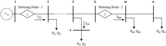
Figure 1.
Simplified representation of a primary distribution network.
The state estimator developed in this work evaluates the three phases of a distribution system to consider the inherent imbalanced characteristics of this type of electrical network. For this reason, in addition to the adjustments carried out using the utilization factor, it is necessary to define the imbalance of loads to be able to consider the imbalance in the calculation of the three-phase state estimator. Consider as the total power required by a given three-phase load of the system and is the rated power of the transformer connected to bus.
Assuming that the ratio between the power of a specific phase α and the current measured in this phase is equal to the ratio between the total power required by the load and the sum of measured currents of the three phases, as described in Equation (14), it is possible to obtain an estimate for the power of load per phase, according to Equation (15).
The term in parentheses of Equation (15) provides the relationship between a specific phase current magnitude in relation to the sum of all phases currents measured at a given point in the system. This relationship is called the load imbalance factor, shown in Equation (16). The power per phase of a three-phase load cane be summarized as Equations (17) [18].
As well as the utilization factor, the factor of load imbalance should only be applied to the loads belonging to the measurement zone of a given meter, although, for its calculation, uses the measured currents from the loads downstream of the measurement point. The calculated according to Equation (16) are applicable to distribution transformers. For private consumers and capacitor banks a factor of 1/3 must be applied, since in these cases the demands per phase are practically balanced.
The fact that the measured currents are used to determine the factor of load unbalance does not necessarily mean that the estimated voltages at nodes will be balanced, considering that in the Forward Sweep process, each phase will estimate the node voltages according to the previously pseudo-measured currents estimated, which will be unbalanced if the measured currents are unbalanced, according to Equation (16). If there is a voltage imbalance in the meters installed along the feeder, there will be no limitation of the algorithm in this regard, considering that the measured voltage data will always be taken as reference nodes in the reduction section under analysis, as shown in the Section 5.2.
4. Currents Summation Method
The currents summation method was initially developed by [19] and received several generalizations over the years [20,21,22,23]. Basically, the method uses the sum of branch currents to determine the power flow of the system. As in the powers summation method, the algorithm consists of two sweeps, from the final nodes to the substation and from the substation to the end nodes, called backward sweep and forward sweep, respectively.
The estimation is accomplished for each reduction section [18] after calculation of the currents accumulated for all branches of the system.
The current calculated for a generic node n in the measurement region of a meter k, , is obtained by Equation (18).
where α indicates the analyzed phase.
As loads are calculated, it is possible to determine the accumulated currents at each branch of the system in the backward sweep process. In the case of a l-m and m-n sections, the current of the branches, located upstream of the system is given by:
Subsequently, after sweeping the entire system, the forward sweep process is implemented along with the state estimator. In this step, the estimator calculates the new values of node voltages by using pseudo-measurements and the theory of uncertainty propagation (propagation of errors) to model their respective errors. Starting from the substation node, the downstream node voltages are calculated according to Equation (20), considering the nominal voltage at the substation node and the total current accumulated in the backward sweep step.
After the new node voltages are updated, the currents of each system load must be recalculated using Equation (18). The scan procedure is repeated until the voltage difference between two iterations is less than a specified tolerance.
When the convergence is reached, the losses of each branch can be determined from the estimated currents flowing through the reduction section. Since the line parameters of a given section m-n are constant, the losses may be calculated from Equations (21) and (22).
To calculate the total system losses, just add the losses of each branch of the feeder.
5. Linear Current Summation State Estimation
Since the currents at each node are defined, whether they are representing a distribution transformer or private consumer, the algorithm performs the estimation of voltages and currents for each system section, scanning the feeder from substation to the terminal nodes. These sections, named reduction sections (RS), are composed of at least two system nodes and can contain, as shown below, the following types of nodes:
- Reference node: It is the upstream node of the reduction section whose voltage and current values serve as reference for the estimation of voltage at node(s) downstream belonging to the same reduction section.
- Reduction node: Node that represents the rest of the system, accumulating all the power flow from the nodes downstream.
- Terminal node(s): Represents the end of a section, where the only current flowing is from load.
The results of the estimation for a RS are used as pseudo-measurement to estimate the subsequent section, so that the process is carried out until the currents and voltages of the whole feeder has been estimated.
For a better understanding about the variables involved in the construction of the model, consider that in Figure 2 Vn is the voltage at n-node, where n represents the analyzed node; Imn represents the branch current between two buses m and n; In is the current required by transformers located at node n; and Isum_n is assumed as being the current at reduced node n, which is calculated by the sum of all currents associated with the nodes downstream of n.
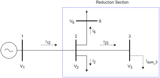
Figure 2.
Single line diagram of reduction section 1.
It is important to point out that the linearized state estimation based on current summation do not neglect the losses. After estimating the currents of the reduction sections, the losses are calculated using corresponding R and X parameters of each branch belonging to the section. In a simplified way, the method may be summarized in the following steps:
- Step 1: Read system file with corresponding data.
- Step 2: Select a phase to be analyzed.
- Step 3: Determine the factor of load imbalance (Equation (15)) and apply the utilization factor (Equation (12)).
- Step 4: Calculate the currents demanded of each node and the currents of the system branches.
- Step 5: Replace the pseudo-measured quantities of the nodes that contain measurement equipment by measured values.
- Step 6: Start the iterative state estimation process.
- Step 7: Construct the measurement model of the reduction section: x, z, h(x), H and R.
- Step 8: Assume pre-set or corrected values for the state variables.
- Step 9: Calculate Δz and obtain Δx(t) by the normal Gaussian equation (Equation (11)).
- Step 10: Determine
- If <tolerance
- Stop RS estimation and save results
- Or
- Actualize the state variables by the corrected values and return to step 8
- Step 11: If there is any RS to estimate
- Return to step 6
- Or
- Finish the iterative process, determine the load flows and the technical losses of the system and display results.
The steps above are performed for all phases. At the end of the entire process, total technical losses are added up and depicted in a report along with the currents, voltages and power flow estimated for each phase.
5.1. Re-Estimation Process
On the proposed algorithm, an iterative process of re-estimation of the states based on the system sweeping method was implemented. From estimated quantities in the linear state estimation process, the loads are updated, and the iterative process of re-estimation is initialized until the difference between estimated voltages in successive iterations exceeds a tolerance. In this load updating process, the variances of estimated quantities are also updated.
5.2. Development of the Model
One of the main characteristics of the branch current summation method is the simplicity of its equations, which are applied in proposed state estimator formulation. Compared to traditional state estimation methods, the model proposed in this work presents a linearized approach to state estimation in distribution systems as well as uses reduction sections (RS) to represents the network. This means that the vectors and matrices shown in Section 2 will be considerably smaller, due to reduced number of nodes per analyzed section. Based on Figure 2 and in the mathematical modeling discussed in Section 2, Section 3 and Section 4, the voltage, branch and node currents were adopted as state variables, resulting in the state vector , presented in Equation (23).
In Figure 2, the current between nodes 1 and 2, , is the same current ISUB flowing in substation bus, where the feeder begins, and V1 is the measured voltage at node 1. Thus:
It is important to observe that the values of current and voltage at substation (node 1) are measured and known, so it is possible to estimate the voltage at bus 2, according to Equation (20). Regarding values of the branch currents, must be mentioned that not all sections of the system have a measurement, however, the branch and node currents calculated in the backward sweep step are used as pseudo-measurements. This way, the current between buses 2 and 3, in the analysis of reduction section 1, is considered as equal to the summation of currents downstream and may be calculated according to Equation (25).
Thus, the functions of the measurement model will be:
From the previous linear functions, the Jacobian and Covariance matrices named H and R, respectively, are built. The Jacobian matrix is obtained according to Equation (26), by deriving the functions in terms of the system state variables.
It must be pointed out that all entries of Jacobian matrix are constant. Considering that the errors of quantities that compose the vector z are independent, the covariance matrix is given by Equation (27).
In this work, the nature of the quantity (measured or pseudo-measured) determines how its variances will be calculated. The variances of the measured quantities are obtained based on the accuracy of the measurement equipment, together with the value measured by it, while the variances of pseudo-measured quantities, that is, which depend on more than one variable that contains errors, are determined by the theory of errors and propagation of uncertainties [24]. According to Guide to the Expression of Uncertainty in Measurement [24], the limit of systematic error, Lr, and the systematic variance, , with a confidence level of approximately 95% is given by Equation (28), then the variances of measured voltage and current are given by Equations (29) and (30).
In Equations (28)–(30), acr is the accuracy class of the instrument, and are the current and voltage measured values taken from instruments.
Once the pseudo-measured quantities are not obtained directly by means of physical instruments, another way of obtaining their variances must be adopted. It must be admitted that, as well as the measured quantities, the pseudo-measurements also have errors, for this a propagation of uncertainties about these values needs to be determined [18]. According to Vuolo [25], it is possible to calculate the propagation of uncertainties of one quantity dependent on another, in the form of function , provided that the errors of x, y, and z are independent. The variance of the generic quantity w is given by Equation (31).
where and are the variances of , , and , respectively.
Equation (31) can be used basically in two situations: To calculate the variance of a quantity that results from the product or from the sum of others, such as or , so can be obtained, respectively, as:
It is also possible to obtain the relationship between variances of two values of a quantity w determined by means of linear functions:
Considering that constants a and b have negligible errors, only variable x is considered for the calculation of uncertainties, as shown in the Equations (36) and (37).
Relating the two variances, it results in Equation (38):
In order to solve the state estimation problem presented in this subsection, the variances of the load currents (distribution transformers and private clients), the variance of the branch currents and the variance of pseudo-measured nodal voltages of the system are required. The variance of a pseudo-measured voltage associated with a bus immediately downstream of a measurement point is shown in Equations (39) and (40), admitting that both variance of the measured voltage and current are available.
where .
The variance of pseudo-measured current injection in a generic node b, expressed by Equation (41), is obtained from the relation , which represents the power of the load already including its utilization factor.
Equation (41) is valid only for distribution transformers. If the node represents a private consumer, whose maximum demand is known, the variance is given by Equation (42).
The variance of the current summation, based on Figure 2, which represents the sum of all current demands downstream of the reduction section is given by Equation (43).
5.3. Fault Location Algorithm Based on State Estimation
Fault location in distribution systems is not an easy assignment due to its high complexity and its intrinsic characteristics as non-homogeneous lines (different types of cables), fault resistance, load uncertainty, and phases unbalance [26]. Currently, the most common fault location approach in these systems is based on manual mapping of interruptions, obtained from consumers calls [27]. Based on these particularities, the second stage of this work proposes apply and adapt the developed linear state estimator based on current summation load flow method for fault condition.
In fault condition analysis, the state estimator considers re-estimation process and use of reduction sections, as shown in Figure 3. The main difference of the estimator in this condition is that the loads are modeled as constant impedances by using data estimated immediately before the moment of fault. The variances of measurements and pseudo-measurements in fault condition are calculated as described in Section 5.2.
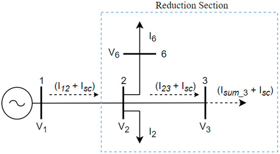
Figure 3.
Single line diagram of reduction section 1 in fault condition.
Basically, it is assumed that there is a particular condition in the system voltage profile for each fault situation occurring in a specific node, which means that the meters installed along the feeder will measure different voltage values when a bus is under fault.
Considering that a fault occurs in a time window of state estimation in normal operation, the fault location algorithm is started using data from supervisory system, specifically measures of voltage and current, when a fault is identified by protection relays. Sequentially, short circuits will be simulated in each node of the system, considering in all cases the fault current as the variation between the fault and pre-fault currents obtained by the substation meter. For each situation, NB-1 sets of estimated voltages will be generated for the other system nodes, including those with meters, where NB refers to the number of buses of the system. Loads have variations of current initially equals to zero, but larger variations can occur if were observed changes of estimated voltage magnitude at their respective installation points. In this way, during the iterative process of system sweeping and re-estimating, the algorithm will update the value of currents passing at each reduction section under analysis when recalculating the current contribution of the loads and the value of fault current in the supposed faulted node, until the convergence be reached. The modeling of loads in the fault location process will be described in Section 5.3.1.
The most probable node under fault will be the one that has the smallest error between the set of measured values and the set of estimated values, calculated by Equation (44).
In Equation (44), refers to the index of a meter that belongs to the set of k distribution meters, disregarding the one located at substation, and α-index is used to indicate the analyzed phase, since the proposed algorithm executes the estimation process per phase.
The developed fault location algorithm may be described in the following steps:
- Step 1: Obtain the voltage and current phasors at the substation (fault and pre-fault).
- Step 2: Model load impedances based on the last pre-fault state estimation report.
- Step 3: Select a system node and assume it as the supposed faulted node.
- Step 4: Perform the state estimation process and obtain the estimated voltage profile.
- Step 5: Compare the estimated and measured voltages and calculate the error by Equation (44).
- Step 6: If there is still a node to analyze
- Return to step 3
- Or
- Identify the bus with the lowest error
- Step 7: Indicate the fault location.
The use of reduction sections in the proposed fault location method also contributes to better algorithm processing. In fault location methods that use traditional state estimators, as shown in [28], the vectors and matrices used in the estimation have dimensions defined by the number of system nodes, usually numerous, which makes the fault location process slower.
5.3.1. Load Modeling in Fault Condition
Fault locating methods applied to distribution systems adopt different ways to model the loads, in order to calculate their respective current contributions during the fault. For example, Gord et al. [9] proposes a fault location algorithm based on Zbus matrix, in which the loads are modeled as constant impedances and are obtained from Equation (45). In fact, this approach solves the problem in some situations, but it does not represent the ideal modeling of a distribution network, since there are particularities in this type of network that were disregarded by authors as imbalance, the type of connected loads, variation in current profiles in light and heavy loading periods, besides the possibility of high and low impedance faults.
In Equation (45), and are nominal voltage and power, respectively, considering a power factor of 0.92 for all estimated loads.
Pereira et al. [29] presents a treatment to calculate the current contribution of loads in a more dynamic way, where the loads are modeled as constant powers and the transformers power rating are determined using a load flow routine proposed by Cheng and Shirmohammadi [30]. In this case, the values measured at substation are used as a reference to determine all system loads, however, does not use pseudo-measurements by state estimation or meter data along the feeder to decrease the degree of uncertainty of these loads.
As proposed work is a real-time application, the state estimator calculates the values of voltages and currents of all nodes at each time window, according to scheme shown in Figure 4, including the instant of occurrence of a fault.
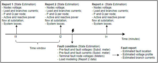
Figure 4.
System supervision by the proposed linearized state estimator.
After estimating voltages and currents, an impedance per phase can be assigned for each node to represent its load. By this approach, unbalance characteristic of the system is considered during the modeling of loads, because for the same node, each phase has different loads and utilization factors, providing different voltage and current values, and consequently different impedances per phase. Thus, the load modeling defined by linear state estimator based on currents summation considers that for the phase α of a bus the estimated load is a ratio between estimated voltage, , and estimated current, , according to Equation (46).
6. Results
The simulations were carried out in a real 58-node distribution system with a nominal voltage of 13.8 kV, located in northeastern Brazil. Figure 5 shows the system topology. The simulations of the state estimator were performed in MATLAB™, with input data from measurements of the supervisory system (normal operation condition) and obtained from the network modeled in ATP software [31], which made it possible to emulate measurements from short circuit simulations.
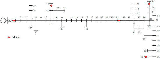
Figure 5.
Real urban distribution system (58 nodes).
Regarding meters allocation, the system was tested with 5 measuring devices: 1 measurement set located at substation, 1 recloser (with a measurement module) located at node 21 and three voltage meters located at buses 36, 42 and 55.
6.1. Results of State Estimator in Normal Operation
Results obtained using the linear current summation state estimator are presented in Table 1. It shows a comparison between measured and estimated values of currents and power flows at the substation, as well the estimated losses. Table 2 contains corresponding results obtained by use of the same algorithm but adding an iterative re-estimation process. The recloser installed at node 21 is equipped with a measurement module which is able to measure power flows, current and voltage magnitudes and transmit these data to an operation and control center. From these measurements both the utilization and load imbalance factors are calculated for each time window, and posteriorly the pseudo-measurements are determined to be used in the state estimation process. In order to demonstrate the robustness of the proposed estimator even using a small number of meters, in normal operating condition, only measures from substation and from equipment of node 21 were used in the state estimation algorithm to obtain the results of Table 1 and Table 2. The non-use of voltage measurements at terminal nodes does not significantly impact the obtained results, considering that the algorithm does not need this data to calculate the factors that determine the magnitudes of the pseudo-measured currents. In addition, from a computational and methodological point of view, the replacement of pseudo-measured voltages into measured values at nodes 36, 42, and 55, in the forward sweep step, are not very expressive, because there are no ramifications at primary network downstream of these points, then the use of these meters would influence only its variances. The nominal voltage of network is 13.8 kV, but the middle-voltage bus-bar of the substation has the voltage controlled at 14.1 kV.

Table 1.
Result for estimated system losses and comparison between measured and estimated data at the substation.
Table 2.
Result for estimated system losses and comparison between measured, estimated and re-estimated data at substation.
The convergence of the system state re-estimation process, using a tolerance of 1 × 10⁻³ p.u., occurs in three iterations, demonstrating that both estimation and load adjustment algorithms provides values close to measured data. A joint analysis of Table 1 and Table 2 shows that there is no significant variation when implementing a state re-estimation process compared to the methodology initially proposed. However, the re-estimation process assures that the minimum of the objective function has been reached.
6.2. Fault Location Results Based on State Estimation
In this section, the influence of four parameters on the proposed algorithm will be analyzed: (i) the location of the fault in the feeder, (ii) the fault resistance, (iii) the type of fault and (iv) the load level. The simulations were performed using the ATP and MATLAB™ software to implement the algorithms, and the distribution network shown in Figure 5. In ATP the system was modeled with loads defined as constant grounded-wye impedance, as shown in Figure 6. Thus, the voltage and current phasors of the substation and the magnitudes of the meters installed in the terminal nodes are obtained in ATP, and then exported to MATLAB™, where the fault location algorithm is processed. Contrary to the analysis in normal operation regime, in the fault condition it is essential to install voltage meters at some terminal nodes for the correct application of Equation (44), since the estimated values for these nodes will be compared with the measured values. A detailed analysis on observability and influence of the number of meters installed in the system is shown in Section 6.2.1.
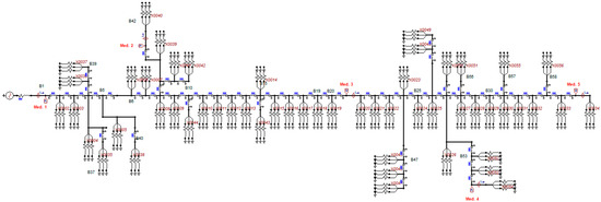
Figure 6.
Real urban distribution system (58 nodes) modeled in the alternative transient program (ATP) software.
6.2.1. Fault Location Analysis
In order to verify the influence of fault position in the analyzed distribution system, line-to-ground faults were simulated in all nodes, each one once a time, with a 10 Ω fault resistance. For each supposed bus under fault, sequentially, NB-1 nodal line-to-ground voltages were calculated, totaling at the end 3249 values per phase. Thus, the calculated voltages at measurements points will be compared to measured voltages at measurements points, for each fault condition, and the faulted bus will be the one with the smallest error indicated by Equation (44). It was noticed that in lateral branches without measurement in their respective terminal nodes, i.e., outside of the observable region, the estimator locates the main trunk bus of the feeder where the branching occurred. From this observation, three cases were analyzed: in the first (Case 1), the fault location errors were calculated considering the distance between the bus located outside of the observable region and the bus where the branch started, while in the second case (Case 2) only the bus contained in the observable region was considered. Thus, if there is a fault in a bus located in a branch without meters, the closest node from which this branch started should be located, and it must be contained in the system observable region. For Cases 1 and 2, meters were allocated to nodes 36, 42, and 55, in addition to the substation meter and the switch located at bus 21. Case 3 analyzed the influence of installing additional meters at nodes 37, 40, 44, 49, 51, and 56. From the analysis of Figure 7, it is possible to verify that the developed fault location algorithm has good precision for most of the analyzed situations. Taking into account that the distance between successive support structures (spans) in a medium voltage line is about 40 m, the maximal error resulting for this case corresponds to 7.6 spans. That is, in a practical situation the maintenance team would have visual access of the fault location covering only a small portion of the feeder.
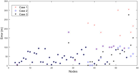
Figure 7.
Location error for different fault positions.
The largest location errors were observed in the nodes that do not contain measurement, while the smallest errors were found in the nodes closest to meters. The reduction of errors (ε) at buses located on lateral branches without measurement can be obtained by installing meters on terminal nodes, as observed in Case 3.
As example, a phase-to-ground short circuit occurring at bus 20, phase A, with a fault resistance of 10 Ω was tested, in order to details the algorithm operation. The allocation of meters used is the same as in Case 1. According Section 5.2, there is an estimated voltage profile for each fault situation. Thus, in Figure 8, for a better understanding, line-to-ground faults were simulated on nine different nodes (5, 10, 15, 19, 20, 21, 25, 30, and 35). Note that the average variation between the measured voltages and the estimated voltages, for situation where bus 20 is the supposed bus under fault, is the smallest among those analyzed, then, the locator defines that bus 20 is the closest bus to the point under fault through the index calculated by Equation (44).
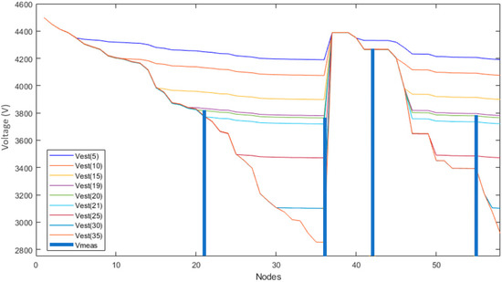
Figure 8.
Line-to-ground voltage profiles (phase A) considering faults applied to different nodes.
6.2.2. Influence of Fault Resistance
One of the main factors that influence the performance of impedance-based fault location methodologies is the fault resistance [30]. In order to analyze the influence of fault resistance, line-to-ground faults were simulated to all nodes of the system, with fault resistances (Rf) of 10, 20, 40, 80, and 100 Ω. The results obtained are shown in Table 3. Note that in the worst case, more than 80% of the faults were located with errors smaller than 200 m. The biggest errors came from faults with high impedances. The reasons for these larger errors can be explained by absence of meters on terminal branching nodes located in the most distant regions of the feeder root, such as the branching of buses 47, 48, 49, 51, and 58. These errors can be reduced with the installation of new meters in terminal nodes of these branches. Furthermore, it was noted that when the fault resistance increases and the short-circuit current decreases, the voltage variations between the nodes tend to decrease (as observed in curves of Rf = 80 Ω and Rf = 100 Ω of Figure 9), as expected, due to the fact that higher ground resistances tend to cause phase-to-ground faults in a node to behave as low-power single-phase loads, consequently causing small voltage drops. As voltages in the nodes are higher in faults with high impedance, there is a greater contribution of the load currents in these situations, especially in regions more distant from the trunk nodes of the feeder, due to accumulated impedance of cables. Even in these extreme situations, the proposed algorithm proved to be effective in its purpose.
Table 3.
Number of faults by class of error for different fault resistances.
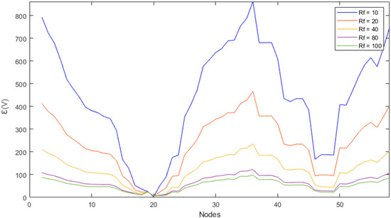
Figure 9.
Voltage profiles considering different faults resistance.
To exemplify the second case, bus 20 will be considered under fault condition and the error will be analyzed in terms of Rf variation.
6.2.3. Fault Type
Figure 10 shows the results of the method considering three different types of faults: line-to-ground (LG), line-to-line (LL), and three-phase (LLL). The fault resistance is 10 Ω for line-to-ground faults. All branches of the feeder were considered, not only those belonging to observable region (between two meters).
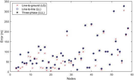
Figure 10.
Fault location error for different types of faults.
By analyzing Figure 10, only 71% of all simulated faults presented errors smaller than 100 m. Moreover, a little influence of fault type in the developed location method has resulted. The biggest errors were obtained in nodes located in lateral branches and in those more distant from the meters. As seen in Section 6.2.1, errors could be considered minor if only the observable region was considered. However, for a large distribution system, it is more interesting to provide the installation of meters on terminal nodes to make the localization process more accurate.
6.2.4. Influence of Load Level
In order to verify the performance of proposed fault location due to system load levels and load modeling on the proposed fault location process, simulations were performed considering the periods of light and heavy load of the distribution system shown in Figure 5. The currents used to calculate the utilization factor were obtained from the substation meter. The utilization factors, per phase, for cited periods are shown in Table 4.
Table 4.
Utilization factor in light and heavy load periods.
Four cases were analyzed: light load and heavy load simulations, considering the load modeling proposed in this work and comparing it with the load model that considers a fixed impedance value, according to Equation (37). Line-to-ground faults with Rf = 10 Ω were simulated in all cases. It is possible to observe in Figure 11 that the dynamic load modeling based on linear state estimation provides more accurate results when compared to the method that uses a fixed impedance value for the loads, regardless of the system load. The dotted lines between the nodes in Figure 11 were used only to connect their values graphically, to assist in the interpretation of the results, since there is not necessarily a physical connection between the nodes in the same numerical sequence in which they are shown on the x axis.
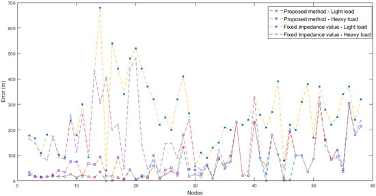
Figure 11.
Fault location error for different types of faults.
By simulations, it was possible to verify that the incorrect determination of estimated load impedances causes an erroneous variation of the estimated fault currents for each bus, modifying the estimated nodes voltages at the moment of the short circuit and, consequently, generating higher values of fault location error.
7. Discussion
The main purpose of this article is to develop a linear state estimator based on the current summation load flow method for real time application and for fault location in energy distribution systems. The proposed work can be applied to unbalanced three-phase networks, considering that the formulation is done by phase. The first stage of the research aimed to apply the estimation methodology in the network supervision under normal operation, allowing the operator to monitor system parameters such as bus voltage, branch currents, and losses in the network, even with a reduced number of meters allocated along the feeder. Besides monitoring, these parameters are fundamental in parameterizing equipment for system protection and serve as a reference for future updates of the feeder infrastructure. Subsequently, a state re-estimation process was tested, where a small influence was observed on the results, when compared with the corresponding ones obtained from estimator without the re-estimation process. This means that the pseudo-measurements and the values calculated in the estimation process have good proximity to the measured values.
The main advantages of first stage, corresponding to the proposed state estimation are: (i) the use of a reduced number of meters to estimate the system state; (ii) linearization of equations to reduce the computational effort required at each time window of estimation; (iii) use of pseudo-measurements to compensate the reduced number of meters; and (iv) dynamic modeling of loads for network supervision in real time.
A second objective was to propose the application of the estimator in the fault location process. In this case, the algorithm proved to be promising in its function, locating defects even with high fault resistances. The method performs the integration between the state estimator in the situation of normal operation regime and the fault locator, which provides, through dynamic modeling of loads, and the possibility of analyzing their contributions to the short circuit. Since the estimator provides the voltage phasors at the substation, as well as the contributions of the load currents to the short circuit, a preliminary step of fault classification becomes unnecessary. The fault locator depends exclusively on the information resulting from the state estimator.
The obtained results show that faults occurring closer to meters have good precision in the localization process, while by most distant faults from meter it tends to become less accurate, since uncertainties contained in the electrical quantities involved in these cases are higher, as would be expected according to theory of errors propagation. Only 4 m allocated to the feeder were used, in addition to the substation measurement, which corresponds to approximately 7% of measuring nodes. No meter allocation technique had to be used, since the algorithm provided good results for analyzed cases. The influence of load level and the way the load impedances are calculated were also investigated in the fault location process. Considering the proposed dynamic load modeling, it was possible to observe a minimal variation of fault location errors comparing the periods of light load and heavy, while the use of loads represented by impedances with fixed values was not recommended for proposed fault location algorithm.
The average execution time for an iteration of a system reduction section is 0.003 s, this value can serve as reference for estimating the execution time for feeders with a higher number of nodes. Table 5 shows the execution time, per unit (base 0.003 s), of the linear state estimator under normal and fault conditions. The computer used was an Asus notebook with Intel® Core ™ I5 3210M 2.5GHz, Memory (RAM) 6 GB and 64-bit OS. The developed algorithms were written and simulated in the MATLAB™ software. It was verified, based on the measured execution times, that the proposed linear state estimator for distribution networks has potential for application in real time systems supervision.
Table 5.
Execution times for a real urban distribution system (Figure 5).
An apparent disadvantage of the proposed fault location method is that in lateral branches without measurement, the algorithm indicates the faulted node as being the one located in the main trunk of the feeder, where the branch begins. Thus, it returns the same error ε for these nodes, which means that not the whole system is observable. Although these cases comprise a small portion of the system, the adoption of an optimized meter allocation strategy can contribute to solve the problem.
8. Conclusions
Power distribution systems are commonly susceptible to failures that can provide interruption of electricity supply. Its complex topology associated with a reduced number of meters makes the process of fault location difficult and contributes to increase indices that measure the time of interruptions. This work proposed a new linear state estimator based on the current summation for monitoring the system in real time, applied for normal operating conditions and in cases of faults. The deficit of measured data along the feeder is compensated by use of pseudo-measurements. At each time window of the state estimator, the algorithm automatically updates both the utilization, and the load imbalance factors, making it possible to estimate the currents and voltages at each system node, the power flow, and the system losses. The linearization of state estimator through the use of load flow method based on currents summation proved to be advantageous due to the simplification of equations, which results in a reduced level of computational effort and total execution time of developed algorithm, making it apposite for real-time applications.
Another novelty of this work was the development of a specific state estimator for distribution networks that can also be applied to fault location using data estimated in real time. Related articles that analyze fault location using state estimation methods generally use techniques used in power transmission systems and simplifications and considerations that do not consider the specificities of distribution networks. In the proposed method, fault location process is initiated based on the last time window of estimator, making possible analyze more accurately the relationship between the magnitude of the fault current and contribution of load currents during the short circuit. The performance of the method proved to be promising by short circuit simulations with low and high impedance faults and in periods of light and heavy load, proving the effectiveness in estimating loads and voltage profile by the linear state estimator.
State estimators for distribution networks from related research are successfully used in feeders located in northeastern Brazil. However, modifications to the system that provide a three-phase analysis and fault location have not yet been implemented. This is a next step in this project. Studies about optimal meter placement (OPM) and application of the proposed estimator in distribution networks with distributed generation are future objectives of this research.
Author Contributions
Conceptualization, E.R. and M.M.J.; methodology, E.R., M.P.F., and M.M.J.; software, E.R., M.P.F., M.A., and M.M.J.; formal analysis, E.R., M.P.F., and M.M.J.; investigation, E.R., M.P.F., and M.M.J.; data curation, E.R.; writing—original draft preparation, E.R.; writing—review and editing, M.P.F., M.A., M.C., and M.M.J.; visualization, E.R. and M.P.F.; supervision, M.M.J.; project administration, M.M.J.; funding acquisition, E.R. All authors have read and agreed to the published version of the manuscript.
Funding
This study was financed in part by the Coordenação de Aperfeiçoamento de Pessoal de Nível Superior–Brasil (CAPES)–Finance Code 001.
Conflicts of Interest
The authors declare no conflict of interest.
Nomenclature
| z | Vector of measurements |
| x | Vector of state variables |
| h(x) | Vector of functions |
| e | Error vector of the measurements and pseudo-measurements |
| σ2 | Variance |
| Rz | Covariance matrix |
| J(x) | Objective function of estate estimation |
| G(x) | Gain matrix |
| g(x) | Gradient of J(x) |
| fu | Utilization factor |
| fp | Power factor |
| Fimb | Factor of load imbalance |
| Dm | Maximum demand |
| Imea | Measured phase current |
| IT | Rated current of a distribution transformer |
| IGA | Rated current of a transformer (Group A—Private client equipment) |
| ST | Total power required by a load |
| SN | Rated power of a distribution transformer |
| Sph | Power required by a load (per phase) |
| Jlm | Branch current between l and m nodes |
| Zlm | Branch impedance between l and m nodes |
| Ploss | Active loss |
| Qloss | Reactive power balance |
| ε | Estimation error |
References
- Singh, R.; Pal, B.C.; Jabr, R.A. Distribution system state estimation through Gaussian mixture model of the load as pseudo-measurement. IET Gener. Transm. Distrib. 2010, 4, 50–59. [Google Scholar] [CrossRef]
- Manitsas, E.; Singh, R.; Pal, B.C.; Strbac, G. Distribution system state estimation using an artificial neural network approach for pseudo measurement modeling. IEEE Trans. Power Syst. 2012, 27, 1888–1896. [Google Scholar] [CrossRef]
- Schweppe, F.C.; Debs, A.S. Power System Static-State Estimation—Part I. Available online: https://ieeexplore.ieee.org/document/4074022 (accessed on 14 November 2019).
- Oner, A.; GOL, M. Fault location based on state estimation in PMU observable systems. IEEE Power Energy Soc. Innov. Smart Grid Technol. Conf. 2016. [Google Scholar] [CrossRef]
- Personal, E.; García, A.; Parejo, A.; Larios, D.F.; Biscarri, F.; León, C. A Comparison of Impedance-Based Fault Location Methods for Power Underground Distribution Systems. Energies 2016, 9, 1022. [Google Scholar] [CrossRef]
- Sun, K.; Chen, Q.; Zhao, P. Automatic Faulted Feeder Section Location and Isolation Method for Power Distribution Systems Considering the Change of Topology. Energies 2017, 10, 1081. [Google Scholar] [CrossRef]
- Le, D.P.; Bui, D.M.; Ngo, C.C.; Le, A.M.T. FLISR Approach for Smart Distribution Networks Using E-Terra Software—A Case Study. Energies 2018, 11, 3333. [Google Scholar] [CrossRef]
- Li, J. Augmented State Estimation Method for Fault Location Based on On-line Parameter Identification of PMU Measurement Data. In Proceedings of the 2018 IEEE 2nd International Electrical and Energy Conference (Cieec), Beijing, China, 1–5 November 2018. [Google Scholar]
- Gord, E.; Dashti, R.; Najafi, M.; Shaker, H.R. Real Fault Section Estimation in Electrical Distribution Networks Based on the Fault Frequency Component Analysis. Energies 2019, 12, 1145. [Google Scholar] [CrossRef]
- Cavalcante, A.H.; de Almeida, M.C. Fault location approach for distribution systems based on modern monitoring infrastructure. IET Gener. Transm. Distrib. 2018, 12, 94–103. [Google Scholar] [CrossRef]
- Dashti, R.; Sadeh, J. Applying Dynamic Load Estimation and Distributed-parameter Line Model to Enhance the Accuracy of Impedance-based Fault-location Methods for Power Distribution Networks. Electr. Power Compon. Syst. 2013, 41, 1334–1362. [Google Scholar] [CrossRef]
- Vieira, F.L.; Santos, P.H.M.; Carvalho Filho, J.M.; Leborgne, R.C.; Leite, M.P. A Voltage-Based Approach for Series High Impedance Fault Detection and Location in Distribution Systems Using Smart Meters. Energies 2019, 12, 3022. [Google Scholar] [CrossRef]
- Li, H.; Mokhar, A.S.; Jenkins, N. Automated Fault Location on Distribution Network Using Voltage Sags Measurements. Available online: https://www.researchgate.net/publication/224122767_Automatic_fault_location_on_distribution_network_using_voltage_sags_measurements (accessed on 13 January 2020).
- Almeida, M.A.D.; Medeiros, M.F., Jr.; Silveira, D.B.F. Estimating Loads in Distribution Feeders Using a State Estimator Algorithm with Additional Adjustment of Transformers Loading Factors. In Proceedings of the IEEE International Symposium on Circuits and Systems-ISCAS, Bangkok, Thailand, 25–28 May 2003. [Google Scholar]
- Crow, M.L. Computational Methods for Electric Power Systems; CRC Press: Boca Raton, FL, USA, 2010. [Google Scholar]
- Monticelli, A.J. State Estimation in Electric Power Systems; Kluwer Academic Publishers: Cambridge, MA, USA, 1999. [Google Scholar]
- Manitsas, E.; Singh, R.; Pal, B.; Strbac, G. Modelling of Pseudo-Measurements for Distribution System State Estimation. Available online: https://www.researchgate.net/publication/4360537_Modeling_of_pseudo-measurements_for_distribution_system_state_estimation (accessed on 13 January 2020).
- Medeiros, M.F.M., Jr.; Almeida, M.A.D.; Cruz, M.C.S.; Monteiro, R.V.F.; Oliveira, A.B. A three-phase algorithm for state estimation in power distribution feeders based on the power summation load flow method. Electr. Power Syst. Res. 2015, 123, 76–84. [Google Scholar] [CrossRef]
- Shirmohammadi, D.; Hong, H.W.; Semlyen, A. Compensation based power flow method for weakly meshed distribution and transmission networks. IEEE Trans. Power Syst. 1988, 3, 753–762. [Google Scholar] [CrossRef]
- Thukaram, D.; Banda, H.M.W.; Jeroni, J. A robust three phase power flow algorithm for radial distribution systems. Electr. Power Syst. Res. 1999, 3, 227–236. [Google Scholar] [CrossRef]
- Zhu, Y.; Tomsovic, K. Adaptive power flow method for distribution systems. IEEE Transl. Power Deliv. 2002, 17, 822–827. [Google Scholar]
- Ciric, R.M.; Feltrin, A.P.; Rocha, L.F. Power Flow in four-wire distribution networks—general approach. IEEE Trans. Power Syst. 2003, 18, 1283–1290. [Google Scholar] [CrossRef]
- Kersting, W.H. Distribution System Modeling and Analysis, 4th ed.; CRC Press: New York, NY, USA, 2017. [Google Scholar]
- ISO. Guide to the Expression of Uncertainty in Measurement; International Organization for Standardization: Geneva, Switzerland, 1995. [Google Scholar]
- Vuolo, J.H. Fundaments of Error Theory; Ed. Edgar Blücher: São Paulo –SP, Brazil, 1992; 225p. [Google Scholar]
- LEE, S.-J.; Choi, M.-S.; Kang, S.-H.; Jin, B.-G.; Lee, D.-S.; Ahn, B.-S.; Yoon, N.-S.; Kim, H.-Y.; Wee, S.-B. An Intelligent and Efficient Fault Location and Diagnosis Scheme for Radial Distribution Systems. IEEE Trans. Power Deliv. 2004, 19, 524–532. [Google Scholar] [CrossRef]
- Trindade, F.C.L.; Freitas, W.; Vieira, J.C.M. Fault Location in Distribution Systems Based on Smart Feeder Meters. IEEE Trans. Power Deliv. 2014, 29, 251–260. [Google Scholar] [CrossRef]
- Cavalcante, A.H. Fault Location Approaches for Modern Power Distribution Systems. Ph.D Thesis, University of Campinas, Campinas, São Paulo, Brazil, 2016. [Google Scholar]
- Pereira, R.A.F.; Silva, L.G.W.; Kezunovic, M.; Mantovani, J.R.S. Improved Fault Location on Distribution Feeders Based on Matching During-Fault Voltage Sags. IEEE Trans. Power Deliv. 2009, 24, 852–862. [Google Scholar] [CrossRef]
- Cheng, C.S.; Shirmohammadi, D. A three-phase power flow method for real-time distribution system analysis. IEEE Trans. Power Syst. 1995, 10, 671–679. [Google Scholar] [CrossRef]
- Leuven EMTP Center: Alternative Transients Program—Rule Book. 1987. Available online: https://www.scirp.org/(S(lz5mqp453edsnp55rrgjct55))/reference/ReferencesPapers.aspx?ReferenceID=67302 (accessed on 27 January 2020).
© 2020 by the authors. Licensee MDPI, Basel, Switzerland. This article is an open access article distributed under the terms and conditions of the Creative Commons Attribution (CC BY) license (http://creativecommons.org/licenses/by/4.0/).